4.8Measures of risk in a financial market

In this section, we will consider risk measures which arise in the financial market model of Section 1.1. In this model, d + 1 assets are priced at times t = 0 and t = 1. Prices at time 1 are modeled as nonnegative random variables S0, S1, . . . , Sd on some probability space (Ω,F, P), with S0 ≡ 1 + r. Prices at time 0 are given by a vector = (1, π), with π = (π1, . . . , πd). The discounted net gain of a trading strategy = (ξ0, ξ) is given by ξ · Y, where the random vector Y = (Y1, . . . , Yd) is defined by

As in the previous two sections, risk measures will be defined on the space L∞ = L∞(Ω,F, P). A financial position X can be viewed as riskless if X ≥ 0 or, more generally, if X can be hedged without additional costs, i.e., if there exists a trading strategy = (ξ0, ξ) such that · = 0 and

Thus, we define the following set of acceptable positions in L∞:

Proposition 4.99. Suppose that inf{m ∈ ℝ | m ∈ A0} > −∞. Then ρ0 := ρA0 is a coherent risk measure. Moreover, ρ0 is sensitive in the sense of Definition 4.42 if and only if the market model is arbitrage-free. In this case, ρ0 is continuous from above and can be represented in terms of the set P of equivalent risk-neutral measures:

Proof. The fact that ρ0 is a coherent risk measure follows from Proposition 4.7. If the model is arbitrage-free, then Theorem 1.32 yields the representation (4.66), and it follows that ρ0 is sensitive and continuous from above.

Conversely, suppose that ρ0 is sensitive, but the market model admits an arbitrage opportunity. Then there are ξ ∈ ℝd and ε > 0 such that 0 ≤ ξ · Y P-a.s. and A := {ξ · Y ≥ ε} satisfies P[ A ] > 0. It follows that ξ · Y − εA ≥ 0, i.e., −εA is acceptable. Thus, the positive homogeneity of ρ0, which follows from the fact that A0 is a cone, implies that ρ0(−λA )≤ 0 for any λ > 0. On the other hand, Theorem 4.43 implies that ρ0(−λA) > ρ0(0) = 0 for some (and hence all) λ > 0. This is the desired contradiction.

There are several reasons why it may make sense to allow in (4.65) only strategies ξ that belong to a proper subset S of the class ℝd of all strategies. For instance, if the resources available to an investor are limited, only those strategies should be considered for which the initial investment in risky assets is below a certain amount.

Such a restriction corresponds to an upper bound on ξ · π. There may be other constraints. For instance, short sales constraints are lower bounds on the number of shares in the portfolio. In view of market illiquidity, the investor may also wish to avoid holding too many shares of one single asset, since the market capacity may not suffice to resell the shares. Such constraints will be taken into account by assuming throughout the remainder of this section that S has the following properties:

–0∈ S.

–S is convex.

–Each ξ ∈ S is admissible in the sense that ξ · Y is P-a.s. bounded from below.

Under these conditions, the set

is nonempty, convex, and contains all X ∈ X which dominate some Z ∈ A S . Moreover, we will assume from now on that

Proposition 4.7 then guarantees that the induced risk measure

is a convex risk measure on L∞. Note that (4.68) holds, in particular, if S does not contain arbitrage opportunities in the sense that ξ · Y ≥ 0 P-a.s. for ξ ∈ S implies P[ ξ · Y = 0] = 1.

Remark 4.100. Admissibility of portfolios is a serious restriction; in particular, it prevents unhedged short sales of any unbounded asset. Note, however, that it is consistent with our notion of acceptability for bounded claims in (4.67), since X +ξ ·Y ≥ 0 implies

◊

Two questions arise: When is ρS continuous from above, and thus admits a representation (4.34) in terms of probability measures? And, if such a representation exists, how can we identify the minimal penalty function on M1(P)? In the case S = ℝd, both questions were addressed in Proposition 4.99. For general S, only the second question has a straightforward answer, which will be given in Proposition 4.102. As can be seen from the proof of Proposition 4.99, an analysis of the first question requires an extension of the arbitrage theory in Chapter 1 for the case of portfolio constraints. Such a theory will be developed in Chapter 9 in a more general dynamic setting, and we will address both questions for the corresponding risk measures in Corollary 9.32. This result implies the following theorem for the simple one-period model of the present section:

Theorem 4.101. In addition to the above assumptions, suppose that the market model is nonredundant in the sense of Definition 1.15 and thatS is a closed subset ofℝd such that the cone {λξ | ξ ∈ S , λ ≥ 0} is closed. Then ρS is sensitive if and only if S contains no arbitrage opportunities. In this case, ρS is continuous from above and admits the representation

In the following proposition, we will explain the specific form of the penalty function in (4.69). This result will not require the additional assumptions of Theorem 4.101.

Proposition 4.102. For Q ∈ M1(P), the minimal penalty function is given by

In particular, ρS can be represented as in (4.69) if ρS is continuous from above.

Proof. Fix Q ∈ M1(P). Clearly, the expectation EQ[ ξ · Y ] is well defined for each ξ ∈ S by admissibility. If X ∈ A S , there exists η ∈ S such that −X ≤ η · Y P-almost surely. Thus,

for any Q ∈ M1(P). Hence, the definition of the minimal penalty function yields

To prove the converse inequality, take ξ ∈ S. Note that Xk := −((ξ · Y) ∧ k) is bounded since ξ is admissible. Moreover,

so that Hence,

and so by monotone convergence.

Exercise 4.8.1. Show that the identity

in Proposition 4.102 remains true even for Q ∈ M1,f (P) if we assume in addition that Y is P-a.s. bounded. We thus obtain the representation

without assuming continuity from above.

◊

Remark 4.103. Suppose that S is a cone. Then the acceptance set A S is also a cone, and ρS is a coherent measure of risk. If ρS is continuous from above, then Corollary 4.37 yields the representation

in terms of the nonempty setIt follows from Proposition 4.102 that for Q ∈ M1(P)

If ρS is sensitive, then the set S cannot contain any arbitrage opportunities, and QS contains the set P of all equivalent martingale measures whenever such measures exist. More precisely, QS can be described as the set of absolutely continuous super-martingale measures with respect to S; this will be discussed in more detail in the dynamical setting of Chapter 9.

Let us now relax the condition of acceptability in (4.67). We no longer insist that the final outcome of an acceptable position, suitably hedged, should always be nonnegative. Instead, we only require that the hedged position is acceptable in terms of a given convex risk measure ρA with acceptance set A . Thus, we define

Clearly, A ⊂ A¯ and hence

From now on, we assume that

which implies our assumption (4.68) for A S .

Proposition 4.104. The minimal penalty function αmin for ρ is given by

where is the minimal penalty function for ρS and αmin is the minimal penalty function for ρA .

Proof. We claim that

If ρ(X) < 0, then X ∈ A¯. Hence, there exists A ∈ A and ξ ∈ S such that X + ξ · Y ≥ A. Therefore XS := X − A ∈ A S , and we obtain the first inclusion in (4.74). To prove the second inclusion, take XS ∈ A S . Then there exists ξ ∈ S such that XS + ξ · Y ≥ 0. Hence, for any A ∈ A , we get XS + A + ξ · Y ≥ A ∈ A , i.e., X := XS + A ∈ A¯. This establishes the second inclusion in (4.74).

Now let Q ∈ M1,f be given. In view of (4.74), we have

But the left- and rightmost terms in the preceding chain of inequalities are equal, and so we get that

Remark 4.105. It can happen that the sum of two penalty functions as on the right-hand side of (4.73) is infinite for every Q ∈ M1,f (P). In this case, the condition (4.72) will be violated and the risk measure ρ does not exist. Consider, for example, the

situation of a complete market model without trading constraints. Then ρS (X) = E∗[ −X ], where P∗ is the unique equivalent risk-neutral measure. That is,

For ρA we take AV@Rλ. Then is infinite for Q ≠ P∗, and is finite (and in fact zero) if and only if

But the latter condition is violated as soon as P∗ ≠ P and λ is close enough to 1.

◊

Exercise 4.8.2. Suppose that condition (4.72) is satisfied. Show that the risk measure ρ can also be obtained as

and as

◊

The preceding exercise shows that ρ is a special case of an inf-convolution, which we now define in a general context.

Definition 4.106. For two convex risk measures ρ1 and ρ2 on L∞,

is called the inf-convolution of ρ1 and ρ2.

◊

Exercise 4.8.3. Let ρ1 and ρ2 be two convex risk measures on L∞ and assume that

(a) Show that

(b) Show that is a convex risk measure on L∞.

(c) Show that the minimal penalty function αmin of ρ is equal to the sum of the respective minimal penalty functions and of ρ1 and ρ2:

(d) Show that ρ is continuous from below as soon as ρ1 is continuous from below.

◊

For the rest of this section, we consider the following case study, which is based on [47]. Let us fix a finite class

of equivalent probability measures Qi ≈ P such that |Y| ∈ L1(Qi); as in [47], we call the measures in Q0 valuation measures. Define the sets

and

Note that

since X = 0 P-a.s. as soon as X ≥ 0 P-a.s. and EQi [ X ] = 0, due to the equivalence Qi ≈ P.

As the initial acceptance set, we take the convex cone

The corresponding set A¯ of positions which become acceptable if combined with a suitable hedge is defined as in (4.71):

Let us now introduce the following stronger version of the no-arbitrage condition where

In other words, there is no portfolio ξ ∈ ℝd such that the result satisfies the valuation inequalities in (4.75) and is strictly favorable in the sense that at least one of the inequalities is strict.

Note that (4.78) implies the absence of arbitrage opportunities:

where we have used (4.76) and Thus, (4.78) implies, in particular, the existence of an equivalent martingale measure, i.e.,P ≠ ∅. The following proposition may be viewed as an extension of the “fundamental theorem of asset pricing”. Let us denote by

the class of all “representative” models for the class Q0, i.e., all mixtures such that each Q ∈ Q0 appears with a positive weight.

Proposition 4.107. The following two properties are equivalent:

(a)

(b)

Proof. (b)⇒(a): For V ∈ K ∩ B and R ∈ R, we have ER[ V ]≥ 0. If we can choose

R ∈ P ∩ R then we get ER[ V ] = 0, hence V ∈ B0.

(a)⇒(b): Consider the convex set

we have to show that C contains the origin. If this is not the case then there exists ξ ∈ ℝd such that

and

see Proposition A.5. Define V := ξ · Y ∈ K . Condition (4.79) implies

hence V ∈ K ∩B. Let R∗ ∈ R be such that x∗ = ER∗ [ Y ]. Then V satisfies ER∗ [ V ] > 0, hence V ∈ / K ∩ B0, in contradiction to our assumption (a).

We can now state a representation theorem for the coherent risk measure ρ corresponding to the convex cone A¯. It is a special case of Theorem 4.110 which will be proved below.

Theorem 4.108. Under assumption (4.78), the coherent risk measure ρ := ρA¯ corresponding to the acceptance set A¯ is given by

Let us now introduce a second finite set Q1 ⊂ M1(P) of probability measures Q P with |Y| ∈ L1(Q); as in [47], we call them stress test measures. In addition to the valuation inequalities in (4.75), we require that an admissible position passes a stress test specified by a “floor”

Thus, the convex cone A in (4.77) is reduced to the convex set

where

Let

denote the resulting acceptance set for positions combined with a suitable hedge.

Remark 4.109. The analogue

of our condition (4.78) looks weaker, but it is in fact equivalent to (4.78). Indeed, for X ∈ K ∩ B we can find ε > 0 such that X1 := εX satisfies the additional constraints

Since X1 ∈ K ∩ B ∩ B1, condition (4.80) implies X1 ∈ K ∩ B0, hence ∈ K ∩ B0, since K ∩ B0 is a cone.

◊

Let us now identify the convex risk measure ρ1 induced by the convex acceptance set A¯1. Define

as the convex hull of Q := Q0 ∪ Q1, and define

for with

Theorem 4.110. Under assumption (4.78), the convex risk measure ρ1 induced by the acceptance set A¯1 is given by

i.e., ρ1 is determined by the penalty function

Proof. Let ρ∗ denote the convex risk measure defined by the right-hand side of (4.81), and let A ∗ denote the corresponding acceptance set:

It is enough to show A ∗ = A¯1.

(a): In order to showA¯1 ⊂ A ∗, take X ∈ A¯1 and P∗ ∈ P∩R1. There exists ξ ∈ ℝd and A1 ∈ A1 such that X + ξ · Y ≥ A1. Thus,

due to P∗ ∈ R1. Since E∗[ ξ · Y ] = 0 due to P∗ ∈ P, we obtain E∗[ X ]≥ γ(P∗), hence X ∈ A ∗.

(b): In order to show A ∗ ⊂ A¯ 1, we take X ∈ A ∗ and assume that X ∈/ A¯1. This means that the vector x∗ = (x∗1, . . . , x∗N) with components

does not belong to the convex cone

where Q = Q0 ∪ Q1 = {Q1, . . . , QN} with N ≥ n. In part (c) of this proof we will show that C is closed. Thus, there exists λ ∈ ℝN such that

see Proposition A.5. Since we obtain λi ≥ 0 for i = 1, . . . , N, and we may assumesince λ ≠ 0. Define

Since C contains the linear space of vectors EQi [ V ]with V ∈ K , (4.82) i=1,...,N implies

hence R ∈ P. Moreover, the right-hand side of (4.82) must be zero, and the condition λ · x∗ < 0 translates into

contradicting our assumption X ∈ A ∗.

(c): It remains to show that C is closed. For ξ ∈ ℝd we define y(ξ) as the vector in ℝN with coordinates yi(ξ) = EQi [ ξ · Y ]. Any x ∈ C admits a representation

with and ξ ∈ N⊥, where

and

Take a sequence

with ξn ∈ N⊥ and such that xn converges to If lim infn |ξn| < ∞, then we may assume, passing to a subsequence if necessary, that ξn converges to ξ ∈ ℝd. In this case, zn must converge to some and we have x = y(ξ) + z ∈ C . Let us now show that the case limn |ξn| = ∞is in fact excluded. In that case, αn := (1+|ξn|)−1 converges to 0, and the vectors ζn := αnξn stay bounded. Thus, we may assume that ζn converges to ζ ∈ N ⊥. This implies

Since ζ ∈ N⊥ and |ζ | = limn |ζn| = 1, we obtain y(ζ) ≠ 0. Thus, the inequality

holds for all i and is strict for some i, in contradiction to our assumption (4.78).

4.9Utility-based shortfall risk and divergence risk measures

In this section, we will establish a connection between convex risk measures and the expected utility theory of Chapter 2.

Suppose that a risk-averse investor assesses the downside risk of a financial position X ∈ X by taking the expected utility E[ u(−X−) ] derived from the shortfall X −, or by considering the expected utility E[ u(X) ] of the position itself. If the focus is on the downside risk, then it is natural to change the sign and to replace u by the function (x) := −u(−x). Then is a strictly convex and increasing function, and the maximization of expected utility is equivalent to minimizing the expected loss E[ (−X) ] or the shortfall risk E[ (X−) ]. In order to unify the discussion of both cases, we do not insist on strict convexity. In particular, may vanish on (−∞, 0], and in this case the shortfall risk takes the form

Definition 4.111. A function : ℝ → ℝ is called a loss function if it is increasing and not identically constant.

◊

Let us return to the setting where we consider monetary risk measures defined on the class X of all bounded measurable functions on some given measurable space (Ω,F). Let us fix a probability measure P on (Ω,F). For a given loss function and an interior point x0 in the range of , we define the following acceptance set:

Alternatively, we can write

where u(x) = −(−x) and y0 = −x0. The acceptance set A satisfies (4.3) and (4.4). By part (a) of Proposition 4.7 it induces a monetary risk measure ρ given by

This risk measure satisfies (4.33) and hence can be regarded as a monetary risk measure on L∞. If is convex or u concave, ρ is a convex risk measure. It is normalized when x0 = (0).

Exercise 4.9.1. Let be a strictly increasing continuous loss function. Suppose that the risk measure ρ associated to via (4.85) satisfies

for any X, Y ∈ L∞. Show that is either linear or exponential.

Hint: Apply Proposition 2.46.

◊

For the rest of this section, we will only consider convex loss functions.

Definition 4.112. The convex risk measure in (4.85) is called utility-based shortfall risk measure.

◊

Proposition 4.113. The utility-based shortfall risk measure ρ is continuous from below. Moreover, the minimal penalty function αmin for ρ is concentrated on M1(P), and ρ can be represented in the form

Proof. We have to show that ρ is continuous from below. Note first that z = ρ(X) is the unique solution to the equation

Indeed, that z = ρ(X) solves (4.87) follows by dominated convergence, since the finite convex function is continuous. The solution is unique, since is strictly increasing on (−1(x0)− ε,∞) for some ε > 0.

Suppose now that (Xn) is a sequence in X which increases pointwise to some X ∈ X . Then ρ(Xn) decreases to some finite limit R. Using the continuity of and dominated convergence, it follows that

But each of the approximating expectations equals x0, and so R is a solution to (4.87). Hence R = ρ(X), and this proves continuity from below. Since ρ satisfies (4.33), the representation (4.86) follows from Theorem 4.22 and Lemma 4.32.

The following exercise should be compared to Exercise 4.4.1.

Exercise 4.9.2. Let λ ∈ (0, 1) be given.

(a) Show that the following conditions are equivalent for X ∈ L2 and ζ ∈ ℝ.

(i) The number ζ minimizes the function

(ii) We have

A number ζ satisfying the preceding two equivalent conditions is called an expectile for X at level λ.

(b) Now consider the loss function (x) = (1 − λ)x+ − λx−, which is convex for λ ≤ 1/2. Show that, in this case, the corresponding shortfall risk measure

is such that −ρ(X) is an expectile for X at level λ.

◊

Let us now compute the minimal penalty function αmin of a utility-based shortfall risk measure. We start by analyzing the following special case.

Example 4.114. For an exponential loss function (x) = eβx, the minimal penalty function can be described in terms of relative entropy, and the resulting risk measure coincides, up to an additive constant, with the entropic risk measure introduced in Example 4.34. In fact,

In this special case, the general formula (4.20) for αmin reduces to the variational formula for the relative entropy H (Q|P) of Q with respect to P:

see Lemma 3.29. Thus, the representation (4.86) of ρ is equivalent to the following dual variational identity:

In general, the minimal penalty function αmin on M1(P) can be expressed in terms of the Fenchel–Legendre transform or conjugate function ∗ of the convex function defined by

Theorem 4.115. For any convex loss function , the minimal penalty function in the representation (4.86) is given by

In particular,

To prepare the proof of Theorem 4.115, we summarize some properties of the functions and ∗ as stated in Appendix A.1. First note that ∗ is a proper convex function, i.e., it is convex and takes some finite value. We denote by its right-continuous derivative. Then, for x, z ∈ ℝ,

Lemma 4.116. Let (n) be a sequence of convex loss functions which decreases pointwise to the convex loss function . Then the corresponding conjugate functions increase pointwise to ∗.

Proof. It follows immediately from the definition of the Fenchel–Legendre transform that each is dominated by ∗, and that increases to some limit We have to prove that

The function is a lower semicontinuous convex function as the increasing limit of such functions. Moreover, is a proper convex function, since it is dominated by the proper convex function ∗. Consider the conjugate function of Clearly, since and since = by Proposition A.9. On the other hand, we have by a similar argument for each n. By taking n ↑ ∞, this shows which in turn gives

Lemma 4.117. The functions and ∗ have the following properties.

(a) ∗(0) = − infx∈R (x) and ∗(z) ≥ −(0) for all z.

(b) There exists some z1 ∈ [0,∞) such that

particular, ∗ is increasing on [z1,∞).

(c)

Proof. Part (a) is obvious.

(b): Let N := {z ∈ ℝ | ∗(z) = −(0)}. We show in a first step that N ≠ ∅. Note that convexity of implies that the set S of all z with zx ≤ (x) − (0) for all x ∈ ℝ is nonempty. For z ∈ S we clearly have ∗(z) ≤ −(0). On the other hand, ∗(z) ≥ −(0) by (a).

Now we take z1 := sup N. It is clear that z1 ≥ 0. If z > z1 and x < 0, then

where the last inequality follows from the lower semicontinuity of ∗. But ∗(z) > −(0), hence

(c): For z ≥ z1,

by (b). Hence

where xz := sup{x | (x) ≤ z}. Since is convex, increasing, and takes only finite values, we have xz → ∞as z ↑ ∞.

Proof of Theorem 4.115. Fix Q ∈ M1(P), and denote by φ := dQ/dP its density. First, we show that it suffices to prove the claim for x0 > (0). Otherwise we can find some a ∈ ℝ such that (−a) < x0, since x0 was assumed to be an interior point of (ℝ). Let (x) := (x − a), and

Then = {X − a | X ∈ A }, and hence

The convex loss function satisfies the requirement (0) < x0. So if the assertion is established in this case, we find that

here we have used the fact that the Fenchel–Legendre transform ∗ of satisfies ∗(z) = ∗(z) + az. Together with (4.90), this proves that the reduction to the case (0) < x0 is indeed justified.

For any λ > 0 and X ∈ A , (4.89) implies

Hence, for any λ > 0

Thus, it remains to prove that

in case where αmin(Q) < ∞. This will be done first under the following extra conditions:

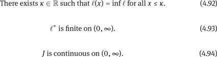
Note that these assumptions imply that ∗(0) < ∞ and that J(0+) ≥ κ. Moreover, J(z) increases to +∞ as z ↑ ∞, and hence so does (J(z)). Since

it follows from (4.89) that

These facts and the continuity of J imply that for large enough n there exists some λn > 0 such that

Let us define

Then Xn is bounded and belongs to A . Hence, it follows from (4.89) and (4.95) that

Since we assumed that αmin(Q) < ∞, the decreasing limit λ∞ of λn must be strictly positive. The fact that ∗ is bounded from below allows us to apply Fatou’s lemma:

This proves (4.91) under the assumptions (4.92), (4.93), and (4.94).

If (4.92) and (4.93) hold, but J is not continuous, then we can approximate the upper semicontinuous function J from above with an increasing continuous function on [0,∞) such that

satisfies

Let := ∗∗ denote the Fenchel–Legendre transform of ∗. Since ∗∗ = by Proposition A.9, it follows that

Therefore,

Since we already know that the assertion holds for , we get that

By letting ε ↓ 0, we obtain (4.91).

Finally, we remove conditions (4.92) and (4.93). If ∗(z) = +∞ for some z, then z must be an upper bound for the slope of . So we will approximate by a sequence (n)of convex loss functions whose slope is unbounded. Simultaneously, we can handle the case where does not take on its infimum. To this end, we choose a sequence κn ↓ inf such that κn ≤ (0) < x0. We can define, for instance,

Then n decreases pointwise to . Each loss function n satisfies (4.92) and (4.93).

Hence, for any ε > 0 there are such that

where is the penalty function arising from n. Note that by Lemma 4.116. Our assumption αmin(Q) < ∞, the fact that

and part (c) of Lemma 4.117 show that the sequence must be bounded away from zero and from infinity. Therefore, we may assume that converges to some Using again the fact that uniformly in n and z, Fatou’s lemma yields

This completes the proof of the theorem.

Example 4.118. Take

where p > 1. Then

where q = p/(p − 1) is the usual dual coefficient. We may apply Theorem 4.115 for any x0 > 0. Let Q ∈ M1(P) with density φ := dQ/dP. Clearly, αmin(Q) = +∞ if φ / ∈ Lq(Ω,F, P). Otherwise, the infimum in (4.88) is attained for

Hence, we can identify αmin(Q) for any Q P as

Taking the limit p ↓ 1, we obtain the case (x) = x+ where we measure the risk in terms of the expected shortfall. Here we have

◊

Together with Proposition 4.20, Theorem 4.115 yields the following result for risk measures which are defined in terms of a robust notion of bounded shortfall risk. Here it is convenient to define ∗(∞) := ∞.

Corollary 4.119. Suppose that Qis a family of probability measures on (Ω,F), and that , ∗, and x0 are as in Theorem 4.115. We define a set of acceptable positions by

Then the corresponding convex risk measure can be represented in terms of the penalty function

where dQ/dP is the density appearing in the Lebesgue decomposition of Q with respect to P as in Theorem A.17.

Example 4.120. In the case of Example 4.114, the corresponding robust problem in Corollary 4.119 leads to the following entropy minimization problem: For a given Q and a set Q of probability measures, find

Note that this problem is different from the standard problem of minimizing H (Q|P) with respect to the first variable Q as it appears in Section 3.2.

◊

Example 4.121. Take x0 = 0 in (4.83) and (x) := x. Then

Therefore, α(Q) = ∞ if Q ≠ P, and ρ(X) = E[ −X ]. If Q is a set of probability measures, the “robust” risk measure ρ of Corollary 4.119 is coherent, and it is given by

◊

Exercise 4.9.3. Consider a situation in which model uncertainty is described by a parametric family Pθ for θ ∈ Θ. In each model Pθ, the expected utility of a random variable X ∈ X is Eθ[ u(X) ],where u : ℝ → ℝ is a given utility function. In a Bayesian approach, one would choose a prior distribution μ on Θ. In terms of F. Knight’s distinction between risk and uncertainty, we would now be in a situation of model risk. Risk neutrality with respect to this model risk would be described by the utility functional

here we assume that is sufficiently measurable. In order to capture model risk aversion, we could choose another utility function û : ℝ → ℝ and consider the utility functional Û(X) defined by

Show that Û is quasi-concave, i.e.,

Show next that for û(x) = 1 − e−αx, the utility functional Û(X) takes the form Û(X) = −ρ(u(X)) for a convex risk measure ρ. Then compute the minimal penalty function in the robust representation of ρ (here you may assume that Θ is a finite set). Discuss the limit α ↑ ∞.

◊

We now explore the relations between shortfall risk and the divergence risk measures introduced in Example 4.36. To this end, let g : [0,∞[→ ℝ ∪ {+∞} be a lower semicontinuous convex function satisfying g(1) < ∞ and the superlinear growth condition g(x)/x → +∞ as x ↑ ∞. Recall the definition of the g-divergence,

and of the corresponding divergence risk measure

We have seen in Exercise 4.3.4 that ρ is continuous from below and that Ig( · |P) is its minimal penalty function, so the supremum in (4.97) is actually a maximum. The following representation for ρg extends the corresponding result for AV@R in Proposition 4.51, where g = ∞· (1/λ,∞) .

Theorem 4.122. Let g∗(y) = supx>0(xy − g(x)) be the Fenchel–Legendre transform of g. Then

The proof of Theorem 4.122 is based on Theorem 4.115. In fact, we will see that, in some sense, the two representation (4.88) and (4.98) are dual with respect to each other. We prepare the proof with the following exercises. The first one concerns a nice and sometimes very useful property of convex functions.

Exercise 4.9.4. If h is a convex function on [0,∞), then

is a convex function of (x, y) ∈ (0,∞) × [0,∞).

◊

Exercise 4.9.5. Let g : [0,∞[→ ℝ ∪{+∞} be a lower semicontinuous convex function satisfying g(1) < ∞ and the superlinear growth condition g(x)/x → +∞ as x ↑ ∞. For λ > 0 let gλ(x) := λg(x/λ). Then is convex by Exercise 4.9.4. Let γλ(Q) = Igλ (Q|P) be the corresponding gλ-divergence. Show that is a convex functional and that

is a lower semicontinuous convex function in λ if X ∈ L∞ is fixed.

◊

Proof of Theorem 4.122. Let gλ and h be as in Exercise 4.9.5. Our aim is to compute h(1). The idea is to use Theorem 4.115 so as to identify the Fenchel–Legendre transform h∗ of h. To this end, we first observe that := g∗ satisfies the assumptions of Theorem 4.115. Next, ∗ = g∗∗ = g by Proposition A.9. Hence, Theorem 4.115 yields that

for all x in the interior of g∗(ℝ), which coincides with the interior of dom f . Exercise 4.9.5 hence yields h(1) = h∗∗(1) = supx(x − f (−x)). We have seen in the proof of Proposition 4.113 that x = −E[ g∗(−f (−x) − X) ] whenever −x belongs to the interior of g∗(ℝ). Hence,

and the assertion follows by noting that the range of f contains all points to the left of where x0 is the lower bound for all points in which the right-hand derivative of g∗ is strictly positive.