1.3Derivative securities

In real financial markets, not only the primary assets are traded. There is also a large variety of securities whose payoff depends in a nonlinear way on the primary assets S0, S1, . . . , Sd, and sometimes also on other factors. Such financial instruments are usually called options, contingent claims, derivative securities, or just derivatives.

Example 1.20. Under a forward contract, one agent agrees to sell to another agent an asset at time 1 for a price K which is specified at time 0. Thus, the owner of a forward contract on the ith asset gains the difference between the actual market price Si and the delivery price K if Si is larger than K at time 1. If Si < K, the owner loses the amount K − Si to the issuer of the forward contract. Hence, a forward contract corresponds to the random payoff

◊

Example 1.21. The owner of a call option on the ith asset has the right, but not the obligation, to buy the ith asset at time 1 for a fixed price K, called the strike price. This corresponds to a payoff of the form

Conversely, a put option gives the right, but not the obligation, to sell the asset at time 1 for a strike price K. The corresponding random payoff is given by

Call and put options with the same strike K are related through the formula

Hence, if the price π(Ccall) of a call option has already been fixed, then the price π(Cput) of the corresponding put option is determined by linearity through the put-call parity

◊

Example 1.22. An option on the value of a portfolio of several risky assets is sometimes called a basket or index option. For instance, a basket call would be of the form (V − K)+. The asset on which the option is written is called the underlying asset or just the underlying.

◊

Put and call options can be used as building blocks for a large class of derivatives.

Example 1.23. A straddle is a combination of “at-the-money” put and call options on a portfolio V = · S, i.e., on put and call options with strike K = π(V):

Thus, the payoff of the straddle increases proportionally to the change of the price of between time 0 and time 1. In this sense, a straddle is a bet that the portfolio price will move, no matter in which direction.

◊

Example 1.24. The payoff of a butterfly spread is of the form

where K > 0 and where is the price of a given portfolio or the value of a stock index. Clearly, the payoff of the butterfly spread is maximal if V = π(V) and decreases if the price at time 1 of the portfolio deviates from its price at time 0. Thus, the butterfly spread is a bet that the portfolio price will stay close to its present value.

◊

Exercise 1.3.1. Draw the payoffs of put and call options, a straddle, and a butterfly spread as functions of its underlying.

◊

Exercise 1.3.2. Consider a butterfly spread as in Example 1.24 and write its payoff as a combination of

(a) call options,

(b) put options

on the underlying. As in the put-call parity (1.11), such a decomposition determines the price of a butterfly spread once the prices of the corresponding put or call options have been fixed.

◊

Example 1.25. The idea of portfolio insurance is to increase exposure to rising asset prices, and to reduce exposure to falling prices. This suggests to replace the payoff of a given portfolio by a modified profile h(V), where h is convex and increasing. Let us first consider the case where V ≥ 0. Then the corresponding payoff h(V) can be expressed as a combination of investments in bonds, in V itself, and in basket call options on V. To see this, recall that convexity implies that

for the increasing right-hand derivative hʹ := hʹ+ of h; see Appendix A.1. By the arguments in Lemma A.23, the increasing right-continuous function hʹ can be represented as the distribution function of a positive Radon measure γ on [0,∞). That is, hʹ(x) = γ([0, x]) for x ≥ 0. Recall that a positive Radon measure is a σ-additive measure that assigns to each Borel set A ⊂ [0,∞) a value in γ(A) ∈ [0,∞], which is finite if A is compact. An example is the Lebesgue measure on [0, ∞). Using the representation hʹ(x) = γ([0, x]) in (1.12), Fubini’s theorem implies that

Since the inner integral equals (x − z)+, we obtain

◊

The formula (1.13) yields a representation of h(V) in terms of investments in bonds, in itself, and in call options on V. It requires, however, that V is nonnegative and that both h(0) and hʹ(0) are finite. Also, it is sometimes more convenient to have a development around the initial value of the portfolio than to have a development around zero. Corresponding extensions of formula (1.13) are explored in the following exercise.

Exercise 1.3.3. In this exercise, we consider the situation of Example 1.25 without insisting that the payoff takes only nonnegative values. In particular, the portfolio may also contain short positions. We assume that is a continuous function.

(a) Show that for convex h there exists a nonnegative Radon measure γ on ℝ such that the payoff h(V) can be realized by holding bonds, forward contracts, and a mixture of call and put options on V:

Note that the put and call options occurring in this formula are “out of the money” in the sense that their “intrinsic value”, i.e., their value when V is replaced by its present value πV, is zero.

(b) Now let h be any twice continuously differentiable function on ℝ. Deduce from part (a) that

In fact, this formula is nothing but a first-order Taylor formula where the remainder term is expressed in integral form.

◊

Example 1.26. A reverse convertible bond pays interest which is higher than that earned by an investment into the riskless bond. But at maturity t = 1, the issuer may convert the bond into a predetermined number of shares of a given asset Si instead of paying the nominal value in cash. The purchase of this contract is equivalent to the purchase of a standard bond and the sale of a certain put option. More precisely, suppose that 1 is the price of the reverse convertible bond at t = 0, that its nominal value at maturity is 1 + , and that it can be converted into x shares of the ith asset. This conversion will happen if the asset price Si is below K := (1+)/x. Thus, the payoff of the reverse convertible bond is equal to

i.e., the purchase of this contract is equivalent to a risk-free investment of the amount (1 + )/(1 + r) with interest r and the sale of the put option x(K − Si)+ for the price ( − r)/(1 + r).

◊

Example 1.27. A discount certificate on pays off the amount

where the number K > 0 is often called the cap. Since

buying the discount certificate is the same as purchasing and selling the basket call option Ccall := (V − K)+. If the price π(Ccall) has already been fixed, then the price of C is given by Hence, the discount certificate is less expensive than the portfolio itself, and this explains the name. On the other hand, it participates in gains of only up to the cap K.

◊

Example 1.28. For an insurance company, it may be desirable to shift some of its insurance risk to the financial market. As an example of such an alternative risk transfer, consider a catastrophe bond issued by an insurance company. The interest paid by this security depends on the occurrence of certain special events. For instance, the contract may specify that no interest will be paid if more than a given number of insured cars are damaged by hail on a single day during the lifetime of the contract; as a compensation for taking this risk, the buyer will be paid an interest above the usual market rate if this event does not occur.

◊

Mathematically, it will be convenient to focus on contingent claims whose payoff is nonnegative. Such a contingent claim will be interpreted as a contract which is sold at time 0 and which pays a random amount C(ω) ≥ 0 at time 1. A derivative security whose terminal value may also become negative can usually be reduced to a combination of a nonnegative contingent claim and a short position in some of the primary assets S0, S1, . . . , Sd. For instance, the terminal value of a reverse convertible bond is bounded from below so that it can be decomposed into a short position in cash and into a contract with positive value. From now on, we will work with the following formal definition of the term “contingent claim”.

Definition 1.29. A contingent claim is a random variable C on the underlying probability space (Ω,F, P) such that

A contingent claim C is called a derivative of the primary assets S0, . . . , Sd if it is measurable with respect to the σ-field σ(S0, . . . , Sd) generated by the assets, i.e., if

for a measurable function f on

◊

So far, we have only fixed the prices πi of our primary assets Si. Thus, it is not clear what the correct price should be for a general contingent claim C. Our main goal in this section is to identify those possible prices that are compatible with the given prices in the sense that they do not generate arbitrage. Our approach is based on the observation that trading C at time 0 for a price πC corresponds to introducing a new asset with the prices

Definition 1.30. A real number πC ≥ 0 is called an arbitrage-free price of a contingent claim C if the market model extended according to (1.14) is arbitrage-free. The set of all arbitrage-free prices for C is denoted Π(C).

◊

In the previous definition, we made the implicit assumption that the introduction of a contingent claim C as a new asset does not affect the prices of primary assets. This assumption is reasonable as long as the traded volume of C is small compared to that of the primary assets. In Section 3.6 we will discuss the equilibrium approach to asset pricing, where an extension of the market will typically change the prices of all traded assets.

The following result shows in particular that we can always find an arbitrage-free price for a given contingent claim C if the initial model is arbitrage-free.

Theorem 1.31. Suppose that the set P of equivalent risk-neutral measures for the original market model is nonempty. Then the set of arbitrage-free prices of a contingent claim C is nonempty and given by

Proof. By Theorem 1.7, πC is an arbitrage-free price for C if and only if there exists an equivalent risk-neutral measure for the market model extended via (1.14), i.e.,

In particular, is necessarily contained in P, and we obtain the inclusion ⊆ in (1.15). Conversely, if πC = E∗[ C /(1 + r) ] for some P∗ ∈ P, then this P∗ is also an equivalent risk-neutral measure for the extended market model, and so the two sets in (1.15) are equal.

To show that Π(C) is nonempty, we first fix some measure ≈ P such that [ C ] < ∞. For instance, we can take d= c(1 + C)−1dP, where c is the normalizing constant. Under , the market model is arbitrage-free. Hence, Theorem 1.7 yields P∗ ∈ P such that dP∗/dis bounded by some constant λ. In particular,

It follows that E∗[ C/(1 + r) ] ∈ Π(C).

Exercise 1.3.4. Show that the set Π(C) of arbitrage-free prices of a contingent claim is convex and hence an interval.

◊

The following theorem provides a dual characterization of the lower and upper bounds

which are often called arbitrage bounds for C.

Theorem 1.32. In an arbitrage-free market model, the arbitrage bounds of a contingent claim C are given by

and

Proof. We only prove the identities for the upper arbitrage bound. The ones for the lower bound are obtained in a similar manner; see Exercise 1.3.5. Let M denote the set of all m ∈ [0,∞] for which there exists ξ ∈ ℝd such that m + ξ · Y ≥ C/(1 + r) P-almost surely. Taking the expectation with P ∗ ∈ P on both sides of the inequality yields m ≥ E∗[ C/(1 + r) ]. This implies

where we have used Theorem 1.31 in the last identity.

Next we show that all inequalities in (1.17) are in fact identities. This is trivial if πsup(C) = ∞. For πsup(C) < ∞, we will show that m > πsup(C) implies m ≥ inf M. By definition, πsup(C) < m < ∞ requires the existence of an arbitrage opportunity in the market model extended by πd+1 := m and Sd+1 := C. That is, there is (ξ , ξ d+1) ∈ ℝd+1 such that ξ·Y+ξ d+1(C/(1+r)−m) is almost-surely nonnegative and strictly positive with positive probability. Since the original market model is arbitrage-free, ξ d+1 is nonzero. In fact, we must have ξ d+1 < 0, as taking expectations with respect to some P∗ ∈ P with E∗[ C ] < ∞yields

and the term in parenthesis is negative since m > πsup(C). Thus, we may define ζ := −ξ /ξ d+1 ∈ ℝd and obtain m + ζ · Y ≥ C/(1 + r) P-a.s., hence m ≥ inf M.

We now prove that inf M belongs to M. This is clear if inf M = ∞, so we only need to consider the case in which inf M < ∞. We may assume without loss of generality that the market model is nonredundant in the sense of Definition 1.15. For a sequence mn ∈ M that decreases towards inf M = πsup(C), we fix ξn ∈ ℝd such that mn + ξn · Y ≥ C/(1 + r) P-almost surely. If lim infn |ξn| < ∞, there exists a subsequence of (ξn) that converges to some ξ ∈ ℝd. Passing to the limit yields πsup(C) + ξ · Y ≥ C/(1 + r) P-a.s., which gives πsup(C) ∈ M. But this is already the desired result, since the following argument will show that the case lim infn |ξn| = ∞ cannot occur. Indeed, after passing to some subsequence if necessary, ηn := ξn/|ξn| converges to some η ∈ ℝd with |η| = 1. Under the assumption that |ξn|→ ∞, passing to the limit in

yields η · Y ≥ 0. The absence of arbitrage opportunities thus implies η · Y = 0 P-a.s., whence η = 0 by nonredundance of the model. But this contradicts the fact that |η| = 1.

Exercise 1.3.5. Prove the identity (1.16).

◊

Remark 1.33. Theorem 1.32 shows that πsup(C) is the lowest possible price of a portfolio with

Such a portfolio is often called a “superhedging strategy” or “superreplication” of C, and the identities for πinf(C) and πsup(C) obtained in Theorem 1.32 are often called superhedging duality relations. When using , the seller of C would be protected against any possible future claims of the buyer of C. Thus, a natural goal for the seller would be to finance such a superhedging strategy from the proceeds of C. Conversely, the objective of the buyer would be to cover the price of C from the sale of a portfolio η with

which is possible if and only if Unless C is an attainable payoff, however, neither objective can be fulfilled by trading C at an arbitrage-free price, as shown in Corollary 1.35 below. Thus, any arbitrage-free price involves a trade-off between these two objectives.

◊

For a portfolio the resulting payoff if positive, may be viewed as a contingent claim, and in particular as a derivative. Those claims which can be replicated by a suitable portfolio will play a special role in the sequel.

Definition 1.34. A contingent claim C is called attainable (replicable, redundant) if P-a.s. for some Such a portfolio strategy is then called a replicating portfolio for C.

◊

If one can show that a given contingent claim C can be replicated by some portfolio , then the problem of determining a price for C has a straightforward solution: The price of C is unique and equal to the cost of its replication, due to the law of one price. The following corollary shows in particular that the attainable contingent claims are in fact the only ones that admit a unique arbitrage-free price.

Corollary 1.35. Suppose the market model is arbitrage-free and C is a contingent claim.

(a) C is attainable if and only if it admits a unique arbitrage-free price.

(b) If C is not attainable, then πinf(C) < πsup(C) and

Proof. To prove part (a), note first that |Π(C)| = 1 if C is attainable. The converse implication will follow from (b).

In order to prove part (b), note first that Π(C) is an interval due to Exercise 1.3.4. To show that this interval is open, it suffices to exclude the possibility that it contains one of its boundary points πinf(C) and πsup(C). To this end, we use Theorem 1.32 to find ξ ∈ ℝd such that

Since C is not attainable, this inequality cannot be an almost-sure identity. Hence, with ξ0 := π · ξ − πinf(C), the strategy (ξ0, −ξ, 1) ∈ ℝd+2 is an arbitrage opportunity in the market model extended by πd+1 := πinf(C) and Sd+1 := C. Therefore πinf(C) is not an arbitrage-free price for C. The possibility πsup(C) ∈ Π(C) is excluded by a similar argument.

Remark 1.36. In Theorem 1.32, the set P of equivalent risk-neutral measures can be replaced by the set of risk-neutral measures that are merely absolutely continuous with respect to P. That is,

for any contingent claim C. To prove this, note first that P ⊂ , so that we get the two inequalities “≥” and “≤” in (1.18). On the other hand, for ∈ , P∗ ∈ P with E∗[ C ] < ∞, and ε ∈ (0, 1], the measure belongs to P and satisfies Sending ε ↓ 0 yields the converse inequalities.

◊

Remark 1.37. Consider any arbitrage-free market model, and let Ccall = (Si − K)+ be a call option on the ith asset with strike K > 0. Clearly, Ccall ≤ Si so that

for any P∗ ∈ P. From Jensen’s inequality, we obtain the following lower bound:

Thus, the following universal bounds hold for any arbitrage-free market model:

For a put option Cput = (K − Si)+, one obtains the universal bounds

If r ≥ 0, then the lower bound in (1.19) can be further reduced to πinf(Ccall) ≥ (πi − K )+. Informally, this inequality states that the value of the right to buy the ith asset at t = 0 for a price K is strictly less than any arbitrage-free price for Ccall. This fact is sometimes expressed by saying that the time value of a call option is nonnegative. The quantity (πi −K)+ is called the intrinsic value of the call option. Observe that an analogue of this relation usually fails for put options: The left-hand side of (1.20) can only be bounded by its intrinsic value (K − πi)+ if r ≤ 0. If the intrinsic value of a put or call option is positive, then one says that the option is “in the money”. For πi = K one speaks of an “at-the-money” option. Otherwise, the option is “out of the money”.

◊

In many situations, the universal arbitrage bounds (1.19) and (1.20) are in fact attained, as is illustrated by the following example.

Example 1.38. Take any market model with a single risky asset S = S1 such that the distribution of S under P is concentrated on {0, 1, . . . , } with positive weights. Without loss of generality, we may assume that S has under P a Poisson distribution with parameter 1, i.e., S is P-a.s. integer-valued and

If we take r = 0 and π = 1, then P is a risk-neutral measure and so the market model is arbitrage-free. We are going to show that the upper and lower bounds in (1.19) are attained for this model by using Remark 1.36. To this end, consider the measure ∈ which is defined by its density

We get

so that the lower bound in (1.19) is attained, i.e., we have

To see that also the upper bound is sharp, we define

It is straightforward to check that

defines a measure n ∈ such that

By sending n ↑ ∞, we see that also the upper bound in (1.19) is attained:

Furthermore, the put-call parity (1.11) shows that the universal bounds (1.20) for put options are attained as well.

◊

Exercise 1.3.6. We consider the market model from Exercise 1.1.2 and suppose that a < π(1 + r) < b so that the model is arbitrage-free. Let C be a derivative that is given by C = h(S), where h ≥ 0 is a convex function. Show that

◊

Exercise 1.3.7. In an arbitrage-free market model, we consider a derivative C that is given by C = h(S1), where h ≥ 0 is a convex function. Derive the following arbitrage bounds for C:

◊

1.4Complete market models

Our goal in this section is to characterize the particularly transparent situation in which all contingent claims are attainable.

Definition 1.39. An arbitrage-free market model is called complete if every contingent claim is attainable.

◊

The following theorem characterizes the class of all complete market models. It is sometimes called the “second fundamental theorem of asset pricing”.

Theorem 1.40. An arbitrage-free market model is complete if and only if there exists exactly one risk-neutral probability measure, i.e., if | P| = 1.

Proof. If the model is complete, then the indicator A of each set A ∈ F is an attainable contingent claim. Hence, Corollary 1.35 implies that P∗[ A ] = E∗[ A] is independent of P∗ ∈ P. Consequently, there is just one risk-neutral probability measure.

Conversely, suppose that P = {P∗}. If C is a contingent claim, then Theorem 1.31 states that the set Π(C) of arbitrage-free prices is nonempty and given by

Since P has just one element, the same must hold for Π(C). Hence, Corollary 1.35 implies that C is attainable.

We will now show that every complete market model has a finite structure and can be reduced to a finite probability space. To this end, observe first that in every market model the following inclusion holds for each P∗ ∈ P:

see Appendix A.7 for the definition of Lp-spaces. If the market is complete then all of these inclusions are in fact equalities. In particular, F coincides with σ(S1, . . . , Sd) modulo P-null sets, and every contingent claim coincides P-a.s. with a derivative of the traded assets. Since the linear space V is finite-dimensional, it follows that the same must be true of L0(Ω,F, P). But this means that the model can be reduced to a finite number of relevant scenarios. This observation can be made precise by using the notion of an atom of the probability space (Ω,F, P). Recall that a set A ∈ F is called an atom of (Ω,F, P), if P[ A ] > 0 and if each B ∈ F with B ⊆ A satisfies either P[ B ] = 0 or P[ B ] = P[ A ].

Proposition 1.41. For p ∈ [0,∞], the dimension of the linear space Lp(Ω,F, P) is given by

Moreover, n := dim Lp(Ω,F, P) < ∞ if and only if there exists a partition of Ω into n atoms of (Ω,F, P).

Proof. Suppose that there is a partition A1, . . . , An of Ω such that Ai ∈ F and P[ Ai ] > 0. The corresponding indicator functions A1 , . . . , An can be regarded as linearly independent vectors in Lp := Lp(Ω,F, P). Thus dim Lp ≥ n. Consequently, it suffices to consider only the case in which the right-hand side of (1.22) is a finite number, say n0. If A1, . . . , An0 is a corresponding partition, then each Ai is an atom because otherwise n0 would not be maximal. Thus, any Z ∈ Lp is P-a.s. constant on each Ai. If we denote the value of Z on Ai by zi, then

Hence, the indicator functions A1 , . . . , An0 form a basis of Lp, and this implies dim Lp = n0.

Since for a complete market model the inclusions in (1.21) are in fact equalities, we have

with equality if the model is nonredundant. Together with Proposition 1.41, this implies the following result on the structure of complete market models.

Corollary 1.42. For every complete market model there exists a partition of Ω into at most d + 1 atoms of (Ω,F, P).

Example 1.43. Consider the simple situation where the sample space Ω consists of two elements ω+ and ω−, and where the measure P is such that

We assume that there is one single risky asset, which takes at time t = 1 the two values b and a with the respective probabilities p and 1 − p, where a and b are such that 0 ≤ a < b:

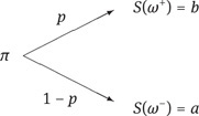
This model does not admit arbitrage if and only if

see also Example 1.10. In this case, the model is also complete: Any risk-neutral measure P∗ must satisfy

and this condition uniquely determines the parameter p∗ = P∗[ {ω+} ] as

Hence |P| = 1, and completeness follows from Theorem 1.40. Alternatively, we can directly verify completeness by showing that a given contingent claim C is attainable if (1.23) holds. Observe that the condition

is a system of two linear equations for the two real variables ξ0 and ξ. The solution is given by

Therefore, the unique arbitrage-free price of C is

For a call option C = (S − K)+ with strike K ∈ [a, b], we have

Note that this price is independent of p and increasing in r, while the classical discounted expectation with respect to the “objective” measure P,

is decreasing in r and increasing in p.

In this example, one can illustrate how options can be used to modify the risk of a position. Consider the particular case in which the risky asset can be bought at time t = 0 for the price π = 100. At time t = 1, the price is either S(ω+) = b = 120 or S(ω−) = a = 90, both with positive probability. If we invest in the risky asset, the corresponding returns are given by

Now consider a call option C := (S − K)+ with strike K = 100. Choosing r = 0, the price of the call option is

from formula (1.24). Hence the return

on the initial investment π(C) equals

or

according to the outcome of the market at time t = 1. Here we see a dramatic increase of both profit opportunity and risk; this is sometimes referred to as the leverage effect of options.

On the other hand, we could reduce the risk of holding the asset by holding a combination

of a put option and the asset itself. This “portfolio insurance” will of course involve an additional cost. If we choose our parameters as above, then the put-call parity (1.11) yields that the price of the put option (K − S)+ is equal to 20/3. Thus, in order to hold both S and a put, we must invest the capital 100 + 20/3 at time t = 0. At time t = 1, we have an outcome of either 120 or of 100 so that the return of is given by

◊

Exercise 1.4.1. We consider the following three market models.

(A) Ω = {ω1, ω2} with and one risky asset with prices

(B) Ω = {ω1, ω2, ω3} with and one risky asset with prices

(C) Ω = {ω1, ω2, ω3} with and two risky assets with prices

Each of these models is endowed with a probability measure that assigns strictly positive probability to each element of the corresponding sample space Ω.

(a) Which of these models are arbitrage-free? For those that are, describe the set P of equivalent risk-neutral measures. For those that are not, find an arbitrage opportunity.

(b) Discuss the completeness of those models that are arbitrage-free. For those that are not complete find nonattainable contingent claims.

◊

Exercise 1.4.2. Let Ω = {ω1, ω2, ω3} be endowed with a probability measure P such that P[{ωi}] > 0 for i = 1, 2, 3 and consider the market model with r = 0 and one risky asset with prices π1 = 1 and 0 < S1(ω1) < S1(ω2) < S1(ω3).We suppose that the model is arbitrage-free.

(a) Describe the following objects as subsets of three-dimensional Euclidean space ℝ3:

(i) the set P of equivalent risk neutral measures;

(ii) the set of absolutely continuous risk neutral measures;

(iii) the set of attainable contingent claims.

(b) Find an example for a nonattainable contingent claim.

(c) Show that the supremum

is attained for every contingent claim C.

(d) Let C be a contingent claim. Give a direct and elementary proof of the fact that the map that assigns to each ∈ the expectation [ C ] is constant if and only if the supremum (1.25) is attained in some element of P.

◊

Exercise 1.4.3. Let Ω = {ω1, . . . , ωN} be endowed with a probability measure P such that P[{ωi}] > 0 for i = 1, . . . , N. On this probability space we consider a market model with interest rate r = 0 and with one risky asset whose prices satisfy π1 = 1 and

Show that there are strikes K1, . . . , K N−2 > 0 and prices πKi such that the corresponding call options (S1 − Ki)+ complete the market in the following sense: the market model extended by the risky assets with prices

is arbitrage-free and complete.

◊

Exercise 1.4.4. Let Ω = {ω1, . . . , ωN+1} be endowed with a probability measure P such that P[{ωi}] > 0 for i = 1, . . . , N + 1.

(a) On this probability space we consider a nonredundant and arbitrage-free market model with d risky assets and prices and where d < N. Show that this market model can be extended by additional assets with prices πd+1, . . . , πN and Sd+1, . . . , SN in such a way that the extended market model is arbitrage-free and complete.

(b) Let specifically N = 2, d = 1, π1 = 2, and

We suppose furthermore that the risk-free interest rate r is chosen such that the model is arbitrage-free. Find a nonattainable contingent claim. Then find an extended model that is arbitrage-free and complete. Finally determine the unique equivalent risk-neutral measure P∗ in the extended model.

◊