
10Minimizing the hedging error
In this chapter, we present an alternative approach to the problem of hedging in an incomplete market model. Instead of controlling the downside risk, we simply aim at minimizing the quadratic hedging error. We begin with a local version of the minimization problem, which may be viewed as a sequential regression procedure. Its solution involves an orthogonal decomposition of a given contingent claim; this extends a classical decomposition theorem for martingales known as the Kunita–Watanabe decomposition. Often, the value process generated by a locally risk-minimizing strategy can be described as the martingale of conditional expectations of the given contingent claim for a special choice of an equivalent martingale measure. Such “minimal” martingale measures will be studied in Section 10.2. In Section 10.3, we investigate the connection between local risk minimization and the problem of variance-optimal hedging where one tries to minimize the global quadratic hedging error. The local and the global versions coincide if the underlying measure is itself a martingale measure.
10.1Local quadratic risk
In this section, we no longer restrict our discussion to strategies which are self-financing. Instead, we admit the possibility that the value of a position is readjusted at the end of each period by an additional investment in the numéraire asset. This means that, in addition to the initial investment at time t = 0, we allow for a cash flow throughout the trading periods up to the final time T. In particular, it will now be possible to replicate any given European claim, simply by matching the difference between the payoff of the claim and the value generated by the preceding strategy with a final transfer at time T.
Definition 10.1. A generalized trading strategy is a pair of two stochastic process (ξ0, ξ) such that ![]() is adapted, and such that ξ = (ξt)t=1,...,T is a d-dimensional predictable process. The (discounted) value process V of (ξ0, ξ) is defined as
is adapted, and such that ξ = (ξt)t=1,...,T is a d-dimensional predictable process. The (discounted) value process V of (ξ0, ξ) is defined as
◊
For such a generalized trading strategy (ξ0, ξ), the gains and losses accumulated up to time t by investing into the risky assets are given by the sum
The value process V takes the form
if and only if ![]() is a self-financing trading strategy with initial investment
is a self-financing trading strategy with initial investment ![]() In this case,
In this case, ![]() is a predictable process. In general, however, the difference
is a predictable process. In general, however, the difference
is now nontrivial, and it can be interpreted as the cumulative cost up to time t. This motivates the following definition.
Definition 10.2. The gains process G of a generalized trading strategy (ξ0, ξ) is given by
The cost process C of (ξ0, ξ) is defined as the difference
of the value process V and the gains process G.
◊
In this and in the following sections, we will measure the risk of a strategy in terms of quadratic criteria for the hedging error, based on the “objective” measure P. Our aim will be to minimize such criteria within the class of those generalized strategies (ξ0, ξ) which replicate a given discounted European claim H in the sense that their value process satisfies
The claim H will be fixed for the remainder of this section. As usual we assume that the σ-field F0 is trivial, i.e., F0 = {∅, Ω}. In contrast to the previous sections of Part II, however, our approach does not exclude a priori the existence of arbitrage opportunities, even though the interesting cases will be those in which there exist equivalent martingale measures. Since our approach is based on L2-techniques, another set of hypotheses is needed:
Assumption 10.3. Throughout this section, we assume that the discounted claim H and the discounted price process X of the risky assets are both square-integrable with respect to the objective measure P:
(a) H ∈ L2(Ω,FT , P) =: L2(P).
(b) Xt ∈ L2(Ω,Ft , P;ℝd) for all t.
In addition to these assumptions, the quadratic optimality criteria we have in mind require the following integrability conditions for strategies.
Definition 10.4. An L2-admissible strategy for H is a generalized trading strategy (ξ0, ξ) whose value process V satisfies
and whose gains process G is such that
◊
We can now introduce the local version of a quadratic criterion for the hedging error of an L2-admissible strategy.
Definition 10.5. The local risk process of an L2-admissible strategy (ξ0, ξ) is the process
An L2-admissible strategy ![]() is called a locally risk-minimizing strategy if, for all t,
is called a locally risk-minimizing strategy if, for all t,
for each L2-admissible strategy (ξ0, ξ) whose value process satisfies ![]()
![]()
◊
Remark 10.6. The reason for fixing the value Vt+1 = ÛVt+1 in the preceding definition becomes clear when we try to construct a locally risk-minimizing strategy (![]() 0,
0, ![]() ) backwards in time. At time T, we want to construct
) backwards in time. At time T, we want to construct ![]() as a minimizer for the local risk
as a minimizer for the local risk ![]() Since the terminal value of every L2-admissible strategy must be equal to H, this minimization requires the side
Since the terminal value of every L2-admissible strategy must be equal to H, this minimization requires the side ![]()
As we will see in the proof of Theorem 10.9 below, minimality of completely determines and ![]() T and ÛV1, but one is still free to choose and
T and ÛV1, but one is still free to choose and ![]() T−among all with In the next step, it is therefore natural to minimize
T−among all with In the next step, it is therefore natural to minimize ![]() under the condition that VT−1 is equal to the value ÛVT−1 obtained from the preceding step. Moreover, the problem will now be of the same type as the previous one.
under the condition that VT−1 is equal to the value ÛVT−1 obtained from the preceding step. Moreover, the problem will now be of the same type as the previous one. ![]()
![]()
![]() T−
T−![]()
![]() 1
1
◊
Although locally risk-minimizing strategies are generally not self-financing, it will turn out that they are “self-financing on average” in the following sense:
Definition 10.7. An L2-admissible strategy is called mean self-financing if its cost process C is a P-martingale, i.e., if
◊
In order to formulate conditions for the existence of a locally risk-minimizing strategy, let us first introduce some notation. The conditional covariance of two random variables W and Z with respect to P is defined as
provided that the conditional expectations and their difference make sense. Moreover, if Z = (Z1, . . . , Zd) is a random vector and W is a scalar random variable, then cov(W, Z | Ft ) will be understood in a component-wise manner. That is, cov(W, Z | Ft ) is the vector with components cov(W, Zi | Ft ), i = 1, . . . , d. We also define the conditional variance of W under P as
see also Exercise 5.2.6.
Definition 10.8. Two adapted processes U and Y are called strongly orthogonal with respect to P if the conditional covariances
are well-defined and vanish P-almost surely.
◊
When we consider the strong orthogonality of two processes U and Y in the sequel, then usually one of them will be a P-martingale. In this case, the conditional covariances of their increments reduce to
After these preparations, we are now ready to state our first result, namely the following characterization of locally risk-minimizing strategies.
Theorem 10.9. An L2-admissible strategy is locally risk-minimizing if and only if it is mean self-financing and its cost process is strongly orthogonal to X.
Proof. The local risk process of any L2-admissible strategy (ξ0, ξ) can be expressed as a sum of two nonnegative terms:
Since the conditional variance does not change if we add Ft-measurable random variables to its argument, the first term on the right-hand side takes the form
The second term satisfies
In a second step, we fix t and Vt+1, and we consider ξt+1 and Vt as parameters. Our purpose is to derive necessary conditions for the minimality of ![]() with respect to variations of ξt+1 and Vt. To this end, note first that it is possible to change the parameters
with respect to variations of ξt+1 and Vt. To this end, note first that it is possible to change the parameters ![]() and ξt in such away that Vt takes any given value, that the modified strategy is still an L2-admissible strategy for H, and that the values of ξt+1 and Vt+remain unchanged. In particular, the value in (1 10.2
and ξt in such away that Vt takes any given value, that the modified strategy is still an L2-admissible strategy for H, and that the values of ξt+1 and Vt+remain unchanged. In particular, the value in (1 10.2![]() ) is not affected by such a modification, and so it is necessary for the optimality of that Vt minimizes (10.3). This is the case if and only if
) is not affected by such a modification, and so it is necessary for the optimality of that Vt minimizes (10.3). This is the case if and only if
The value of (10.2) is independent of Vt and a quadratic form in terms of the Ft-measurable random vector ξt+1. Thus, (10.2) is minimal if and only if ξt+1 solves the linear equation
Note that (10.4) is equivalent to
Moreover, given (10.4), the condition (10.5) holds if and only if
where we have used the fact that the conditional covariance in (10.5) is not changed by subtracting the Ft-measurable random variable Vt from the first argument. Backward induction on t concludes the proof.
The previous proof provides a recipe for a recursive construction of a locally risk-minimizing strategy: If Vt+1 is already given, minimize
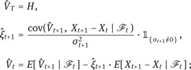
with respect to Vt and ξt+1. This is just a conditional version of the standard problem of determining the linear regression of Vt+1 on the increment Xt+1 − Xt. Let us now consider the case
where our market model contains just one risky asset. Then a heuristic computation yields the following recursive scheme for a solution of our minimization problem:

Here ![]() is a shorthand t2notation for the conditional variance
is a shorthand t2notation for the conditional variance
Defining ![]() we obtain a generalized trading strategy (
we obtain a generalized trading strategy (![]() 0,
0, ![]() ) whose terminal portfolio value ÛVT coincides with H. However, an extra condition is needed to conclude that this strategy is indeed L2-admissible.
) whose terminal portfolio value ÛVT coincides with H. However, an extra condition is needed to conclude that this strategy is indeed L2-admissible.
Proposition 10.10. Consider a market model with a single risky asset and assume that there exists a constant κ such that
Then the recursion (10.6) defines a locally risk-minimizing strategy (ξÛ0, ξÛ).Moreover, any other locally risk-minimizing strategy coincides with (ξÛ0, ξÛ) up to modifications of ξÛt on the set ![]()
Proof. We have to show that (![]() 0,
0, ![]() ξ) is L2-admissible. To this end, observe that the recursion (10.6) and the condition (10.7) imply that
ξ) is L2-admissible. To this end, observe that the recursion (10.6) and the condition (10.7) imply that

The last expectation is finite if ÛVt is square-integrable. In this case, ![]() t · (Xt − Xt−1) ∈ L2(P) and in turn ÛVt−1 ∈ L2(P). Hence, L2-admissibility of (
t · (Xt − Xt−1) ∈ L2(P) and in turn ÛVt−1 ∈ L2(P). Hence, L2-admissibility of (![]() 0,
0, ![]() ) follows by backward induction. The claim that (
) follows by backward induction. The claim that (![]() 0,
0, ![]() ) is locally risk-minimizing as well as the uniqueness assertion follow immediately from the construction.
) is locally risk-minimizing as well as the uniqueness assertion follow immediately from the construction.
Remark 10.11. The predictable process
is called the mean-variance trade-off process of X, and condition (10.7) is known as the assumption of bounded mean-variance trade-off. Intuitively, it states that the forecast E [ X t − Xt−1 | Ft−1 ] of the price increment Xt − Xt−1 is of the same order of magnitude as the corresponding standard deviation σt.
◊
Remark 10.12. The assumption of bounded mean-variance trade-off is equivalent to the existence of some δ < 1 such that
Indeed, with αt = E [ Xt − Xt−1 | Ft−1 ], the assumption of bounded mean-variance trade-off is equivalent to
which is seen to be equivalent to (10.8) by choosing δ = κ/(1 + κ).
◊
Example 10.13. Let us consider a market model consisting of a single risky asset S1 and a riskless bond
with constant return r > −1. We assume that ![]() and that the returns
and that the returns
of the risky asset are independent and identically distributed random variables in L2(P). Under these assumptions, the discounted price process X, defined by
is square-integrable. Denoting by ![]() the mean of Rt and by
the mean of Rt and by ![]() 2 its variance, we get
2 its variance, we get

Thus, the condition of bounded mean-variance trade-off holds without any further assumptions, and a locally risk-minimizing strategy exists. Moreover, P is a martingale measure if and only if ![]() = r.
= r.
◊
Let us return to our general market model with an arbitrary number of risky assets
The following result characterizes the existence of locally risk-minimizing strategies in terms of a decomposition of the claim H.
Corollary 10.14. There exists a locally risk-minimizing strategy if and only if H admits a decomposition
where c is a constant, ξ is a d-dimensional predictable process such that
ξt · (Xt − Xt−1) ∈ L2(P) for all t,
and where L is a square integrable P-martingale which is strongly orthogonal to X and satisfies L0 = 0. In this case, a locally risk-minimizing strategy (![]() 0,
0, ![]() ) is given by
) is given by ![]() = ξ and by the adapted process
= ξ and by the adapted process ![]() 0 defined via
0 defined via ![]() 00 = c and
00 = c and
Proof. If (![]() 0,
0, ![]() ) is agiven locally risk-minimizing strategy with cost process ÛC, then Lt := ÛCt − ÛC0 is a square-integrable P-martingale which is strongly orthogonal to X by Theorem 10.9. Hence, we obtain a decomposition (10.9). Conversely, if such a decomposition exists, then the strategy (
) is agiven locally risk-minimizing strategy with cost process ÛC, then Lt := ÛCt − ÛC0 is a square-integrable P-martingale which is strongly orthogonal to X by Theorem 10.9. Hence, we obtain a decomposition (10.9). Conversely, if such a decomposition exists, then the strategy (![]() 0,
0, ![]() ) has the cost process ÛC= c + L, and Theorem 10.9 implies that (
) has the cost process ÛC= c + L, and Theorem 10.9 implies that (![]() 0,
0, ![]() ) is locally risk-minimizing.
) is locally risk-minimizing.
A decomposition of the form (10.9) will be called an orthogonal decomposition of the contingent claim H with respect to the process X. If X is itself a P-martingale, then the orthogonal decomposition reduces to the Kunita– Watanabe decomposition, which we will explain next. To this end, we will need some preparation.
Lemma 10.15. For two square-integrable martingales M and N, the following two conditions are equivalent:
(a) M and N are strongly orthogonal.
(b) The product MN is a martingale.
Proof. The martingale property of M and N gives
and this expression vanishes if and only if MN is a martingale.
Let H 2 denote the space of all square-integrable P-martingales. Via the identity M t = E [M T | Ft ], each M ∈ H 2 can be identified with its terminal value MT ∈ L2(P). With the standard identification of random variables which coincide P-a.s. (see (A.35)), H 2 becomes a Hilbert space isomorphic to L2(P), if endowed with the inner product
Recall from Definition 6.14 that, for a stopping time τ, the stopped process M τ is defined as
Definition 10.16. A subspace S of H 2 is called stable if Mτ ∈ S for each M ∈ S and every stopping time τ.
◊
Proposition 10.17. For a stable subspace S of H 2 and for L ∈ H 2 with L0 = 0, the following conditions are equivalent.
(a) L is orthogonal to S, i.e.,
(b) L is strongly orthogonal to S, i.e., for each M ∈ S
(c) The product LM is a martingale for each M ∈ S.
Proof. The equivalence of (b) and (c) follows from Lemma 10.15. To prove (a)⇔(c), we will show that LM is a martingale for fixed M ∈ S if and only if ![]() for all stopping times τ ≤ T. By the stopping theorem in the form of Proposition 6.37,
for all stopping times τ ≤ T. By the stopping theorem in the form of Proposition 6.37,
Using the fact that L0M0 = 0 and applying the stopping theorem in the form of Theorem 6.15, we conclude that ![]() for all stopping times τ ≤ T if and only if LM is a martingale.
for all stopping times τ ≤ T if and only if LM is a martingale.
After these preparations, we can now state the existence theorem for the discrete-time version of the Kunita–Watanabe decomposition.
Theorem 10.18. If the process X is a square-integrable martingale under P, then every martingale M ∈ H 2 is of the form
where ξ is a d-dimensional predictable process such that ξt · (Xt − Xt−1) ∈ L2(P) for each t, and where L is a square-integrable P-martingale which is strongly orthogonal to X and satisfies L0 = 0. Moreover, this decomposition is unique in the sense that L is uniquely determined.
Proof. Denote by S the set of all d-dimensional predictable processes ξ such that ξt · (Xt − Xt−1) ∈ L2(P) for each t, and denote by
the “stochastic integral” of ξ ∈ S with respect to X. Since for ξ ∈ S the process G(ξ) is a square-integrable P-martingale, the set G of all those martingales can be regarded as a linear subspace of the Hilbert space H 2. In fact, G is a closed subspace of H 2. To prove this claim, note that the martingale property of G(ξ) implies that
Thus, if ξ(n) is such that G(ξ(n)) is a Cauchy sequence in H 2, then ![]() is a Cauchy sequence in L2(P) for each t. Since P is a
is a Cauchy sequence in L2(P) for each t. Since P is a ![]() martingale measure, we may apply Lemma 1.69 to conclude that any limit point of is of the form ξt · (Xt − Xt−1) for some ξt ∈ L0(Ω,Ft−1, P;ℝd). Hence, G is closed in H 2. Moreover, G is stable. Indeed, if ξ ∈ S and τ is a stopping time, then Gt∧τ(ξ) = Gt(
martingale measure, we may apply Lemma 1.69 to conclude that any limit point of is of the form ξt · (Xt − Xt−1) for some ξt ∈ L0(Ω,Ft−1, P;ℝd). Hence, G is closed in H 2. Moreover, G is stable. Indeed, if ξ ∈ S and τ is a stopping time, then Gt∧τ(ξ) = Gt(![]() ) where
) where
Furthermore, we have ![]() ∈ S since
∈ S since
Since G is closed, the orthogonal projection N of M − M0 onto G is well-defined by standard Hilbert space techniques. The martingale N belongs to G , and the difference L := M − M0 − N is orthogonal to G . By Proposition 10.17, L is strongly orthogonal to G and hence strongly orthogonal to X. Therefore, M = M0 + N + L is the desired decomposition of M.
To show that L is uniquely determined, suppose that there exists another decomposition of M in terms of ![]() and
and ![]() . Then
. Then
is a square-integrable P-martingalewhich is strongly orthogonal to X. By (10.1), strong orthogonality implies
Multiplying this identity with ![]() t − ξt gives
t − ξt gives
and so
In view of ![]() 0 = L0 = 0, we thus get
0 = L0 = 0, we thus get ![]() = L.
= L.
Remark 10.19. In dimension d = 1, the assumption of bounded mean-variance trade-off (10.7) is clearly satisfied if X is a square-integrable P-martingale. Combining Proposition 10.10 with Corollary 10.14 then yields an alternative proof of Theorem 10.18. Moreover, the recursion (10.6) identifies the predictable process ξ appearing in the Kunita–Watanabe decomposition of a martingale M:
◊
10.2Minimal martingale measures
If P is itself a martingale measure, Theorem 10.18 combined with Corollary 10.14 yields immediately a solution to our original problem of constructing locally risk-minimizing strategies:
Corollary 10.20. If P is a martingale measure, then there exists a locally risk-minimizing strategy. Moreover, this strategy is unique in the sense that its value process ÛV is uniquely determined as
and that its cost process is given by
where L is the strongly orthogonal P-martingale arising in the Kunita– Watanabe decomposition of ÛV.
The identity (10.10) allows for a time-consistent interpretation of ÛVt as an arbitrage-free price for H at time t. In the general case in which X is not a martingale under P, one may ask whether there exists an equivalent martingale measure ![]() such that the value process ÛV of a locally risk-minimizing strategy can be obtained in a similar manner as the martingale
such that the value process ÛV of a locally risk-minimizing strategy can be obtained in a similar manner as the martingale
Definition 10.21. An equivalent martingale measure ![]() ∈ P is called a minimal martingale measure if
∈ P is called a minimal martingale measure if
and if every P-martingale M ∈ H 2 which is strongly orthogonal to X is also a -martingale.
◊
The following result shows that a minimal martingale measure provides the desired representation (10.11) – if such a minimal martingale measure exists.
Theorem 10.22. If ![]() is a minimal martingale measure, and if ÛV is the value process of a locally risk-minimizing strategy, then
is a minimal martingale measure, and if ÛV is the value process of a locally risk-minimizing strategy, then
Proof. Denote by
an orthogonal decomposition of H as in Corollary 10.14. Then ÛV is given by
The process L is a ![]() -martingale, because it is a square-integrable P-martingale strongly orthogonal to X.Moreover, ξs ·(Xs−Xs−1) ∈ L1(
-martingale, because it is a square-integrable P-martingale strongly orthogonal to X.Moreover, ξs ·(Xs−Xs−1) ∈ L1(![]() ), because both ξs ·(Xs−Xs−1) and d
), because both ξs ·(Xs−Xs−1) and d![]() /dP are square-integrable with respect to P. It follows that ÛVis a
/dP are square-integrable with respect to P. It follows that ÛVis a ![]() -martingale. In view of ÛVT = H, the assertion follows.
-martingale. In view of ÛVT = H, the assertion follows.
Our next goal is to derive a characterization of a minimal martingale measure and to use it in order to obtain criteria for its existence. To this end, we have to analyze the effect of an equivalent change of measure on the structure of martingales. The results we will obtain in this direction are of independent interest, and their continuous-time analogues have a wide range of applications in stochastic analysis.
Lemma 10.23. Let ![]() be a probability measure equivalent to P. An adapted process
be a probability measure equivalent to P. An adapted process ![]() is a
is a ![]() -martingale if and only if the process
-martingale if and only if the process
is a P-martingale.
Proof. Let us denote
Observe that ![]() t ∈ L1(
t ∈ L1(![]() ) if and only if
) if and only if ![]() tZt ∈ L1(P). Moreover, the process Z is P-a.s. strictly positive by the equivalence of
tZt ∈ L1(P). Moreover, the process Z is P-a.s. strictly positive by the equivalence of ![]() and P. Hence, Proposition A.16 yields that
and P. Hence, Proposition A.16 yields that
and it follows that ![]() [
[ ![]() t+1 | Ft ] =
t+1 | Ft ] = ![]() t if and only if E[
t if and only if E[ ![]() t+1Zt+1 | Ft ] =
t+1Zt+1 | Ft ] = ![]() tZt.
tZt.
The following representation (10.13) of the density process may be viewed as the discrete-time version of the Doléans–Dade stochastic exponential from continuous-time stochastic calculus.
Proposition 10.24. If ![]() is a probability measure equivalent to P, then there exists a P-martingale Λ such that
is a probability measure equivalent to P, then there exists a P-martingale Λ such that
and such that the martingale
Conversely, if Λ is a P-martingale with (10.12) and such that (10.13) defines a P-martingale Z, then
defines a probability measure ![]() ≈ P.
≈ P.
Proof. For ![]() ≈ P given, define Λ by Λ0 = 1 and
≈ P given, define Λ by Λ0 = 1 and
Clearly, (10.13) holds with this choice of Λ. In particular, Λ satisfies (10.12), because the equivalence of P and![]() implies that Zt is P-a.s. strictly positive for all t.
implies that Zt is P-a.s. strictly positive for all t.
In the next step, we show by induction on t that Λt ∈ L1(P). For t = 0 this holds by definition. Suppose that Λt ∈ L1(P). Since Z is nonnegative, the conditional expectation of Z t+1/Zt is well-defined and satisfies P-a.s.
It follows that Zt+1/Z t ∈ L1(P) and in turn that
Now it is easy to derive the martingale property of Λ: Since Zt is strictly positive, we may divide both sides of the equation E[ Zt+1 | Ft ] = Zt by Zt, and we arrive at E[ Λt+1 − Λt | Ft ] = 0.
As for the second part of the assertion, it is clear that E [ Zt ] = Z0 = 1 for all t, provided that Λ is a P-martingale such that (10.12) holds and such that (10.13) defines a strictly positive P-martingale Z.
The following theorem shows how a martingale M is affected by an equivalent change of the underlying probability measure P. Typically, M will no longer be a martingale under the new measure ![]() , and so a nontrivial predictable process (At)t=1,...,T will appear in the Doob decomposition
, and so a nontrivial predictable process (At)t=1,...,T will appear in the Doob decomposition
of M under ![]() . Alternatively, −A may be viewed as the predictable process arising in the Doob decomposition of the
. Alternatively, −A may be viewed as the predictable process arising in the Doob decomposition of the ![]() -martingale
-martingale ![]() under the measure P. The following result, a discrete-time version of the Girsanov formula, describes A in terms of the martingale Λ arising in the representation (10.13) of the successive densities.
under the measure P. The following result, a discrete-time version of the Girsanov formula, describes A in terms of the martingale Λ arising in the representation (10.13) of the successive densities.
Theorem 10.25. Let P and ![]() be two equivalent probability measures, and let Λ denote the P-martingale arising in the representation (10.13) of the successive densities Zt := E[ d
be two equivalent probability measures, and let Λ denote the P-martingale arising in the representation (10.13) of the successive densities Zt := E[ d![]() /dP | Ft ]. If M is a
/dP | Ft ]. If M is a ![]() -martingale such that
-martingale such that ![]() t ∈ L1(P) for all t, then
t ∈ L1(P) for all t, then
is a P-martingale.
Proof. Note first that
According to Lemma 10.23, Z t(![]() t−
t−![]() t−1) is a martingale increment, and hence belongs to L1(P). If we let
t−1) is a martingale increment, and hence belongs to L1(P). If we let
it follows that
In particular, the conditional expectations appearing in the statement of the theorem are P-a.s. well-defined. Moreover, the identity (10.14) implies that P-a.s. on {τn ≥ t}

Thus, we have identified the Doob decomposition of ![]() under P.
under P.
The preceding theorem allows us to characterize those equivalent measures P∗ ≈ P which are martingale measures. Let
denote the Doob decomposition of X under P, where Y is a d-dimensional P-martingale, and (Bt)t=1,...,T is a d-dimensional predictable process given by B0 = 0 and
Corollary 10.26. Let P∗ ≈ P be such that E∗[ |Xt|] < ∞ for each t, and denote by Λ the P-martingale arising in the representation (10.13) of the successive densities Zt := E[ dP∗/dP | Ft ]. Then P∗ is an equivalent martingale measure if and only if the predictable process B in the Doob decomposition (10.15) satisfies

P-a.s. for t = 1, . . . , T.
Proof. If P∗ is an equivalent martingale measure, then our formula for B is an immediate consequence of Theorem 10.25. For the proof of the converse implication, we denote by
the Doob decomposition of X under P∗. Then Y∗ is a P∗-martingale. Using Theorem 10.25, we see that Y∗ := Y∗ + B∗ is a P-martingale where
On the other hand, Y = X −B = Y∗ +(B∗ −B) is a P-martingale. It follows that the Doob decomposition of Y∗ under P is given by Y∗ = Y + (B − B∗). Hence,
The uniqueness of the Doob decomposition implies B∗ ≡ 0, so X is a P∗-martingale.
We can now return to our initial task of characterizing a minimal martingale measure.
Theorem 10.27. Let ![]() ∈ P be an equivalent martingale measure whose density d
∈ P be an equivalent martingale measure whose density d![]() /dP is square-integrable. Then
/dP is square-integrable. Then ![]() is a minimal martingale measure if and only if the P-martingale Λ of (10.13) admits a representation as a “stochastic integral” with respect to the P-martingale Y arising in the Doob decomposition of X:
is a minimal martingale measure if and only if the P-martingale Λ of (10.13) admits a representation as a “stochastic integral” with respect to the P-martingale Y arising in the Doob decomposition of X:
for some d-dimensional predictable process λ.
Proof. To prove sufficiency of (10.16), we have to show that if M ∈ H 2 is strongly orthogonal to X, then M is a ![]() -martingale. By Lemma 10.23 this follows if we can show that MZ is a P-martingale where
-martingale. By Lemma 10.23 this follows if we can show that MZ is a P-martingale where
Clearly, M tZt ∈ L1(P) since M and Z are both square-integrable.
We show next that E [ |Yt|2 ] < ∞for all t. Indeed, Jensen’s inequality for conditional expectations yields that for t = 0, . . . , T − 1 and i = 1, . . . , d,
Thus, ![]() for all t and i, and hence
for all t and i, and hence ![]()
For the next step, we introduce the stopping times
By stopping the martingale Λ at τn, we obtain the P-martingale ![]() which is square-integrable since
which is square-integrable since ![]() is bounded and Y is square-integrable. It follows that
is bounded and Y is square-integrable. It follows that ![]() is integrable. Furthermore, M is strongly orthogonal to Y, because M is strongly orthogonal to X, and X and Y differ only by a predictable process. Thus, MY is a d-dimensional P-martingale by Lemma 10.15. Hence,
is integrable. Furthermore, M is strongly orthogonal to Y, because M is strongly orthogonal to X, and X and Y differ only by a predictable process. Thus, MY is a d-dimensional P-martingale by Lemma 10.15. Hence,

Noting that
and that ![]() is square-integrable, we conclude that
is square-integrable, we conclude that
Thus, ![]() M is a P-martingale for each n. By Doob’s stopping theorem, the process
M is a P-martingale for each n. By Doob’s stopping theorem, the process
is also a P-martingale. Since τn ↗ T P-a.s. and
we may apply the dominated convergence theorem for conditional expectations to obtain the desired martingale property of MZ:
Thus, ![]() is a minimal martingale measure.
is a minimal martingale measure.
For the proof of the converse implication of the theorem, denote by
the Kunita–Watanabe decomposition of the density process Z with respect to the measure P and the square-integrable martingale Y, as explained in Theorem 10.18. The process L is a square-integrable P-martingale strongly orthogonal to Y, and hence to X. Thus, the assumption that ![]() is a minimal martingale measure implies that L is also a
is a minimal martingale measure implies that L is also a ![]() -martingale. Applying Lemma 10.23, it follows that
-martingale. Applying Lemma 10.23, it follows that
is a P-martingale.According to Lemma 10.15, the strong orthogonality of L and Y yields that
is a P-martingale; trecall that ηs · (Ys − Ys−1) ∈ L2(P) for all s. But then ![]() must also be a martingale. t2In particular, the expectation of L is independent of t and so
must also be a martingale. t2In particular, the expectation of L is independent of t and so
from which we get that L vanishes P-almost surely. Hence, Z−1 is equal to the “stochastic integral” of η with respect to Y, and we conclude that
so that (10.16) holds with λt := ηt/Zt−1.
Corollary 10.28. There exists at most one minimal martingale measure.
Proof. Let ![]() and
and ![]() ʹ be two minimal martingale measures, and denote the martingales in the representation (10.13) by Λ and Λʹ, respectively. On the one hand, it follows from Corollary 10.26 that the martingale N := Λ−Λʹ is strongly orthogonal to Y.On the other hand, Theorem 10.27 implies that N admits a representation as a “stochastic integral” with respect to the P-martingale Y:
ʹ be two minimal martingale measures, and denote the martingales in the representation (10.13) by Λ and Λʹ, respectively. On the one hand, it follows from Corollary 10.26 that the martingale N := Λ−Λʹ is strongly orthogonal to Y.On the other hand, Theorem 10.27 implies that N admits a representation as a “stochastic integral” with respect to the P-martingale Y:
Let τn := inf![]() so that
so that ![]() is in L2(P). Then it follows as in the proof of Theorem 10.18 that
is in L2(P). Then it follows as in the proof of Theorem 10.18 that ![]() vanishes P-almost surely. Hence the densities of
vanishes P-almost surely. Hence the densities of ![]() and
and ![]() ʹ coincide.
ʹ coincide.
Recall that, for d = 1, we denote by
the conditional variance of the increments of X.
Corollary 10.29. In dimension d = 1, the following two conditions are implied by the existence of a minimal martingale measure ![]()
(a) The predictable process λ arising in the representation formula (10.16) is of the form
(b) For t2each t, P-a.s. on ![]()
Proof. (a): Denote by X = Y + B the Doob decomposition of X with respect to P. According to Corollary 10.26, the P-martingale Λ arising in the representation (10.13) of the density d![]() /dP must satisfy
/dP must satisfy
Using that σ= E[ (Yt − Yt−1)2 | Ft−1 ] and that Bt − Bt−1 = E[ Xt − Xt−1 | Ft−1 ] yields our formula for λt.
(b): By Proposition 10.24, the P-martingale Λ must be such that
Given (a), this condition is equivalent to (b).
Note that condition (b) of Corollary 10.29 is rather restrictive as it imposes an almost-sure bound on the Ft-measurable increment Xt − Xt−1 in terms of Ft−1-measurable quantities.
Theorem 10.30. Consider a market model with a single risky asset satisfying condition (b) of Corollary 10.29 and the assumption
of bounded mean-variance trade-off. Then there exists a unique minimal martingale measure ![]() whose density d
whose density d![]() /dP = ZT is given by
/dP = ZT is given by
for λ as in (10.17).
Proof. Denote by X = Y + B the Doob decomposition of X under P. For λt defined via (10.17), the assumption of bounded mean-variance trade-off yields that
Hence, Λt defined according to (10.16) is a square-integrable P-martingale. As observed in the second part of the proof of Corollary 10.29, its condition (b) holds if and only if λs · (Ys − Ys−1) > −1 for all t, so that Z defined by (10.18) is P-a.s. strictly positive. Moreover, the bound (10.19) guarantees that Z is a square-integrable P-martingale. We may thus conclude from Proposition 10.24 that Z is the density process of a probability measure ![]() ≈ P with a square-integrable density d
≈ P with a square-integrable density d![]() /dP. In particular, Xt is
/dP. In particular, Xt is ![]() -integrable for all t. Our choice of λ implies that
-integrable for all t. Our choice of λ implies that
and so ![]() is an equivalent martingale measure by Corollary 10.26. Finally, Theorem 10.27 states that
is an equivalent martingale measure by Corollary 10.26. Finally, Theorem 10.27 states that ![]() is a minimal martingale measure, while uniqueness was already established in Corollary 10.28.
is a minimal martingale measure, while uniqueness was already established in Corollary 10.28.
Example 10.31. Let us consider again the market model of Example 10.13 with independent and identically distributed returns Rt ∈ L2(P). We have seen that the condition of bounded mean-variance trade-off is satisfied without further assumptions. Let ![]() := E [ R1 ] and
:= E [ R1 ] and ![]() 2 := var(R1). A short calculation using the formulas for E [ X t − Xt−1 | Ft−1 ] and var(Xt − Xt−1 | Ft−1 ) obtained in Example 10.13 shows that the crucial condition (b) of Corollary 10.29 is equivalent to
2 := var(R1). A short calculation using the formulas for E [ X t − Xt−1 | Ft−1 ] and var(Xt − Xt−1 | Ft−1 ) obtained in Example 10.13 shows that the crucial condition (b) of Corollary 10.29 is equivalent to
Hence, (10.20) is equivalent to the existence of the minimal martingale measure. For ![]() > r the condition (10.20) is an upper bound on R1, while we obtain a lower bound for
> r the condition (10.20) is an upper bound on R1, while we obtain a lower bound for ![]() < r. In the case
< r. In the case ![]() = r, the measure P is itself the minimal martingale measure, and the condition (10.20) is void. If the distribution of R1 is given, and if
= r, the measure P is itself the minimal martingale measure, and the condition (10.20) is void. If the distribution of R1 is given, and if
for certain constants a > −1 and b < ∞, then (10.20) is satisfied for all r in a certain neighborhood of ![]() .
.
◊
Remark 10.32. The purpose of condition (b) of Corollary 10.29 is to ensure that the density Z defined via
is strictly positive. In cases where this condition is violated, Z may still be a square-integrable P-martingale and can be regarded as the density of a signed measure
which shares some properties with the minimal martingale measure of Definition 10.21; see, e.g., [258].
◊
In the remainder of this section, we consider briefly another quadratic criterion for the risk of an L2-admissible strategy.
Definition 10.33. The remaining conditional risk of an L2-admissible strategy (ξ0, ξ) with cost process C is given by the process
We say that an L2-admissible strategy (ξ0, ξ) minimizes the remaining conditional risk if
for all t and for each L2-admissible strategy (η0, η) which coincides with (ξ0, ξ) up to time t.
◊
The next result shows that minimizing the remaining conditional risk for a martingale measure is the same as minimizing the local risk. In this case, Corollary 10.20 yields formulas for the value process and the cost process of a minimizing strategy.
Proposition 10.34. Assume d = 1. For P ∈ P, an L2-admissible strategy minimizes the remaining conditional risk if and only if it is locally risk minimizing.
Proof. Let (![]() 0,
0, ![]() ) be a locally risk-minimizing strategy, which exists by Corollary 10.20, and write ÛV and ÛC for its value and cost processes. Take another L2-admissible strategy (η0, η) whose value and cost processes are denoted by V and C. Since ÛVT = H = VT, the cost process C satisfies
) be a locally risk-minimizing strategy, which exists by Corollary 10.20, and write ÛV and ÛC for its value and cost processes. Take another L2-admissible strategy (η0, η) whose value and cost processes are denoted by V and C. Since ÛVT = H = VT, the cost process C satisfies

Since X and ÛC are strongly orthogonal martingales, the remaining conditional risk of (η0, η) satisfies

and this expression is minimal if and only if Vt = ÛVt and ηk = ![]() k for all k ≥ t + 1 P-almost surely.
k for all k ≥ t + 1 P-almost surely.
In general, however, an L2-admissible strategy minimizing the remaining conditional risk does not exist, as will be shown in the following Section 10.3.
10.3Variance-optimal hedging
Let H ∈ L2(P) be a square-integrable discounted claim. Throughout this section, we assume that the discounted price process X of the risky asset is square-integrable with respect to P:
As in the previous section, there is no need to exclude the existence of arbitrage opportunities, even though the cases of interest will of course be arbitrage-free.
Informally, the problem of variance-minimal hedging is to minimize the quadratic hedging error defined as the squared L2(P)-distance
between H and the terminal value of the value process V of a self-financing trading strategy.
Remark 10.35. Mean-variance hedging is closely related to the discussion in the preceding sections, where we considered the problems of minimizing the local conditional risk or the remaining conditional risk within the class of L2-admissible strategies for H. To see this, let (ξ0, ξ) be an L2-admissible strategy for H in the sense of Definition 10.4, and denote by V, G, and C the resulting value, gains, and cost processes. The quantity
may be called the “global quadratic risk” of (ξ0, ξ). It coincides with the initial value of the process ![]() of the remaining conditional risk introduced in Definition 10.33. Note that
of the remaining conditional risk introduced in Definition 10.33. Note that
is independent of the values of the numéraire component ξ0 at the times t = 1, . . . , T. Thus, the global quadratic risk of the generalized trading strategy (ξ0, ξ) coincides with the quadratic hedging error
where ![]() is the value process of the self-financing trading strategy arising from the d-dimensional predictable process ξ and the initial investment
is the value process of the self-financing trading strategy arising from the d-dimensional predictable process ξ and the initial investment ![]()
◊
Let us rephrase the problem of mean-variance hedging in a form which can be interpreted both within the class of self-financing trading strategies and within the context of Section 10.1. For a d-dimensional predictable process ξ we denote by G(ξ) the gains process
associated with ξ. Let us introduce the class
Definition 10.36. A pair (V∗0 , ξ∗) where V∗0 ∈ ℝ and ξ∗ ∈ S is called a variance-optimal strategy for the discounted claim H if
for all V0 ∈ ℝ and all ξ ∈ S.
◊
Our first result identifies a variance-optimal strategy in the case P ∈ P.
Proposition 10.37. Assume that P ∈ P, and let (![]() 0,
0, ![]() ) be a locally
) be a locally ![]() risk-minimizing L2-admissible strategy as constructed in Corollary 10.20. Then is a variance-optimal strategy.
risk-minimizing L2-admissible strategy as constructed in Corollary 10.20. Then is a variance-optimal strategy.
Proof. Recall from Remark 10.35 that if (ξ0, ξ) is an L2-admissible strategy for H with value process V, then the expression
is equal to the initial value ![]() of the remaining conditional risk process of (ξ0, ξ). But according to Proposition 10.34,
of the remaining conditional risk process of (ξ0, ξ). But according to Proposition 10.34, ![]() is minimized by (
is minimized by (![]() 0,
0, ![]() ).
).
The general case where X is not a P-martingale will be studied under the simplifying assumption that the market model contains only one risky asset. We will first derive a general existence result, and then determine an explicit solution in a special setting. The key idea for showing the existence of a variance-optimal strategy is to minimize the functional
first for fixed V0, and then to vary the parameter V0. The first step will be accomplished by projecting H − V0 onto the space of “stochastic integrals”
Clearly, GT is a linear subspace of L2(P). Thus, we can obtain the optimal ξ = ξ(V0) by using the orthogonal projection of H − V0 on GT as soon as we know that GT is closed in L2(P). In order to formulate a criterion for the closedness on GT, we denote by
the conditional variance, and by
the conditional mean of the increments of X.
Proposition 10.38. Suppose that d = 1, and assume the condition of bounded mean-variance trade-off
Then GT is a closed linear subspace of L2(P).
Proof. Let X = Y + B be the Doob decomposition of X into a P-martingale Y and a process B such that B0 = 0 and (Bt)t=1,...,T is predictable. Since

Suppose now that ξ n is a sequence in S such that GT(ξ n) converges in L2(P) to some Ψ. Applying the inequality (10.22) to GT(ξ n) − GT(ξm) = GT(ξ n − ξm), we find that ![]() · σT is a Cauchy sequence in L2(P). Denote ϕ := limn ϕn, and let
· σT is a Cauchy sequence in L2(P). Denote ϕ := limn ϕn, and let
By using our assumption (10.21), we obtain

Since the latter term converges to 0, it follows that there is a random variable Ψ ∈ L2(P) such that
in L2(P). A backward iteration of this argument yields a predictable process ξ ∈ S such that Ψ= GT(ξ). Hence, GT is closed in L2(P).
Theorem 10.39. In dimension d = 1, the condition (10.21) of bounded mean-variance trade-off guarantees the existence of a variance-optimal strategy ![]() Such a strategy is P-a.s. unique up to modifications of
Such a strategy is P-a.s. unique up to modifications of ![]() on {σt = 0}.
on {σt = 0}.
Proof. Let p : L2(P) → GT denote the orthogonal projection onto the closed subspace GT of the Hilbert space L2(P), i.e., p : L2(P) → GT is a linear operator such that
for all Ψ ∈ L2(P).
For any V0 ∈ ℝ there exists some ξ(V0) ∈ S such that GT(ξ(V0)) = p(H−V0). The identity (10.23) shows that ξ(V0) minimizes the functional
over all ξ ∈ S. Note that
is an affine mapping. Hence,
is a quadratic function of V0 and there exists a minimizer ![]() For any V0 ∈ ℝ and ξ ∈ S we clearly have
For any V0 ∈ ℝ and ξ ∈ S we clearly have

Hence ![]() is a variance-optimal strategy. Uniqueness follows from (10.22) and an induction argument.
is a variance-optimal strategy. Uniqueness follows from (10.22) and an induction argument.
Under the additional assumption that
(here we use the convention ![]()
![]()
![]() the variance-optimal strategy can be determined explicitly. It turns out that is closely related to the locally risk-minimizing strategy (
the variance-optimal strategy can be determined explicitly. It turns out that is closely related to the locally risk-minimizing strategy (![]() 0,
0, ![]() ) for the discounted claim H. Recall from Proposition 10.10 that (
) for the discounted claim H. Recall from Proposition 10.10 that (![]() 0,
0, ![]() ) and its value process ÛV are determined by the following recursion:
) and its value process ÛV are determined by the following recursion:
the numéraire component ![]() 0 is given by
0 is given by ![]()
Theorem 10.40. Under condition (10.24), ![]() and
and
defines a variance-optimal strategy ![]() Moreover,
Moreover,
where ÛC denotes the cost process of (![]() 0,
0, ![]() ), and γt is given by
), and γt is given by
Proof. We prove the assertion by induction on T. For T = 1 the problem is just a particular case of Proposition 10.10, which yields ![]() and
and ![]()
For T > 1 we use the orthogonal decomposition
of the discounted claim H as constructed in Corollary 10.14. Suppose that the assertion is proved for T − 1. Let us consider the minimization of
where VT−1 is any random variable in L2(Ω,FT−1, P). By (10.25) and Theorem 10.9, we may write ÛVT as
where ÛC is a P-martingale strongly orthogonal to X. Thus,
The expectation conditional on FT−1 of the integrand on the right-hand side is equal to
This expression is minimized by
which must also be the minimizer in (10.26). The minimal value in (10.27) is given by
Using our assumption (10.24) that ![]() is constant, we can compute the expectation of the latter expression, and we arrive at the following identity:
is constant, we can compute the expectation of the latter expression, and we arrive at the following identity:

So far, we have not specified VT1. Let us now consider the minimization of
with respect to VT−1, if VT−1 is of the form VT−1 = V0 + GT−1(ξ) for ξ ∈ S and V0 ∈ ℝ. According to our identity (10.29), this problem is equivalent to the minimization of
where H T−1 := ÛVT−1. By the induction hypotheses, this problem is solved by ![]() and
and ![]() as defined in the assertion. Inserting our formula (10.28) for
as defined in the assertion. Inserting our formula (10.28) for ![]()
![]() completes the induction argument.
completes the induction argument.
Remark 10.41. The martingale property of ÛC implies
If ÛC ≡ ÛC0 and if γ1 < 1, then E[ (ÛCT − ÛC0)2 ] must be strictly larger than the minimal global risk
◊
Remark 10.42. If follows from Theorem 10.40 as well as from the preceding remark that the component ξ∗ of a variance-optimal strategy (ξ∗, V∗) will differ from the corresponding component ![]() of a locally risk-minimizing strategy if αt does not vanish for all t, i.e., if P is not a martingale measure. This explains why there may be no strategy which minimizes the remaining conditional risk in the sense of Definition 10.33: For the minimality of
of a locally risk-minimizing strategy if αt does not vanish for all t, i.e., if P is not a martingale measure. This explains why there may be no strategy which minimizes the remaining conditional risk in the sense of Definition 10.33: For the minimality of
we need that ξ = ξ∗, while the minimality of
requires ξT = ![]() T. Hence, the two minimality requirements are in general incompatible with each other.
T. Hence, the two minimality requirements are in general incompatible with each other.
◊