5

TIME RESPONSE ANALYSIS

5.1 Introduction

The objective of this chapter is to analyse the performance of a system after the mathematical model of that system is obtained. The performance of a system is analysed based on the response of the system. The response of a system can be in the time domain or frequency domain that depends on the standard test signals applied to the system. In this chapter, the performance of a system is analysed based on the time response of the system. But the time response analysis of a system is based on the standard test signals that are ­random in nature. In addition to the randomness of the signals, these signals are not known in advance. It is necessary to have clear knowledge about standard test signals as the system performance varies in accordance with the standard signals that are applied to the system. Practically, if a signal is applied as input to any system, the system does not follow the input and a steady-state error exists between the input and output of the system. Controllers are used alongwith the system to reduce the steady-state error when a standard test signal is applied.

The mathematical modelling of any physical system was derived in Chapters 1 and 2. This chapter discusses various parts present in the time response of the modelled system, ­various standard test input signals, time-domain performance of the system, steady-state error developed in the system due to various test signals and controllers to reduce the developed steady-state error. In addition, this chapter analyses the transient and steady- state responses of first and second order systems subjected to various standard test signals. Moreover, the transient behaviour for underdamped, critically damped and overdamped cases of a second-order system and steady-state error of the first and second order control systems have also been discussed.

5.2 Time Response of the Control System

In control systems, the state and output responses are evaluated with respect to time as time is an independent variable. The evaluated state and output responses can be generally defined as the time response of a system. The time response of a control system, when a standard signal is applied to the system is denoted by c(t).

The total time response of the system is given by

where is the transient response and is the steady-state response. The time response of the system is used for evaluating the performance of the system. The performance indices of the system are usually obtained from transient and steady-state responses.

5.2.1 Transient Response

The part of the time response of the system that goes to zero as time t becomes very large is known as transient response. The transient response of the system is obtained before the system reaches steady-state value. Thus has the property given by

The significant features of transient response of a system are:

1. Transient response helps in understanding the nature of variation of the system.
2. It does not follow the standard signal applied due to the presence of inertia, friction and energy storage elements.
3. It exhibits damped oscillations.
4. The deviation between the applied standard signal and the output is high but not desirable and it has to be controlled before the steady state is reached.

5.2.2 Steady-State Response

The part of the time response of the system that is obtained as the independent variable time t approaches infinity is known as steady-state response of the system. It can also be defined as a part of the total response found after the transient response dies out.

The significant features of steady-state response of a system are:

1. Steady-state response helps in giving an idea about the accuracy of the system.
2. As the independent variable time t, tends to infinity, the deviation between the input and output gives the steady-state error.
3. Steady-state response of the system follows the transient response of the system.
4. The pattern of the steady-state response of the system varies like sine wave or a ramp function.

Fig. E5.1

Solution:

From Fig. E5.1, we have

Using the above two equations, we obtain

Therefore, the output response in s-domain is

Taking inverse Laplace transform, we obtain output response in time domain as

Fig. E5.2

Solution:

The function for the period of the given waveform is

, for

for

Solution:

The given input function is .

Taking Laplace transform, we obtain

Substituting .

Comparing the coefficients of , we obtain

Comparing the coefficients of s, we obtain

Therefore,

It is known that

Using partial fraction expansions, the above functions can be expanded as

1. 
2. 
3. 
4. 

Therefore,

where

Taking inverse Laplace transform of we obtain

Solution:

Given

We know that the total response of the system is composed of transient and steady-state responses, i.e.,

From the definitions of transient and steady-state responses, we obtain

Transient response of the system

Steady-state response of the system

5.3 Standard Test Signals

The time response of the control system depends on the type of standard test signals applied to the system. Control systems are analysed and designed depending on the performance indices of the systems. But performance indices of various control systems depend on the type of standard test signal applied to it. It is necessary to know the importance of test ­signals as a correlation exists between the output response of the system to a standard test input signal and the capability of the system to cope with applied standard test input signal.

As discussed earlier, the input signal to a control system is not known ahead of time, but it is random in nature and the instantaneous input cannot be expressed analytically. Only in some special cases, the input signal is known in advance and expressible analytically or by curves, such as in the case of the automatic control of cutting tools.

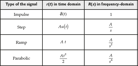
The standard test signals that can be applied to the control system are (i) impulse signal, (ii) step signal, (iii) ramp signal, (iv) parabolic signal and (v) sinusoidal signal.

However, to determine the time response characteristic of the control system, the first four of the above standard test signals are applied and to determine the frequency response characteristic, standard sinusoidal signal is applied.

5.3.1 Impulse Signal

The signal that is also called shock input, having its value as zero at all times except at is called impulse signal and it is shown in Fig. 5.1. This type of signal is not practically ­available since the occurrence of this type of signal is for a very small interval of time.

Fig. 5.1 ∣ Impulse signal

Mathematically, a unit-impulse signal is represented by

and .

From the above equations, it is clear that the area of the impulse function is unity. In ­addition, the area is confined to an infinitesimal interval on the t-axis and is concentrated only at .

Taking Laplace transform, we obtain .

When , the impulse signal becomes unit-impulse signal i.e., R(s) = 1.

The impulse response of a system with transfer function is given by

Taking inverse Laplace transform, we obtain ,

where is called “weighting function” of the system when unit-impulse signal is applied to the system.

The impulse signal is important due to the following reasons:

1. The impulse signal is very useful for analysing the system in time domain.
2. It is used to generate the system response if provided with the fundamental ­information about the system characteristic.
3. Transfer function of the system can be obtained once the impulse response of the system is known.
4. Impulse responses of the system can be obtained by taking the derivative of the step response of the system.
5. Depending on the area under the impulse response of the system, the stability of the system can be determined. For example, if the area under the impulse response curve is finite, then the system is stable with bounded input and bounded output.

5.3.2 Step Signal

The signal that resembles a sudden change by changing its value from one level (usually zero) to another level (may be A) in very small duration of time is known as step signal. The schematic representation of step signal is shown in Fig. 5.2.

Fig. 5.2 ∣ Step signal

The step signal is represented mathematically

(5.1)

The step signal can be obtained by integrating the impulse signal as given by

when , the step signal becomes unit-step signal .

Taking Laplace transform of Eqn. (5.1), we obtain

The step response of a system with transfer function is given by

Therefore,

Importance of Step Signal:

1. It represents an instantaneous change in the reference input signal of the system. For example, if the input is an angular position of a mechanical shaft, a step input represents the sudden rotation of the shaft.
2. It is useful in revealing the quickness of the system when an abrupt change is applied to the input.

5.3.3 Ramp Signal

The signal that depends linearly on the independent variable of the system, time t is known as ramp signal. The ramp signal that starts at zero resembles a constant velocity function. The schematic representation of ramp signal is shown in Fig. 5.3.

Fig 5.3 ∣ Ramp signal

The ramp signal is represented mathematically as

The unit-ramp signal can be obtained by integrating an unit-impulse signal twice or integrating a unit-step signal once, i.e.,

When , the ramp signal becomes unit-ramp signal.

i.e.,

Taking Laplace transform, we obtain

The ramp response of a system with transfer function is given by

Therefore,

Importance of Ramp Signal:

1. Ramp signal starts at time and varies linearly with it.
2. It helps in testing the response of the system when a ramp signal is applied to it. For example, if the input variable represents the angular displacement of the shaft, the ramp input denotes the constant speed rotation of the shaft.

5.3.4 Parabolic Signal

The signal that depends on the square of the independent variable of the system, time t is known as parabolic signal. The parabolic signal that starts at zero resembles a constant acceleration function. The schematic representation of parabolic signal is shown in Fig. 5.4.

Fig.5.4 ∣ Parabolic signal

The parabolic signal is mathematically represented as

Taking Laplace transform, we obtain

When , the parabolic signal is unit-parabolic signal. The parabolic signal can be obtained by integrating the ramp signal.

The parabolic response of a system with transfer function is given by

Therefore,

The different types of standard test signals with the corresponding r(t) in time-domain and R(s) in ­frequency-domain are given in Table 5.1.

Table 5.1 ∣ Standard test signals

Fig. E5.5

Solution:

Step Response

For the step response, the input excitation is .

Applying Kirchhoff's voltage law to the circuit shown in Fig. E5.5, we obtain

Taking Laplace transform, we obtain

Because of the presence of inductance , i.e., the current through an inductor cannot change instantaneously due to the conservation of flux linkages.

Therefore,

Hence,

Taking inverse Laplace transform, we obtain

Impulse Response:

For the impulse response, the input excitation is δ(t).

Applying Kirchhoff's voltage law to the circuit, we obtain

Taking Laplace transform, we obtain

Since i(0⁺) = 0,

Taking inverse Laplace transform, we obtain

Fig. E5.6

Solution:

Step Response

For the step response, the input signal x(t) = V₀u(t)

In the series RLC circuit shown in Fig. E5.6, the integro-differential equation is

or

Taking Laplace transform, we obtain

or

Due to the presence of inductor L, . Also, is the charge on the capacitor C at . If the capacitor is initially uncharged, then Substituting these two initial conditions, we obtain

Therefore,

where

Taking inverse Laplace transform, we obtain

Impulse Response

For the impulse response, the input signal .

Applying Kirchhoff's law to the circuit, we obtain

or

Taking Laplace transform, we obtain

or

Since and , we obtain

Taking inverse Laplace transform, we obtain

where and

Solution:

For the system given in Fig. E5.7, the input is and the output is and ­respectively.

Using D'Alemberts principle, we obtain

(1)

Fig.E5.7

For mass M,

(2)

Taking Laplace transform of Eqs. (1) and (2), we obtain

(3)

(4)

Representing Eqs. (3) and (4) in matrix form, we obtain

Using Cramer's rule, we obtain

Therefore,

i.e.,

Also,

Therefore,

Hence,

Therefore, the transfer functions of the given mechanical system are

and .

(i) For unit-step input:

When a unit-step signal is applied to the system, .

(ii) For unit-impulse input:

When a unit-impulse signal is applied to the system

Solution:

(i) For a unit-impulse input:

The transfer function of the system is given by . For a unit-impulse input, .

Hence,

Taking inverse Laplace transform, we obtain impulse response as

(ii) For a unit-step input:

The transfer function of the system is given by . For a unit-step input, .

Hence,

Using partial fractions, we obtain

Here,

Hence,

Taking inverse Laplace transform, we obtain step response as

(iii) For a unit-ramp input:

The transfer function of the system is given by .

For a unit-ramp input,

Hence,

Using partial fractions, we obtain

Here,

Hence,

Taking inverse Laplace transform, we obtain ramp response as

The unit-impulse, unit-step and unit-ramp responses of the given system are plotted and shown in Fig. E5.8.

Fig. E5. 8

Solution:

The closed-loop transfer function of the system is given by

For a unit-step input

Therefore,

Using partial fractions, we obtain

Here,

Therefore,

Taking inverse Laplace transform, we get a unit-step response as

Solution:

The closed-loop transfer function of the system is given by

For a unit-impulse Hence,

Taking inverse Laplace transform of the above equation, we obtain response of the ­system as

5.4 Poles, Zeros and System Response

Time response analysis of any system for standard test input signals can be obtained using inverse Laplace transform or differential equations. But these techniques are ­time-consuming and laborious. These issues can be overcome by employing pole-zero method. The system response can be ­determined in a short time by using pole-zero method.

5.4.1 Poles and Zeros of a Transfer Function

The transfer function of the system is expressed as

where a_n, a_n−1, …, a₀ and b_m, b_m−1, …, b₀ are constants.

The above transfer function can also be expressed as

where k is a real number. The constants , , … are called the zeros of , as they are the values of s at which becomes zero. Conversely, , , … are called the poles of , as they are the values of s at which becomes infinity.

The poles and zeros may be plotted in a complex plane diagram, referred to as the s-plane. In the complex s-plane where , a pole is denoted by a small cross and a zero by a small circle. This diagram gives a good indication of the degree of stability of a system.

For example, the pole-zero plot for the given transfer function

is plotted in Fig. 5.5.

For the given system, poles are and zeros are

Fig. 5.5 ∣ Poles and zeros of a system

5.4.2 Stability of the System

The stability of the system can be analysed based on the location of roots of the ­denominator polynomial or poles of the transfer function of the system. In addition, it does not depend on the input excitation applied to the system. The roots of the denominator polynomial or the poles of the transfer function of the system will determine whether the system is stable, unstable or marginally stable based on the location of poles in the s-plane, provided the degree of the denominator polynomial is greater than or equal to the degree of the ­numerator polynomial.

By finding the location of the poles, i.e., the roots of the denominator polynomial of the transfer function, the stability of the system can be determined.

1. For a stable system, all the poles of the transfer function must lie in the left half of the s-plane.
2. A system is said to be unstable, if any of the poles of transfer function are located in the right half of the s-plane.
3. A system is said to be marginally stable, if transfer function has any poles on the jω -axis in the s-plane provided the other poles of transfer function lie in the left half of the s-plane.

Although computer programmes are available for finding the roots of the denominator polynomial of order higher than three, it is difficult to find the range of a parameter for ­stability. In such cases, especially in control system design an analytical procedure called the Routh–Hurwitz stability criterion is used to analyse the stability of the system.

5.5 TYPE and ORDER of the System

The feed-forward transfer function of the system is and the system has a feedback transfer function .

5.5.1 TYPE of the System

Generally, the loop transfer function is expressed as

where are the coefficients that are constant and is the overall gain of the transfer function.

The TYPE of the system is decided based on the value n present in the general form of transfer function. The TYPE of the system and its corresponding general form of transfer function for some systems are given in Table 5.2.

Table 5.2 ∣ Type of the system and the corresponding general transfer function

5.5.2 ORDER of the System

For the system described earlier, the generalized closed-loop transfer function is given by

where K is the gain factor. The order of the system corresponds to the maximum power of s in the denominator polynomial.

Solution:

1. Since the number of poles at origin is 1, the transfer function is TYPE ONE system.
2. Since there is no pole at origin, the transfer function is TYPE ZERO system.
3. Since the number of poles at origin is 3, the transfer function is TYPE THREE system.
4. Since the number of poles at origin is 2, the transfer function is TYPE TWO system.

Solution:

1. Since the maximum power of in denominator polynomial is 3, the given transfer function is third-order system.
2. Since the maximum power of in denominator polynomial is 1, the given transfer function is first-order system.

5.6 First-Order System

The transfer function of the first-order system relating the input and output is given by

If no zeros exist in the system, the transfer function of the first-order system is given by

In the first-order system, the feed-forward transfer function of the system is and it has unity feedback system. Hence, the transfer function of the system is given by

where T is the time constant.

The block diagram of the first-order system is shown in Fig. 5.6.

Fig. 5.6 ∣ First-order system

5.6.1 Performance Parameters of First-Order System

1. (i) Rise Time : The time taken by the response of a system to reach 90% of the final value from 10% is known as the rise time . It can be obtained by equating the response of the system in time domain to 0.1 and 0.9 respectively. Hence, is given by

   

2. Delay Time : The time taken by the response of a system to reach 50 % of the final value is known as the delay time t_d. It can be obtained by equating the response of the system in time domain c(t) to 0.5.

   

3. Settling Time : The time taken by the response of a system to reach 98 % of the final value is known as the settling time. It can be obtained by equating the response of the system in time domain c(t) to 0.98. Hence, is given by

   

4. Steady-State Error : It is the measurement of a difference existing between the standard input signal applied and the output response obtained from the system c(t) when such standard signals are applied.

   

5.6.2 Time Response of a First-Order System

The time response of a first-order system when subjected to standard test signals such as unit-impulse, unit-step and unit-ramp inputs is discussed.

Time response of a first-order system subjected to unit-impulse input:

The transfer function of a first-order system is given by

Therefore,

For unit-impulse input, . Therefore,

Taking inverse Laplace transform, we obtain for

Time response of first-order system subjected to unit-step input:

We know that, for the first-order system

For unit-step input, and .

Substituting , we obtain

Using partial fractions, we obtain

Taking inverse Laplace transform, we obtain for

It is clear that the output value starts at zero and reaches unity as the independent variable time approaches infinity as shown in Fig. 5.7.

Fig. 5.7 ∣ Time response of first-order system subjected to step input

The steady-state error is given by

Also, the steady-state error of the system is determined using final value theorem as

Since , the first-order system is capable of responding to a unit-step input without any steady-state error.

Substituting in the time response of the system, we obtain

Here, the response of the system reaches 63.2% of the final value for the time constant T as shown in Fig. 5.7. The response of the system and the time constant of the system are inversely proportional to each other.

Time response of first-order system subjected to unit-ramp input:

We know that, for the first-order system,

For unit-ramp input or velocity input, ,

Therefore,

Using partial fractions, we obtain

Taking inverse Laplace transform, we obtain

The error signal is

The steady-state error is given by

Also, the steady-state error of the system is determined using final value theorem as

Thus, the first-order system under consideration will track a unit-ramp input with a steady-state error T, which is the time constant of the system.

The input signal, output signal and steady-state error for the first-order system ­subjected to ramp input are shown in Fig. 5.8.

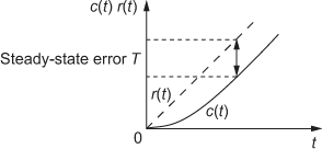
Fig. 5.8 ∣ Time response of first-order system subjected to ramp input

The time response of first-order system when subjected to various standard input signal is given in Table 5.3.

Table 5.3 ∣ Time response of first-order system subjected to various test signals

Time-domain specifications for a first-order system subjected to unit-impulse input:

The time response of the first-order system subjected to unit-impulse input is

The time-domain specifications are given below:

(i) Rise Time :

From the definition,

Hence, and are obtained as follows:

When the response of a system reaches 90 % of the final value, i.e., , the time is obtained as

When the response of a system reaches 10 % of the final value, i.e., , the time obtained as

Hence, rise time,

(ii) Delay Time :

From the definition,

When the response of a system reaches 50 % of the final value, i.e., , the delay time , is obtained as

Hence, delay time, sec.

(iii) Settling Time :

From the definition, for 2 % tolerance, the settling time is given by

When the response of a system reaches 98 % of the final value, i.e., , the time is obtained as

Hence, settling time, sec for 2 % tolerance

Similarly, for 5 % tolerance, the settling time,

Time-domain specifications for a first-order system subjected to unit-step input:

The time response of a first-order system subjected to unit-impulse input is

The time-domain specifications are given below:

(i) Rise Time :

From the definition,

Hence, and are obtained as follows.

When the response of a system reaches 90 % of the final value, i.e., , the time , obtained as

When the response of a system reaches 10 % of the final value, i.e., , the time obtained as

Hence, rise time,

(ii) Delay Time :

From the definition,

When the response of a system reaches 50 % of the final value, i.e., , the delay time obtained as

Hence, delay time, sec.

(iii) Settling Time :

From the definition, for 2 % tolerance, the settling time is given by

When the response of a system reaches 98 % of the final value, i.e., , the settling time obtained as

Hence, settling time, sec for 2% tolerance.

Similarly, for 5 % tolerance, the settling time,

5.7 Second-Order System

The transfer function of the second-order system is given by

If no zeros exist in the system, the transfer function of the second-order system is given by

For determining the time response and analysing the performance of the second-order system, let us assume that the feed-forward transfer function of the system is and it has a unity feedback. Hence, the transfer function of the second-order system is given by

where is an undamped natural frequency and is the damping ratio which is given by

The block diagram of the second-order system is shown in Fig. 5.9(a).

Fig. 5.9(a) ∣ Second-order system

5.7.1 Classification of Second-Order System

The second-order system can be classified into four types based on the roots of the characteristic equation of the system.

The characteristic equation of the second-order system is given by .

Its corresponding roots are given by

Here, the roots of the characteristic equation of the second-order system is dependent on the damping ratio .

The classification of the second-order system based on the roots of characteristic equation which depends on the damping ratio is given in Table 5.4.

Table 5.4 ∣ Classification of second-order system

5.7.2 Performance Parameters of Second-Order System

Delay Time : The time taken by the response of a system to reach 50 % of the final value is known as the delay time (t_d). It can be obtained by equating the response of the system to 0.5, given by

Rise Time : The time taken by the response of a system to reach 90 % of the final value from 10 % is known as the rise time. In addition, it can be defined as the difference between the time at which the response of the system has reached 10 % and 90 % of final value. The time at which response of the system reaches 10 % and 90 % can obtained by equating the response of the system to 0.1 and 0.9 respectively. Hence, is given by

Peak Time : The time taken by the response of a system to reach the first peak overshoot is known as the peak time. It can be obtained by differentiating the time response of the system and equating it to zero. i.e.,

Maximum Peak Overshoot : The maximum peak overshoot is obtained at the peak time of the response of a system, which is given by

where is the value obtained from the response of the system at peak time and is the steady-state value of the signal applied to the system.

The maximum peak overshoot is always represented as the percentage peak overshoot as

Special Case: If a standard unit signal is applied to a system, the steady-state value of the signal applied to the system will be 1 and hence the maximum peak overshoot will be

The relationship between the damping ratio of the second-order system and peak overshoot is shown in Fig. 5.9(b), irrespective of the input applied to the system. It is inferred that for an undamped system (), the peak overshoot is maximum; and for the critically damped system (), the peak overshoot is minimum. In addition, the peak overshoot does not exist for the second-order overdamped system (). Hence, peak overshoot varies only for the second order underdamped system ().

Fig. 5.9(b) ∣ Relation between peak overshoot and damping ratio

Settling Time : The time taken by the response of a system to reach 98% of the final value is known as the settling time. It can be obtained by equating the response of the system c(t) to 0.98.

Steady-State Error : It is the measurement of the difference existing between the standard input signal r(t) applied and the output response obtained from the system c(t) when such standard signals are applied.

5.7.3 Time Response of the Second-Order System

The time response of a second-order system (undamped, underdamped, critically damped and overdamped) when the system is subjected to standard test signals such as unit-step, unit-ramp and unit-impulse inputs is discussed in this section.

Time response of the second-order system subjected to unit-impulse input:

The closed-loop transfer function of the second-order system is

(5.1)

and its characteristic equation is given by

The roots of the equation are given by

For unit-impulse input and

Case 1: Undamped System

From Table 5.4, it is clear that for an undamped system,

Substituting in Eqn. (5.1), we obtain

The roots of its characteristic equation are given by

which are purely imaginary.

Substituting , we obtain

Taking inverse Laplace transform, we obtain the time response of the second-order un-damped system as

Case 2: Underdamped System

From Table 5.4, it is clear that for underdamped system,

For , the roots of the characteristic equation are

which are complex conjugate.

Here, and

Substituting in Eqn. (5.1), we obtain

Adding and subtracting to the denominator of the above equation, we obtain

Multiplying and dividing by , we obtain

Taking inverse Laplace transform, we obtain the response of an underdamped system as

Case 3: Critically Damped

From Table 5.4, it is clear that for critically damped system, .

For , the roots of the characteristic equation are given by

which are real and equal.

Substituting in Eqn. (5.1), we obtain

Substituting in the above equation, we obtain

Taking inverse Laplace transform, we obtain

The response of critically damped second-order system has no oscillations.

Case 4: Overdamped System

From Table 5.4, it is clear that for an overdamped system,

For , the roots of the characteristic equation are given by

which are real and unequal.

Substituting in Eqn. (5.1), we obtain

Assuming and , we obtain

Using partial fractions, we obtain

Taking inverse Laplace transform, we obtain the response of an overdamped system as

The input and output signals for the second-order system subjected to unit-impulse input are shown in Fig. 5.10.

Fig. 5.10 ∣ Responses of the second-order system subjected to impulse input for different cases

Time response of a second-order system subjected to a unit-step input:

The closed-loop transfer function of the second-order system is

and its characteristic equation is given by

The roots of the equation are given by

For unit-step input and .

Case 1: Undamped System

From Table 5.4, for an undamped system,

Substituting , we obtain

and the roots of its characteristic equation will be purely imaginary and it is given by

Substituting in Eqn. (5.1), we obtain

Using partial fractions, we obtain

Taking inverse Laplace transform, we obtain time response of the second-order undamped system as

Therefore, the response of an undamped second-order system when subjected to unit-step input is purely oscillatory which is shown in Fig. 5.11.

Fig. 5.11 ∣ Response of undamped second-order system subjected to unit-step input

Case 2: Underdamped System

From the Table 5.4, it is clear that for underdamped system, .

Substituting , the roots of the characteristic equation are given by

,

which are complex conjugates where and

Substituting in Eqn. (5.1), we obtain

Using partial fractions, we obtain

Adding and subtracting to the denominator of second term in the above equation, we obtain

Rearranging, we obtain

Hence,

where .

Multiplying and dividing by in the third term of the above equation, we obtain

Taking inverse Laplace transform, we obtain

Simplifying, we obtain

where

The response of an underdamped second-order system oscillates before settling to a final value is shown in Fig. 5.12. The oscillation depends on the damping ratio.

Fig. 5.12 ∣ Response of underdamped second-order system subjected to unit-step input

Case 3: Critically Damped System

From Table 5.4, it is clear that for critically damped system,

For , the roots of the characteristic equation are given by

which are real and equal.

Substituting in Eqn. (5.1), we obtain

Since ,

Using partial fraction expansion, we obtain

Taking inverse Laplace transform, we obtain

The response of a critically damped second-order system has no oscillations as shown in Fig. 5.13.

Fig. 5.13 ∣ Response of a critically damped second-order system subjected to unit-step input

Case 4: Overdamped System

From Table 5.4, it is clear that for underdamped system,

For , the roots of the characteristic equation are given by

which are real and unequal.

Substituting in Eqn. (5.1), we obtain

Using partial fractions, we obtain

Therefore,

Taking inverse Laplace transform, we get the response of the overdamped system as

Therefore, the response of an overdamped second-order system when subjected to unit-step input has no oscillations but it takes longer time to reach the final steady value as shown in Fig. 5.14.

Fig. 5.14 ∣ Response of an overdamped second-order system when subjected to unit-step input

The responses of the second-order system when subjected to a unit-step input are shown in Fig. 5.15.

Fig. 5.15 ∣ Responses of different second-order systems when the system is excited by unit-step input

Time response of a second-order system subjected to a unit-ramp input

The closed-loop transfer function of the second-order system is

and its characteristic equation is given by

The roots of the equation are given by

For a unit-impulse input, and

Case 1: Undamped System

From Table 5.4, it is clear that for an undamped system,

Substituting in Eqn. (5.1), we obtain

and the roots of its characteristic equation will be purely imaginary as given by

Substituting in Eqn.(5.1), we obtain

Using partial fractions, we obtain

Taking inverse Laplace transform, we obtain the time response of the second-order undamped system as

Case 2: Underdamped System

From Table 5.4, it is clear that for an underdamped system, .

For , the roots of the characteristic equation are given by which are complex conjugate.

Substituting in Eqn. (5.1), we obtain

Using partial fractions, we obtain

Taking inverse Laplace transform, we obtain the time response of an underdamped system as

Case 3: Critically Damped System

From Table 5.4, it is clear that for critically damped system,

For , the roots of the characteristic equation are given by which are real and equal.

Substituting in Eqn. (5.1), we obtain

Substituting in above equation, we obtain

Using partial fractions, we obtain

Taking inverse Laplace transform, we obtain

Case 4: Overdamped System

From Table 5.4, it is clear that for underdamped system,

For , the roots of the characteristic equation are given by which are real and unequal.

Substituting in Eqn. (5.1), we obtain

Using partial fractions, we obtain

Taking inverse Laplace transform, we obtain the time response of the overdamped system as

where .

5.7.4 Time-Domain Specifications for an Underdamped Second-Order System

The time-domain specifications of an underdamped second-order system when subjected to different standard signals are discussed below.

Underdamped second-order system subjected to a unit-impulse input:

The time response of an underdamped second-order system is given by

where

Peak Time :

The peak time,

where .

Maximum Peak Overshoot :

The maximum peak overshoot when a standard unit signal is applied, is given by

Substituting the peak time in the above equation, we obtain

Using the right angled triangle shown in Fig. 5.16, we obtain

Also, the percentage peak overshoot is given by

Settling Time :

For 2 % of tolerance, the settling time is given by

For determining the settling time, the oscillatory component present in the response of the system is eliminated. Only the exponential component is considered because as time t tends to infinity, the response of the system tries to follow the input.

Hence, the modified time response of the system is given by

Settling time for 2 % of tolerance is determined as

Solving the above equation, we obtain

Similarly, we can solve for 5% of tolerance and its settling time is

sec

Underdamped second-order system subjected to a unit-step input:

The time response of an underdamped second-order system is given by

where .

Rise Time :

From the definition,

But for an underdamped second-order system,

Using the above equation, the response of the second-order system,

For n = 1,

sec.

Peak Time :

From the definition,

Equating the above equation to zero, the peak time can be determined:

Simplifying, we obtain

Using the term , a right-angled triangle can be formed as shown in Fig. 5.16. The termsand can be replaced by and respectively.

Fig. 5.16 ∣ Right angled triangle for damping ratio

Rewriting the above equation, we obtain

Using the formula , we obtain

or

We know that the peak time is the time taken by the response to reach the first peak overshoot. Therefore,

sec.

The peak time given by the above equation corresponds to one-half cycle of the frequency of damped oscillations.

Maximum Peak Overshoot :

From the definition, the maximum peak overshoot when a standard unit-step signal is applied is given by

Substituting the peak time in the above equation, we obtain

Using the formula and using the right-angled triangle i.e., shown in Fig. 5.16, we obtain

Also, the percentage peak overshoot is given by

%

Settling Time :

For 2 % of tolerance, the settling time is given by

For determining the settling time, the oscillatory component present in the response of the system is eliminated and only exponential component is considered because as time t tends to infinity, the response of the system tries to follow the input.

Hence, the modified time response of the system is given by

Settling time for 2 % of tolerance is determined as

Solving the above equation, we obtain

Similarly, the settling time for 5 % of tolerance is given by

Steady-State Error:

The steady-state error is given by

Hence, the second-order underdamped system has zero steady-state error.

Solution:

The characteristic equation is

Comparing the above equation with the standard form , we obtain

and

Since the given system is underdamped.

Fig. E5.14

Solution:

Let us assume that

is the number of teeth of the gear in the motor side.

is the number of teeth in the load side.

= is the gear ratio.

is the load torque in Newton-metre.

is the forward loop gain in Newton-metre/rad error.

is the moment of inertia in kg-m².

is the friction coefficient in Newton metre/rad/sec.

is the moment of inertia of the load.

is friction coefficient of the load.

T(s) = is the load torque referred to the motor shaft.

is the friction coefficient at the motor shaft and

J = is the moment of inertia at the motor shaft.

If is the error signal, the actuating signal to drive the motor and the load is . If the system is a second-order system, then the differential equation of the system is

which is referred to the motor shaft.

Equating the above equation to the actuating signal , we obtain

Taking Laplace transform on both the sides, we obtain

(1)

But

Substituting the error signal in Eqn. (1), we obtain

(neglecting load torque)

Therefore, the transfer function of the system is

,

Comparing the above equation with standard closed-loop transfer function of the second-order system , we obtain

and

Therefore,

Also, using the above relations, we obtain .

Determination of steady-state error:

1. For unit-step input:

   Substituting in Eqn. (1), we obtain

   

   Solving the above equation, we obtain

   

   For unit-step input, we have

   Hence,

   Therefore, the steady-state error of the system is

   

   But when T is neglected,

2. For a ramp input with slope

   

Solution:

The formulae for and for the servo system are

Substituting the known values in the above equations, we obtain

Fig. E5.16

Solution:

Input velocity,

Motor constant,

The formulae for and for the servo system are

Substituting the known values in the above equations, we obtain

and at the motor shaft.

Gain of the amplifier

Steady-state error at motor shaft .

Fig. E5.17

Solution:

Referring to the load side, the moment of inertia at the load shaft is

The total friction at the load shaft

Therefore,

Steady-state error,

If is the loop gain measured at the load side (feedback is given from the gear), then

But

Therefore,

Solution:

The closed-loop transfer function can be rearranged as

Comparing the above equation with standard closed-loop transfer function of the second-order system , we obtain

i.e., (1)

and i.e., (2)

Given the maximum overshoot = 6 % = 0.06

Therefore,

Taking natural logarithm on both sides, we obtain

Solving the above equation, we obtain (3)

Also, given the time for peak overshoot

Therefore,

Solving the above equation, we obtain

(4)

For a step input of 10 Nm applied to the system,

Therefore,

The K can be obtained by determining the steady-state error of the system. It is obtained by using final value theorem.

Steady-state error

(5)

Therefore,

Using Eqn. (1) and Eqn. (4), we obtain

Similarly, substituting the known values in Eqn. (2), we obtain

Therefore, the overall transfer function of the given system is

Fig.E5.19

Solution:

The output voltage across the capacitor is

Applying Kirchhoff's voltage law, we obtain

Taking Laplace transform of the above equations, we obtain

(1)

and

Simplifying, we obtain

(2)

Substituting Eqn. (2) in Eqn. (1), we obtain

Hence, the transfer function for the system is obtained by

Comparing the above equation with standard closed-loop transfer function of the second-order system , we obtain

and

Therefore, and

Fig.E5.20

Solution:

We know that, for the given system, the damped natural frequency and damping ratio are

and

Substituting the known values, we obtain

and

The time-domain specifications are

and

Solution:

The closed-loop transfer function of the system is given by

Comparing the above equation with standard closed-loop transfer function of the second-order system, we obtain

, , .

Hence, the time-domain specifications are obtained as

Peak time,

Rise time,

Percentage peak overshoot,

Settling time for 2 % of tolerance,

and for 5 % of tolerance,

Solution:

The closed-loop transfer function of the system is given by

Comparing the above equation with standard closed-loop transfer function of the second-order system, we obtain

and

Hence, the time-domain specifications of the system subjected to unit-step input are obtained as

Rise time,

Percentage peak overshoot,

Peak time, .

Time delay, sec.

Settling time, .

Solution:

Given

Taking Laplace transform on both the sides of the given differential equation, we obtain

Therefore, the transfer function of the system can be obtained as

Comparing the above equation with standard closed-loop transfer function of the second-order system, we obtain

ω²_n = 25, i.e., ω_n = 5 and 2ξω_n = 8 i.e., ξ = 0.8

Therefore,

Since for the given second-order system, the damping ratio is , the system is an underdamped system. Hence, the response for the second-order underdamped system when a unit-step signal applied is given by

But in this system, as the transfer function is multiplied by two, the response must also be multiplied by two.

Therefore, by substituting the known values in the above equation, we obtain

The above equation is the response of the system subjected to a unit-step input. Hence, when the system is subjected to a step input of magnitude 2.5 units, we obtain the response of the system as

The response of the system will be at its maximum value at

Therefore,

Therefore, the maximum output is obtained as

Solution:

The closed-loop transfer function of the system is given by

Comparing the above equation with the standard form, we obtain

, and

Hence, the value must be changed from 0.0911 to 0.4037 to reduce the percentage peak overshoot from 75 % to 25 %.

Hence, by taking the ratio for different values of , we obtain

where K is the gain for and K₁ is the gain for

Hence, the gain K must be multiplied by 0.05092 to change percentage peak overshoot from 75% to 25%.

Solution:

The closed-loop transfer function of the system is given by

Comparing the above equation with the standard form, we obtain

,i.e., and

Case (i):

Consider the time constant T to be constant. Let K = K₁ for and K = K₂ for .

Using the formulae for and taking the ratio, we obtain

Solving the above equation, we obtain

Hence, the gain K has to be multiplied by the factor 0.09 to reduce the damping ratio from 0.5 to 0.15.

Case (ii):

Consider the gain K to be constant. Let T = T₁ for and T = T₂ for .

Using the formula for and taking the ratio, we obtain

Solving the above equation, we obtain

Hence, the time constant T has to be multiplied by the factor 4 to reduce the damping ratio from 0.8 to 0.4.

Solution:

The Laplace transform of a unit-step signal applied to the system is given by

Taking Laplace transform of the time response of the system c(t), we obtain

Hence, the closed-loop transfer function is

Comparing the above equation with the standard form, we obtain

 i.e., rad/sec

and  i.e.,

Since the damping ratio of the system , the system is overdamped.

Fig. E5.27

Solution:

For the given system, the closed-loop transfer function of the system is given by

Comparing the above equation with the standard form, we obtain

i.e., and i.e.,

Also,

The response of the second-order underdamped system is given by

Substituting the known values in the above equation, we obtain

Fig. E5.28

Solution:

Using Newton's second law to the above system, we obtain

Taking Laplace transform and using the given values, we obtain

Comparing the above equation with the standard form, we obtain

i.e.,

and i.e.,

Damped natural frequency

For a second-order underdamped system, the step response of the system is given by

The given transfer function is modified as given in Eqn.(5.1) as

Then, the response of the system is given by

where

Hence,

Fig. E5.29

Solution:

Fig. E5.30

Solution:

Using Newton's second law to the mass M, we obtain

Taking Laplace transform, we obtain

Comparing the above equation with the standard form, we obtain

and

Hence, undamped natural frequency,

Damping factor,

Damped natural frequency,

Solution:

For the given system, the closed-loop transfer function of the system is given by

Comparing the above equation with the standard form, we obtain

i.e., and i.e.,

For the given damping ratio

Hence, undamped natural frequency,

Damped natural frequency,

Settling time,

Percentage peak overshoot,

Peak time,

Solution:

Given

Taking Laplace transform, we obtain

Comparing the above equation with the standard form , we obtain

i.e., and i.e.,

Hence, undamped natural frequency, rad/sec.

Damping ratio,

Damped natural frequency, rad/sec, rad

The time-domain specifications are

Delay time,

Rise time,

Peak time,

Settling time,

% peak overshoot,

Thus, the output response of the second-order system subjected to unit-step signal is given by

where

Substituting the known values, we obtain

Fig. E5.33(a)

Solution: From Fig. E5.33(a),

After successive reduction, the block diagram is shown as

Fig. E5.33(b)

From Fig. E5.33(b), the following closed-loop transfer function is obtained:

The standard second-order transfer function is given by

Comparing the above equations, we obtain

and

Substituting we obtain

and

For 25% overshoot, the equation is written as

Taking natural logarithm on both the sides, we obtain

Solving for we obtain

Also,

Solving the above equation for we obtain

Therefore,

and

Fig. E5.34

Solution: The closed-loop transfer function for the given system is given by

Comparing the above equation with the standard form, we obtain

i.e.,

and i.e.,

Here, undamped natural frequency,

Given rad/sec. Hence, .

Given ξ = 0.7.

The damping ratio,

i.e.,

Therefore, a = 0.225.

Solution: The closed-loop transfer function of the second-order system is given by

Comparing the above equation with the standard form, we obtain

and

Hence, undamped natural frequency,

Damping ratio,

Damped natural frequency, rad/sec

The time-domain specifications are obtained as

Rise time,

Peak time,

% maximum peak overshoot,

Settling time,

When the second-order system is subjected to a unit-step input, the output response is obtained as

Substituting the known values in the above equation, we obtain

.

Solution: Given the open-loop transfer function of the given system is

The system has a unity feedback,

Hence, the closed-loop transfer function of the system is given by

Comparing the above equation with the standard form, we obtain

and

Hence, undamped natural frequency rad/sec.

Damping ratio,

Damped natural frequency, rad/sec.

rad.

It is important to note that the formula for determining the time-domain specifications except for % peak overshoot of the given second-order system is same irrespective of the magnitude of the input signal applied to the system.

Hence, the time-domain specifications for the given system are obtained as

Rise time,

Peak time,

% percentage peak overshoot,

Fig. E5.37

Solution: The closed-loop transfer function of the system is

The characteristic equation of the system is

Comparing the above equation with the standard form , we obtain

and

Therefore, ,

and

Using peak time and maximum peak overshoot formula, we obtain

and

Solving the above equation, we obtain

and

Solution: For the given closed-loop servo system, we obtain

Substituting the known values, we obtain

Therefore, % overshoot = = = 30.09%

To find settling time for 5% oscillation

It is known that

e^-m × 100 = 5 and

Therefore,

and the time constant,

Hence,

Solution: The closed-loop transfer function of a unity feedback system is

Comparing the above equation with the standard form, we obtain

The maximum overshoot is given by

For an input of 20°, the overshoot =

The time at which the maximum overshoot occurs is

Rise time,

where

Hence,

For 6 % error

Time constant,

Settling time,

5.8 Steady-State Error

The objective of the control system is to make the system response follow the specific ­standard reference signal applied to the system in a steady state without any deviation. The steady state occurs due to the presence of non-linearities in the system. The accuracy of the control system is measured by steady-state error. The steady-state error is defined as the difference between the output response of the control system and the standard ­reference signal applied to it. The occurrence of steady-state error in the control system is almost inevitable. But the steady-state error can be maintained at a minimum value by satisfying the specifications of the transient response of the system.

5.8.1 Characteristic of Steady-State Error

For the system shown in Fig. 5.17(a), is the step input, is the output and is the error. As equals in the steady-state condition, there will be no error existing in the system (i.e., = 0) which is practically impossible with the pure gain K. Thus, in the steady-state condition, the relation between the steady-state value of the error and the steady-state value of the output is given by . Thus, for achieving a smaller steady-state value of the error , a large value of gain K is used. Hence, a steady-state error will be present in the system if a step input is applied to the system that has a gain in the forward path.

Fig 5.17 ∣ A simple closed-loop system

When a step input is applied, the steady error of the system becomes zero if the gain of the system is replaced by an integrator as shown in Fig. 5.17(b). Thus, the steady-state error varies with the gain value associated with the system.

5.8.2 Determination of Steady-State Error

The steady-state error of a system when different types of standard test input signals are applied to it is discussed in this section. The steady-state error can be determined for the system with unity feedback and also for the system with non-unity feedback in terms of closed-loop transfer function of the system.

5.8.3 Steady-State Error in Terms of G(s)

In this section, we will be determining the steady-state error of the system with unity ­feedback path. Let be the transfer function of the forward path and . Although, the steady-state error is calculated in terms of closed-loop transfer function of the system for a unity feedback system, it is better to use the open-loop transfer function .

Fig 5.18 ∣ A simple closed-loop system with unity feedback

Consider a system with unity feedback as shown in Fig. 5.18. The error is the ­difference between the input and the output . Thus, by solving for , it is­ ­possible to get an expression for the error.

Therefore,

Solving the above equations, we obtain

Applying the final value theorem to above the equation, we get the steady-state error of the system as

Thus, the steady-state error can be determined for different standard test input signals and systems . Let us consider the system with forward path transfer function as and we can determine the relationship between the steady-state error and by applying some standard signals such as unit-step input, unit-ramp input and unit-parabolic input.

Step Input

For a unit-step signal, ,

Case 1: if at least one pole exists at the origin, i.e.,

The steady-state error,

Case 2: if there does not exist a pole at origin, i.e., n = 0

which is finite and yields a finite steady-state error.

Ramp Input

For a unit-ramp signal, ,

Case 1: If there are two or more poles at the origin, i.e., .

The steady-state error

Case 2: If there is only one pole at the origin, i.e.,

which is finite and leads to constant steady-state error

Case 3: If there is no pole at the origin,

which leads to an infinite steady-state error.

Parabolic Input:

For a unit-parabolic signal, ,

Case 1: If there are three or more poles at the origin, i.e.,

The steady-state error will be zero i.e., .

Case 2: If there are two poles at the origin, i.e.,

The steady-state error will be constant finite value.

Case 3: If there is less than one pole at the origin, i.e.,

The steady-state error will be infinite, .

5.8.4 Steady-State Error in Terms of T(s)

Let be the transfer function of the forward path and be the transfer function of the feedback path. In this case, the steady-state error is calculated in terms of closed-loop transfer function of the system .

Fig 5.19 ∣ A simple closed-loop system

Referring to Fig. 5.19, the error is the difference between the input and the output . Thus, by solving for , it is possible to get an expression for the error. Then, by applying final value theorem, the steady-state error is obtained as

where

Therefore,

Applying the final value theorem, we obtain steady-state error of the system as

5.8.5 Static Error Constants and System Type

In general, the response of a system consists of transient response and steady-state response. In the previous sections, we have discussed about the transient response of the system and its performance specifications such as damping ratio, natural frequency, settling time and percent overshoot subjected to different standard signals. ­Similarly, the ­performance specifications of steady-state error called static error constants can be ­determined as given below.

Static Error Constants

For a step input, its corresponding steady-state error is

For a ramp input, its corresponding steady-state error is

For a parabolic input, its corresponding steady-state error is

are collectively known as static error constants and they are separately termed as position error constant, velocity error constant and acceleration error constant respectively.

Position error constant,

Velocity error constant,

Acceleration error constant,

Since the static error constants are present at the denominator of the steady-state error equation, the steady-state error will decrease as the static error constant increases. It is clear that the above three static error constants are dependent on the transfer function of the system and the number of poles present at the origin. But it is known that the number of poles present at the origin determines the TYPE of the system. Hence, the relationship among the TYPE of the system, static error constant and steady-state error of the system are given in Table 5.5.

Table 5.5 ∣ Relationship among the input, system type, static error constant and steady-state error

The significant features of static error constants:

1. Steady-state error characteristics are specified using static error constants.
2. The TYPE of the system, the type of input applied to the system can be determined by knowing the static error constants.
3. These coefficients are used for error analysis only if the input is step, ramp and parabolic inputs.
4. The values of static error constants given in Table 5.5 are for the systems only with unity feedback.
5. If the input applied to a system is a linear combination of the inputs (step, ramp and parabolic), then the steady-state error can be obtained by superimposing the errors obtained due to each input.

Solution: The characteristic equation of the system is

Therefore, the steady-state error of the system is

Steady-state error for different inputs:

1. For step input ,

   Therefore,

2. For ramp input ,

   

3. For acceleration input ,

   

Solution: The characteristic equation of the system,

Comparing the above equation with the standard form , we obtain

Substituting known values, we obtain

Also,

Hence,

Steady-state error for the ramp input:

Velocity error constant

Therefore,

Fig. E5.42(a)

Solution: The equivalent block diagram of the system is shown in Fig. E5.42(b).

Fig. E5.42(b)

Input velocity,

Motor constant

We know that, for the given system and

Therefore,

=

Gain of the amplifier =

Steady-state error at motor shaft,

Solution:

Fig. E5.43

Speed = 1000 km/hr

Therefore, the distance travelled by the target for 1 sec = 277 m

From Fig. E5.43, we obtain

Therefore,

But we know that for a ramp input, the steady-state error is obtained as

Therefore, for the given system where the input R is an angle , we obtain

Therefore, the ramp error constant,

Solution:

Given the open-loop transfer function .

Position error constant,

Velocity error constant,

Acceleration error constant,

Hence, the steady-state error for

1. the input is given by
2. the input is given by
3. the input is given by

Hence, the total steady-state error is given by

.

Solution: (i) Given the open-loop transfer function .

1. Position error constant,
2. Velocity error constant,
3. Acceleration error constant,

(ii) The steady-state error for ramp input is given by

Give the magnitude of ramp input, A = 4

Therefore,

Solution: Given the open-loop transfer function .

1. Position error constant,
2. Velocity error constant,
3. Acceleration error constant,

Hence, the steady-state error for

1. the input 3 is given by
2. the input is given by
3. the input t² is given by

Hence, the total steady-state error is given by

Fig. E5.47

Solution: Given and input is step of 1,000

The input

For step input,

Therefore, steady-state error,

where A = magnitude of step input.

i.e.,

Therefore, the steady-state temperature can be determined as

Hence, .

Solution: Since there exist no poles at the origin, the system is TYPE 0 system.

From Table 5.5, the unit-step input gives a constant steady-state error for TYPE 0 system.

Therefore,

Position error constant,

and the steady-state error,

Solution:

Given the open-loop transfer function and

Position error constant,

Velocity error constant,

Acceleration error constant,

Hence, the steady-state error for

1. the input 1 is given by
2. the input is given by
3. the input 9t² is given by

Hence, the total steady-state error is given by

Given the steady-state error of the system Therefore,

Hence, K = 90.

Solution:

Given the open-loop transfer function and

Position error constant,

Velocity error constant,

Therefore, the steady-state error for

1. the input is given by
2. the input is given by

Hence, the total steady-state error is given by

Given the steady-state error of the system is 0.1. Therefore,

Therefore, K1 = 60.

Fig. E5.51

Solution:

We have

or

The characteristic equation is

or

or

Comparing with , we obtain

or .

Solution:

Given the open-loop transfer function

Position error constant,

Velocity error constant,

Acceleration error constant,

The steady-state error of the system subjected to parabolic input is given by

5.8.6 Generalized or Dynamic Error Coefficients

The error coefficients discussed in the previous sections are known as static error coefficients since each of the input applied to the system to get the steady-state error is not time-varying quantity. Also, it is impossible to design such control systems to maintain zero ­steady-state error when the input applied is a time-varying quantity. The steady-state error of such ­systems is determined as follows:

The error of a unity feedback control system as discussed in the static error ­coefficients is given by

The error transfer function, can be expressed as

where, in general, the coefficients , , , , … are defined as dynamic error ­coefficients or generalized error coefficients.

The generalized error coefficients are obtained using the formula

(5.2)

To determine the steady-state error using the generalized or dynamic error coefficients, the following steps are followed:

Taking inverse Laplace transform, we obtain

Therefore, the steady-state error is given by

The relationship between the static and dynamic (generalized) error coefficients are given below which are not difficult to prove.

, and

Solution: The transfer function of the system relating the error and the input of the system is given by

Also, the error series of the system is given by

Here, the coefficients , , , , … are obtained using the formula

1. For input

   From the given input, we obtain

   Therefore, steady-state error

   Hence,

   And,

2. For the input

   From the given input, we obtain

   and other differentials as zero.

   Therefore,

   Hence,

   and,

3. For the input

   From the given input, we obtain

   , and other higher differentials are zero.

   Therefore,

   where

   Hence,

4. For the input

   From the given input, we obtain

   ,

   Therefore,

   

   Substituting the known values in the given equation, we obtain

   

   

   

Fig. E5.54

Solution: From the block diagram shown in Fig. E5.54, we obtain

For the negative feedback system with , the function is

For the given input , we have

and

Therefore, the steady-state error is given by

Therefore, the generalized error coefficients are

Hence, the steady-state error of the system is

.

Solution: The error transfer function for the system is given by

Dividing the numerator by denominator directly, we obtain

But the error transfer function is given by

Using the above two equations, we obtain

Taking inverse Laplace transform, we obtain

From the given input , we obtain

Hence, the steady-state error of the system is

Solution: The open-loop transfer function of a unity feedback system is given by

Therefore, the error transfer function of the system is given by

The generalized error coefficients for the given system are determined using Eqn. (5.2) as

Therefore,

Thus,

Therefore, the generalized error coefficients are

Thus, the error series of the system using the generalized error coefficients is

Solution: Given

Therefore,

Hence, the static error constants are

To determine :

For the input , we obtain

Error signal in s-domain,

Therefore, steady-state error

5.9 Effect of Adding Poles and Zeros in the Second-Order System

Consider a second-order system with the open-loop transfer function as and unity feedback. The closed-loop transfer function of the system is obtained as . The time-domain specifications of the second-order system are rise time, peak time, peak overshoot, settling time, etc. These time-domain specifications can be modified (either be increased or decreased) by adding either a pole or a zero.

5.9.1 Effect of Adding Poles

If a pole is added to the above-mentioned system, the closed-loop transfer function of the system will be modified as . Assuming a fixed value for and varying , the response of the system can be determined. Fig. 5.20 shows the response of the second-order system subjected to a unit-step input by varying the pole .

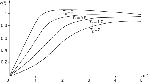
Fig. 5.20 ∣ Step response of the second-order system for different pole location

The following changes occur by adding pole to the existing system:

1. Peak overshoot decreases as decreases.
2. Number of oscillations existing in the system becomes less as decreases.
3. Increase in rise time.
4. System becomes more sluggish as decreases.

Also, it is important to know the fact that by adding pole to the system in the forward path, the system will have the opposite effect.

5.9.2 Effect of Adding Zeros

If a zero is added to the above-mentioned system, the closed-loop transfer function of the system will be modified as . Assuming a fixed value for and varying , the response of the system can be determined. Fig. 5.21 shows the response of the second-order system subjected to a unit-step input by varying the zero .

Fig. 5.21 ∣ Step response of the second-order system for different zero location

The following changes occur by adding pole to the existing system:

1. Increases rise time as increases.
2. Increases peak overshoot and number of oscillations as increases.

5.10 Response with P, PI and PID Controllers

The transient response specifications and steady-state response specifications of the ­system are to be maintained at a specific value for maintaining the system stability. Among the ­different transient response specifications discussed earlier in this chapter, the value of ­maximum overshoot is taken as the criteria to maintain stability and for steady-state response, steady-state error is taken as the criteria. The controllers are used to maintain those specifications at a specific value instead of zero or infinity. Here, a general second-order system is used and different types of controllers are used to maintain the steady-state error at a specific value. The output signal of the controller or the input signal of the system is known as actuating signal.

5.10.1 Proportional Derivative Control

The derivative controller alone is not used in the control system due to some reasons. One of the reasons is that if there is a constant steady-state error in the system, the derivative ­controller does not take any corrective measure since the derivative of a constant value is zero, which makes the error to prevail in the system even though a derivative controller is used. Hence, the derivative controller is used alongwith some of the other controllers.

The block diagram of the system with proportional derivative controller with unity ­feedback system is shown in Fig. 5.22. The system is a general second-order system. The ­actuating ­signal of the controller consists of the sum of the control action given by the ­proportional derivative controller. Hence, the actuating signal is given by

Taking Laplace transform, we obtain

Fig. 5.22 ∣ Proportional derivative controller of second-order system

The closed-loop transfer function of the system using proportional derivative control is given by

Comparing the above equation with the standard form , we obtain

where is the damping ratio of the system with the controller.

From the above equation, it is clear that effective damping ratio has been increased by using the controller, thereby reducing the maximum overshoot.

The forward path transfer function of the system shown in Fig. 5.22 is given by

and the feedback path transfer function is

Hence, the error function is given by

For a unit-ramp input,

Therefore,

Therefore,

The steady-state error for unit-ramp input is given by

It is clear that by introducing the proportional derivative controller in the system, the damping ratio has been increased without changing the TYPE of the system and ­undamped natural frequency of the system. Also, due to the increase in the damping ratio of the system, the maximum peak overshoot and settling time that have direct impact on have been reduced. Also, the steady-state error of the system remains unchanged even though a proportional derivative controller has been used.

5.10.2 Proportional Integral Control

The block diagram of a unity feedback system with proportional integral controller is shown in Fig. 5.23. The system is a general second-order system. The actuating signal of the controller consists of sum of the control action given by the proportional and integral controllers. Hence, the actuating signal is given by

where is a constant.

Taking Laplace transform, we obtain

Fig. 5.23 ∣ Proportional integral controller of second-order system

The closed-loop transfer function of the control system is given by

The characteristic equation of the system with integral control is given by

The order of the system has been increased due to the inclusion of integral controller in the existing second-order system.

The forward path transfer function of the system shown in Fig. 5.23 is given by

and the feedback path transfer function,

Hence, the error function is given by

For a unit-ramp input , 

Hence,

The steady-state error is given by

For unit-parabolic input,

The steady-state error is given by

It is clear that by introducing proportional integral controller in the system, the type and order of the system can been increased. Also, the steady-state error of the system by ­introducing proportional integral controller in the system has been decreased for certain types of inputs such as parabolic input.

5.10.3 Proportional Plus Integral Plus Derivative Control (PID Control)

The block diagram of a unity feedback system with proportional integral derivative controller is shown in Fig. 5.24. The system is a general second-order system. The actuating signal of the controller consists of sum of the control action given by the proportional, integral and derivative controllers. Hence, the actuating signal is given by

Fig. 5.24 ∣ Proportional integral derivative controller of second-order system

The actuating signal for the PID control is given by

Taking Laplace transform, we obtain

From the above sections, we come to know that proportional derivative controller improves the transient response specifications (peak overshoot, settling time) and proportional integral controller improves the steady-state response specifications (steady-state error), but the proportional integral derivative controller that combines the actions of above-mentioned controllers helps in improving both the transient and steady-state response specifications.

Fig. E5.58

Solution:

Fig. E5.59

Solution: The closed-loop transfer function of the system is given by

Comparing the above equation with the standard form , we obtain

, and .

Since the damping ratio of the system with derivative control is given as 1 (For critically damped system) substituting 1 in the above equation we obtain

Hence, settling time is given by

5.11 Performance Indices

The qualitative measure of the performance of a system is very important in designing a control system. Performance index is a qualitative measure of the performance of the system where certain parameters of the system can be varied for getting the optimum design and hence emphasizing on system specifications. A particular performance index referred as cost function should be chosen and has to be measured for obtaining the optimal design. There are many cost functions of which some are discussed below:

1. Integral of the absolute magnitude of the error (IAE)

   

   where error

   The integral value is minimum for a damping factor of 0.7 for a second-order system.

2. Integral of the square of the error (ISE)

   

   The integral value is minimum for a damping factor of 0.5 for a second-order system.

3. Integral of time multiplied by the absolute value of error (ITAE), which is given by

   

   The integral value is minimum for a damping factor of 0.7 for a second-order system.

4. Integral of time multiplied by the squared error (ITSE)

   ITSE

5. Integral of squared time multiplied by the absolute value of error square (ISTAE)

   ISTAE

6. Integral of squared time multiplied by square error (ISTSE)

   ISTSE

The last three performance indices are not used due to the difficulty existing in ­determining the values. Figure. 5.25 shows the performance indices of the system obtained using the response .

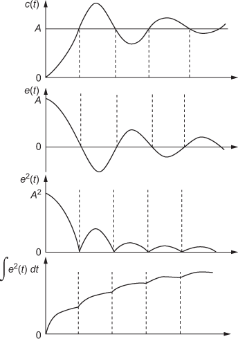
Fig. 5.25 ∣ Performance indices obtained using the response of the system

Review Questions

1. What do you mean by time response of a system and what are its components?
2. Define transient response system and steady-state response of a system. In addition, mention the significance of these responses of the system.
3. Define the standard tests signals used for time-domain studies:

   (a) Impulse signal and unit-impulse signal, (b) step signal and unit-step signal, (c) ramp signal and unit-ramp signal and (d) parabolic signal.

4. What is the importance of impulse signal, step signal, ramp signal and parabolic ­signal?
5. What is the relation existing between the standard test signals?
6. Define the type and the order of a system.
7. What do you mean by first- and second-order systems? Give examples.
8. List out the performance indices used for evaluating the performance of first-order system.
9. Derive the response of a first-order system subjected to the following:

   (a) Impulse input and unit-impulse input, (b) step input and unit-step input and (c) ramp input and unit-ramp input.

10. Derive the performance indices of a first-order system when the system is excited by the following inputs: (a) Unit-impulse, (b) step input and (c) ramp input.
11. By deriving the unit-step response of a first-order system, obtain the response of the system when it is excited by (a) unit-impulse input and (b) unit-ramp input.
12. Sketch the responses of a first-order system subjected to a (a) unit-impulse input, (b) unit-step input and (c) unit-ramp input.
13. How is second-order system classified based on the damping ratio ?
14. What are the effects of damping ratio on the response of a second-order system?
15. List out the performance indices used for evaluating the performance of a second-order system.
16. Define the following performance indices and give its expression:

    (a) Delay time, (b) rise time, (c) peak time, (d) maximum peak overshoot and (e) ­settling time.

17. Discuss the relationship between the maximum peak overshoot and damping ratio.
18. Derive the response of a second-order underdamped system when the system is subjected to the following inputs: (a) Unit-impulse (b) unit-step and (c) Unit-ramp

    Also, derive it for overdamped, undamped and critically damped cases of second-order system.

19. Derive the expression for a unit-impulse response and unit-ramp response of a standard second-order system using the unit-step response of the system.
20. Derive the expression for time-domain specifications for evaluating the performance of second-order underdamped system when subjected to the following inputs: (a) Unit-impulse, (b) unit-step and (c) unit-ramp. Also, derive it for overdamped, ­undamped and critically damped cases of second-order system.
21. What do you mean by steady-state error?
22. Discuss the concept of steady-state error of a system in terms of forward-path transfer function of the system and in terms of closed-loop transfer function of the system.
23. Discuss the concept of steady-state error when the system is excited by following inputs: (a) Unit-step, (b) unit-ramp and (c) unit-parabolic.
24. What are the types of static error constants?
25. What are the units of and ?
26. Give the relationship between the static error constants, standard test signals, steady-state error and TYPE of the system.
27. What is the significance of static error constants?
28. What do you mean by generalized or dynamic error constants and why are they ­required?
29. Discuss the concept of generalized error constants using a derivation.
30. How are the generalized or dynamic error constants and static error constants ­related?
31. Discuss the effect of adding a pole and a zero to an existing system.
32. How does the controller play a significant role in the time-domain analysis of the system?
33. How does the steady-state value of the system changes when the following controllers are added to the system: (a) PD controller, (b) PI controller and (c) PID controller
34. What do you mean by the performance indices of the system?
35. What are the different cost functions used in evaluating the performance of a system? Also, sketch the different cost functions.
36. The specification given on a certain second-order feedback control system is that overshoot of the step response should not exceed 25%. What are the corresponding limiting values of the damping ratio and peak resonance ?
37. Derive the error constants for step, ramp and parabolic inputs to a system. Also, ­deduce the effects of these constants on Type 0, 1, 2 systems.
38. The unit-step response of a system is found to produce an overshoot of 10%, rise time of 1 sec and zero steady-state error. Identify the system transfer function.
39. The open-loop transfer function of a closed-loop system with unity feedback is given. Evaluate the static error constants and estimate the steady-state errors for step, ramp and acceleration inputs.
    
40. The system shown in Fig. Q5.40 is a unity feedback control system with a minor feedback loop (output derivative feedback).
    

    Fig. Q5.40

    (a) In the absence of derivative feedback , determine the damping ratio and natural frequency. Also, determine the steady-state error resulting from a unit-ramp input.

    (b) Determine the derivative feedback control a, which will increase the damping ratio of the system to 0.7. What is the steady-state error to unit-ramp input with this setting of the derivative feedback constant.

41. The value of data of the components of a servomechanism are slug-ft², , , and input speed is 10 rpm. Determine (a) forward loop gain K and (b) change in the friction coefficient value to maintain the damping value as 0.358.
42. A unity feedback second-order servo system has the transient response curve as shown in Fig. Q5.42 given below for unit-step input. The motor torque is proportional to the error. For constant velocity input of 1 rad/sec, a position lag error 2^° is observed. The steady-state error for step input is 0.1 rad for each lb.ft of applied torque. Find (a) , (b) , (c) J and (d) F.
    

    Fig. Q5.42

43. Estimate the static error constants and steady-state error for the systems with unity feedback for which the input to the system and the forward-path transfer function of the system are given in Table Q5.43.

    Table Q5.43

    
44. The open-loop transfer functions for different systems with unity feedback are given in Table Q5.44. The inputs to be applied to the system are also given. Determine the generalized error coefficients and the steady-state error.

    Table Q5.44

    
45. For a second-order system whose open-loop transfer function , determine the maximum overshoot and the rise time to reach the maximum overshoot when a step displacement of is given to the system. Find the rise time and the setting time for an error of 7% and the time constant.
46. Calculate the steady-state error of a type 0 system having unit-step input and ­position error constant of .
47. Consider a unity feedback system with a closed-loop transfer function . Determine the open-loop transfer function . Show that the steady-state error with unit-ramp input is .
48. Determine a unit-impulse response of a second-order system whose transfer function: (a) and (b)
49. The open-loop transfer function of a unity feedback system is given by . Determine the response of the system subjected to unit-step input.
50. Derive the time response of a system with , subjected to a step input, assuming the system is underdamped.
51. A unity feedback system has a loop transfer function . The steady-state error for a ramp input of is required to be less than 1.0. Find K.
52. The open-loop transfer function of a unity feedback control system is . By what factor should K be multiplied so that the overshoot of unit-step response is ­reduced from 80% to 20%?
53. Determine the TYPE and ORDER of the following systems:

    (a) , (b) , (c) , (d) and (e)

54. The transfer function of a system with unity feedback is given below. Determine the time response of the system and also, determine the rise time, settling time and peak overshoot of the system subjected to unit-step input.

    (a) , (b) G(s) = , (c) , (d) , (e) , (f) , (g) , (h) and (i)

55. The characteristic equation of a second-order system is given by . ­Estimate the peak overshoot for a unit-step input.
56. Determine the current flowing through the series circuit shown in Fig. Q5.56.
    

    Fig. Q5.56

57. Determine the current flowing through the series circuit shown in Fig. Q5.57 when the circuit is excited by the following inputs: (i) sinωt, (ii) cosωt, (iii) cos(ωt + θ) and (iv) sin(ωt + θ).
    

    Fig. Q5.57

58. Determine the current flowing through the series circuit shown in Fig. Q5.58(b) when a triangular wave shown in Fig. Q5.58(a) is applied as an input.
    

    Fig. Q5.58

59. Determine the current flowing through the series circuit shown in Fig. Q5.59 when the circuit is excited by the following inputs: (i) sinωt, (ii) cosωt, (iii) cos(ωt + θ) and (iv) sin(ωt + θ).
    

    Fig. Q5.59

60. Determine the step and impulse responses of the series circuit shown in Fig. Q5.59.
61. Determine the step and impulse responses of the parallel RLC circuit shown in Fig. Q5.61.
    

    Fig. Q5.61