
7
ROOT LOCUS TECHNIQUE
7.1 Introduction
The closed-loop poles or the roots of the characteristic equation of the system determines the absolute and relative stability of linear control systems. Investigating the trajectories of the roots of the characteristic equation is an important study in linear control systems. Root loci introduced by W. R. Evans in 1946 are the trajectories of the roots of the characteristic equation or the graphical representation of the closed-loop poles when certain system parameter varies. In addition, it is a powerful method of analysis and design for stability and transient response.
The location of closed-loop poles in the control system depends on the variable loop gain in the system. Hence, it is necessary to have a clear knowledge about how the closed-loop poles move in the ![]() -plane when the loop gain is varied. The closed-loop poles can be moved to the desired locations by making simple adjustment in the gain. Hence, it is important to select an appropriate gain value such that the transient response characteristics are satisfactory.
-plane when the loop gain is varied. The closed-loop poles can be moved to the desired locations by making simple adjustment in the gain. Hence, it is important to select an appropriate gain value such that the transient response characteristics are satisfactory.
In this chapter, the technique for the construction of root locus for the characteristic equation of the control system with the help of simple rules is discussed.
7.2 Advantages of Root Locus Technique
The advantages of root locus technique are:
- It gives a clear idea about the effect of variable loop gain adjustment with relatively small effort.
- The stability of the system can be understood clearly.
- It gives an idea about the transient response of the system, i.e., whether the system is over-damped, under-damped or critically damped.
- Root locus technique can be applied to the discrete control system using z-transform.
- Root contours (Root loci for multivariable parameters) are obtained by varying one parameter at a time.
- It helps in designing the system accurately by selecting gain
 for a particular damping ratio.
 - Gain and phase margins can be determined using the root locus technique.
7.3 Categories of Root Locus
The general root locus problem is formulated by referring to
![]()
where ![]() is the nth order polynomial of
is the nth order polynomial of ![]() given by
given by ![]()
![]() is the mth order polynomial of
is the mth order polynomial of ![]() given by
given by ![]()
n and m are positive integers and ![]() is a variable loop gain that can vary from
is a variable loop gain that can vary from ![]()
Depending on the variable loop gain in the closed-loop control system, the root locus is categorized as given in Table 7.1.
Table 7.1 ∣ Classification of root loci based on K

7.3.1 Variation of Loop Gain with the Root Locus
The block diagram of a closed-loop control system is shown in Fig. 7.1(a) and its resultant block diagram is shown in Fig. 7.1(b). The transfer function of the closed-loop control system is given by

where ![]()

Fig. 7.1(a) ∣ A simple closed-loop system

Fig. 7.1(b) ∣ Reduced form of a closed-loop system
It is clear that the closed-loop poles of the control system depend on the gain K. But the root locus depends on the values of closed-loop poles. Let us see how the closed-loop poles and hence the root locus varies with closed-loop gain.
The values of two poles (![]() and
and ![]() ) for different values of gain
) for different values of gain ![]() are given in Table 7.2. The corresponding plot for the poles is shown in Fig. 7.2.
are given in Table 7.2. The corresponding plot for the poles is shown in Fig. 7.2.
Table 7.2 ∣ Values of poles for different gain values K
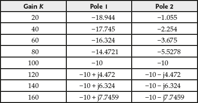
From Table 7.2, it is clear that one of the poles moves from left to right and the other one moves from right to left as closed-loop gain increases. But when ![]() = 100, both the values of poles are equal. If
= 100, both the values of poles are equal. If ![]() is increased further, poles moves into the complex plane where one pole moves in the direction of positive imaginary axis and the other one moves in the direction of negative imaginary axis.
is increased further, poles moves into the complex plane where one pole moves in the direction of positive imaginary axis and the other one moves in the direction of negative imaginary axis.
The root loci for the above closed-loop control system with the closed-loop poles are shown in Fig. 7.2. The gain ![]() = 100, is the breakaway point.
= 100, is the breakaway point.
The changes happening in the transient response of the system as the gain value varies can be inferred from the root locus. From Table 7.2, the following information is inferred and tabulated in Table 7.3.
Table 7.3 ∣ Nature of the system based on gain K


Fig. 7.2 ∣ Root loci of the closed-loop system
7.4 Basic Properties of Root Loci
The closed-loop transfer function of a simple control system is
 (7.1)
(7.1)
and its characteristic equation is given by
![]() (7.2)
(7.2)
The formulation of the root loci is based on the algebraic equation expressed as
![]() (7.3)
(7.3)
If ![]() contains a variable parameter
contains a variable parameter ![]() , then the function
, then the function ![]() can be rewritten as
can be rewritten as
 (7.4)
(7.4)
Substituting Eqn. (7.4) in Eqn. (7.2), we obtain

Hence, the characteristic equation of the system becomes

Here, the numerator is similar to the general algebraic equation used for formulating the root loci. Thus, the root loci for a control system can be identified by writing the loop transfer function ![]() in the form of
in the form of ![]() .
.
7.4.1 Conditions Required for Constructing the Root Loci
The characteristic equation of the closed-loop control system is expressed as the general algebraic equation used for constructing the root locus.
Here ![]() where
where![]() does not contain any variable parameter
does not contain any variable parameter ![]() and s is a complex variable.
and s is a complex variable.
Hence, the characteristic equation of the system becomes
![]()
Therefore, ![]()
From the above equation, two Evans conditions for constructing the root loci for the given system are obtained as follows:
Condition on Magnitude:
![]()
Conditions on Angles:

= Odd multiple of
 radians or 180°
= Even multiple of
 radians or 180°
where
 .
.
7.4.2 Usage of the Conditions
The following points help in the construction of root locus diagram in s - plane based on the above conditions.
- The trajectories of the root loci are determined by using the conditions on angles.
- The variable parameter
 on the root loci is determined by using the condition on magnitude. The value of
  is determined once the root loci are drawn.
7.4.3 Analytical Expression of the Conditions
Based on the knowledge of the poles and zeros of the loop transfer function, ![]() , the root locus for the system is graphically constructed. Hence, the conditions required for constructing the root loci are to be determined in the form of poles and zeros.
, the root locus for the system is graphically constructed. Hence, the conditions required for constructing the root loci are to be determined in the form of poles and zeros.
Let us express the transfer functions ![]() as
as

where ![]() and
and ![]()
The poles and zeros of ![]() can be real or purely imaginary or complex conjugate pairs.
can be real or purely imaginary or complex conjugate pairs.
Using the previous conditions for constructing the root loci, the conditions in terms of poles and zeros of ![]() are determined.
are determined.

The conditions on angles for different root loci are
- For
 (RL):
(RL):

- For
 (CRL)
(CRL)

where

Consider a point ![]() on the root loci drawn for a system whose characteristic equation is
on the root loci drawn for a system whose characteristic equation is ![]() .
.
For a positive ![]() , any point on the RL should satisfy the following condition:
, any point on the RL should satisfy the following condition:
The difference in radians or degrees between the sum of angles drawn from the zeros and sum of angles drawn from poles of ![]() to any point s1 in the RL should be an odd multiple of
to any point s1 in the RL should be an odd multiple of ![]() .
.
For a negative ![]() , any point on the CRL should satisfy the following condition:
, any point on the CRL should satisfy the following condition:
The difference in radians or degrees between the sum of angles drawn from the zeros and sum of angles drawn from poles of ![]() to any point s1 in the CRL should be an even multiple of
to any point s1 in the CRL should be an even multiple of ![]() .
.
7.4.4 Determination of Variable Parameter K
The variable parameter ![]() in the characteristic equation
in the characteristic equation ![]() can be determined for each point
can be determined for each point ![]() in the root loci by
in the root loci by

The value of ![]() at any point s1 in the root loci is obtained by substituting the value s1 in the above equation. The numerator and denominator of the above equation is graphically interpreted as the product of the length of the vectors drawn from the poles and zeros of
at any point s1 in the root loci is obtained by substituting the value s1 in the above equation. The numerator and denominator of the above equation is graphically interpreted as the product of the length of the vectors drawn from the poles and zeros of ![]() respectively.
respectively.
If the point s1 lies on the RL, then the variable parameter ![]() has a positive value. In addition, if the point s1 lies on the CRL, then the variable parameter
has a positive value. In addition, if the point s1 lies on the CRL, then the variable parameter ![]() has a negative value.
has a negative value.
Example of Constructing a Root Loci
Consider the function  .
.
Here the number of zeros ![]() and number of poles
and number of poles ![]() are 2 and 3 respectively.
are 2 and 3 respectively.
Consider an arbitrary point s1 in the ![]() -plane to verify the conditions. The vector lines are drawn from that point to each pole and zero present in the function as shown in Fig. 7.3.
-plane to verify the conditions. The vector lines are drawn from that point to each pole and zero present in the function as shown in Fig. 7.3.

Fig. 7.3 ∣ Vector lines from an arbitrary point
The angles from each pole or zero to that arbitrary point s1 are determined with respect to positive real axis and are denoted as ![]() for poles and
for poles and ![]() for zeros as represented in Fig. 7.3.
for zeros as represented in Fig. 7.3.
If the arbitrary point s1 is located in the RL, the angle condition for constructing the root loci is given by
![]()
![]()
where ![]() .
.
Similarly, if the arbitrary point ![]() is located in the CRL, the angle condition for constructing the root loci is given by
is located in the CRL, the angle condition for constructing the root loci is given by
![]()
![]()
where ![]()
Using the arbitrary point s1, the magnitude of the variable parameter K is obtained by

From Fig. 7.3, the lengths of vectors drawn from each pole and zero are noted down. Now, the variable parameter ![]() is given by
is given by

The sign of the variable parameter K depends on whether the root loci are RL or CRL.
In general, for the function ![]() with multiplying factor as the variable parameter K with the known poles and zeros of the function, the construction of root loci follows the two steps as given below:
with multiplying factor as the variable parameter K with the known poles and zeros of the function, the construction of root loci follows the two steps as given below:
- The arbitrary point
 in the
  -plane is identified, which satisfies the respective angle condition for different root loci (RL or CRL).
 - The variable parameter
 on the root loci is obtained using the formula.
Example 7.1: The loop transfer function of the system with a negative feedback system is given by  . Consider an arbitrary point
 ![]() in s-plane. Determine whether the point s1 lies in the RL or CRL.
in s-plane. Determine whether the point s1 lies in the RL or CRL.
Solution: The phase angle of the loop transfer function at ![]() is
is
![]()
= ![]()
= ![]()
= ![]()
Since this angle is neither an odd multiple nor an even multiple of ![]() , the arbitrary point
, the arbitrary point ![]() does not lie either on RL or CRL.
does not lie either on RL or CRL.
7.4.5 Minimum and Non-Minimum Phase Systems
If all the closed-loop zeros of the system lie in the left half of the ![]() -plane, then the system is called non-minimum phase system; and if any one of the closed-loop zeros of the system lies in the right half of the
-plane, then the system is called non-minimum phase system; and if any one of the closed-loop zeros of the system lies in the right half of the ![]() -plane, then the system is called minimum phase system.
-plane, then the system is called minimum phase system.
7.5 Manual Construction of Root Loci
The trial-and-error method of determining the variable parameter K and an arbitrary point ![]() in the s-plane that satisfies the angle condition for different types of root loci (RL or CRL) is a tedious process. To overcome these difficulties, Evans invented a special tool called Spirule (which assists in addition and subtraction of angles of vectors). But this method also has its difficulties to determine the unknown parameter K.
in the s-plane that satisfies the angle condition for different types of root loci (RL or CRL) is a tedious process. To overcome these difficulties, Evans invented a special tool called Spirule (which assists in addition and subtraction of angles of vectors). But this method also has its difficulties to determine the unknown parameter K.
7.5.1 Properties / Guidelines for Constructing the Root Loci
It is necessary to understand the properties, guidelines or rules for constructing the root loci for a system manually. The properties are based on the relation between the poles and zeros of ![]() and the roots of the characteristic equation
and the roots of the characteristic equation ![]() .
.
Property 1: The points on the root loci at ![]() and K = ± ∞
and K = ± ∞
- The points on the root loci corresponding to the variable parameter
 are the poles of
  .
. - The points on the root loci corresponding to the variable parameter
 are the zeros of
  .
.
Consider a system whose characteristic equation is given by
![]()
When K = 0, the roots of the given equation are ![]() ,
,![]() and
and ![]() . Similarly, when
. Similarly, when ![]() , the roots of the equation are
, the roots of the equation are ![]() . Since the order of the equation is 3, the third root lies at
. Since the order of the equation is 3, the third root lies at ![]() .
.
The above equation can be written as

Therefore, 
Thus, the poles and zeros of the given system are ![]() respectively.
respectively.
Hence, it is clear that the roots of the characteristic equation at ![]() are the poles of the transfer function
are the poles of the transfer function ![]() and the roots of the characteristic equation at
and the roots of the characteristic equation at ![]() including one at
including one at ![]() are the zeros of the of the transfer function
are the zeros of the of the transfer function![]() .
.
Property 2: Branches on the root loci
The locus of any one of the roots of the characteristic equation when the variable parameter K varies from ![]() is called the branch of the root loci.
is called the branch of the root loci.
The number of branches present in the root loci is equal to the number of poles or zeros present in the loop-transfer function depending on the values. Therefore, the condition by which the number of branches can be determined is given below:
Let ![]() be the number of poles present in the loop transfer function and
be the number of poles present in the loop transfer function and
![]() be the number of zeros present in the loop transfer function.
be the number of zeros present in the loop transfer function.
The number of branches of root loci is determined as:
If ![]() , number of branches of root loci = n
, number of branches of root loci = n
If ![]() , number of branches of root loci = m
, number of branches of root loci = m
If m = n, number of branches of root loci = m or n.
For the same characteristic equation of the system discussed in the previous property, ![]() , the number of branches of the root loci is equal to 3, since the order of the characteristic equation is 3.
, the number of branches of the root loci is equal to 3, since the order of the characteristic equation is 3.
Property 3: Root locus symmetry
The root locus of any system is symmetrical on the real axis of the s-plane. The root locus of the system may be symmetrical about the poles and zeros of the system or to any point on the real axis of the s-plane.
The root locus of any system may be symmetrical to one or more points on the real axis of the plane. It is also possible that the root locus may be symmetrical to a complex conjugate point.
Property 4: Intersection of asymptotes with the real axis of s-plane
All the asymptotes present in the root loci of any system will intersect at a particular point on the real axis of the s-plane. The particular point on the real axis where the asymptotes intersect is called centroid.
The formula for determining the centroid is given by
![]()
The centroid obtained using the above formula is a real number even when the poles or zeros are either real or complex conjugate pairs.
Property 5: Asymptotes of root loci and its angles and behaviour of root loci at ![]()
We know that the characteristic equation of any system ![]() can be replaced by
can be replaced by  , i.e.,
  . If the order of the polynomials
 ![]() are not equal (i.e.,
are not equal (i.e., ![]() ), then some of the branches of the root loci approach infinity in the s-plane.
), then some of the branches of the root loci approach infinity in the s-plane.
Asymptotes are used to describe the properties of root loci that approach infinity in the s-plane when ![]() . The number of asymptotes
. The number of asymptotes ![]() for a system when
for a system when ![]() will be
will be ![]() , which describes the root loci behaviour at
, which describes the root loci behaviour at ![]() . The angle of asymptotes is determined by
. The angle of asymptotes is determined by
![]() (7.5)
(7.5)
where ![]() , n is the number of finite poles of G(s)H(s) and m is the number of finite poles of G(s)H(s)
, n is the number of finite poles of G(s)H(s) and m is the number of finite poles of G(s)H(s)
The asymptotes are drawn from the centroid ![]() by using the angle of asymptotes.
by using the angle of asymptotes.
The asymptotes, the angle of asymptotes and the centroid (i.e., intersection of asymptotes on the real axis) for a transfer function  are shown in Fig. 7.4.
For the given example, the number of asymptotes ![]() , is 3(
, is 3(![]() ).
).
In Fig. 7.4, A1, A2 and A3 are the asymptotes whose angles are 60°, 180° and 300° which are obtained using Eqn. (7.5).
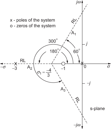
Fig. 7.4 ∣ Asymptotes, angle of asymptotes and centroid
Figs 7.5(a) through (c) show the asymptotes, the angle of asymptotes and the centroid for different types of system.

Property 6: Root loci on the real axis
In the root loci, each branch on the real axis starts from a pole and ends at a zero or infinity. Each branch on the real axis is determined based on a condition given below by assuming that we are searching for a branch of root loci on the real axis from right to left.
For a branch to exist on the real axis after a particular point, the summation of number of poles and zeros of ![]() to the right of that particular point should be an odd number.
to the right of that particular point should be an odd number.
The point at which the above condition is checked may be pole or zero which lies on the real axis. This condition for determining the branches of root loci on the real axis does not get affected by the complex poles and zeros of ![]() .
.
For the system whose transfer function is given by  , the branches of root loci are indicated in Fig. 7.6.

Fig. 7.6 ∣ Indication of branches of root loci on the real axis
Here, if we look to the right of the point −1 (zero of the system), only one pole exists (i.e., odd number). Hence, a branch of root loci exists between −1 and 0. Now, if we look from infinity, the total number of poles and zeros existing to the right of the point is 5 (odd number). Hence, a branch of root loci exists between ![]() .
.
Figures 7.7(a) and (b) indicate the branch of root loci existing on the real axis for two general systems.

From Figs. 7.7(a) and (b), it can be inferred that the addition of one pole at the origin changes the branch of root loci existing on the real axis.
Property 7: Angle of departure and angle of arrival in root loci
In a root locus, the angle of departure or arrival is determined for a complex pole or complex zero respectively. This angle indicates the angle of the tangent to the root locus.
The angle of departure ![]() and angle of arrival
and angle of arrival ![]() is determined using
is determined using
![]()
![]()
For the system whose poles are denoted as shown in Fig. 7.8(a), the angle of departure of the complex pole is determined using the formula.
The angle of departure for the pole ![]() is
is ![]() and the angle of departure for the pole
and the angle of departure for the pole ![]() is
is ![]() .
.
For the system whose zeros are denoted as shown in Fig. 7.8(b), the angle of arrival of the complex zero is determined using the formula.

Fig. 7.8(a) ∣ Angle of departure

Fig. 7.8(b) ∣ Angle of arrival
The angle of arrival for the zero ![]() is
is ![]() and the angle of arrival for the zero
and the angle of arrival for the zero ![]() is
is ![]() .
.
Property 8: Intersection of root loci with the imaginary axis
The intersection point of the root loci on the imaginary axis and the corresponding variable parameter K can be determined using two ways.
- Using Routh−Hurwitz criterion.
- Substituting
 in the characteristic equation and equating the real and complex parts to zero, the intersection point on the imaginary axis
  can be obtained and its corresponding gain value K.
Property 9: Breakaway or break-in points on the root loci
The point on the s-plane where two or more branches of the root loci arrive and then depart in the opposite direction is called breakaway point or saddle point. The point on the s-plane where two or more branches of the root loci arrive and then depart in opposite direction is called break-in point. The illustrations of different types of breakaway points are given in Table 7.4.
Table 7.4 ∣ Types of breakaway points
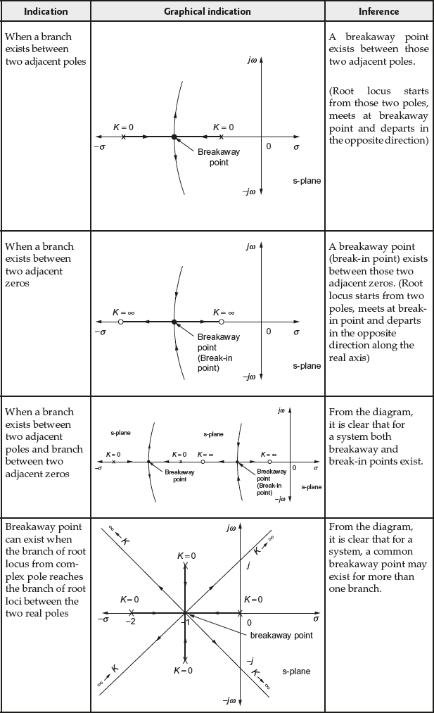
The root locus diagram for a particular system can have more than one breakaway point/break-in point and it is not necessary to have the breakaway point/break-in point only on the real axis. Due to the complex symmetry of root loci, the breakaway point/break-in point may be a complex conjugate pair.
The breakaway/break-in points on the root loci for a particular system whose characteristic equation is represented by ![]() must satisfy the following condition:
must satisfy the following condition:
![]() (7.6)
(7.6)
It is noted that all the breakaway/break-in points on the branch of the root loci must satisfy the above condition, but not all the solutions obtained using the equation are breakaway points. In other words, we can say that the above condition is necessary but not sufficient. Hence, in addition to the above condition, the breakaway point must also satisfy the condition, ![]() , for some real variable parameter K.
, for some real variable parameter K.
We know that ![]()
Taking the derivative on both sides of the equation with respect to the variable s, we obtain

Thus, the condition for breakaway point can also be written as
![]() (7.7)
(7.7)
All the solutions obtained by solving Eqn. (7.6) or Eqn. (7.7) cannot be valid breakaway/break-in points. Let ![]() be the solutions obtained by solving the equation. Each solution
be the solutions obtained by solving the equation. Each solution ![]() is said to be a valid or invalid breakaway point/break-in points based on the condition given in Table 7.5.
is said to be a valid or invalid breakaway point/break-in points based on the condition given in Table 7.5.
Table 7.5 ∣ Validation of breakaway point

Inference about the breakaway point
- If the solutions obtained using Eqn. (7.6) or Eqn. (7.7) are all real values and the value of
 at those real values are positive, then those values are called breakaway points on the root loci.
 - If the solutions obtained using Eqn. (7.6) or Eqn. (7.7) are complex conjugate values and if they also satisfy the condition
 (i.e., angle of
  at the breakaway point should be an odd multiple of 180°), then it is said to be a breakaway point of the root loci.
Gain at the breakaway point

Property 10: Root sensitivity
The root sensitivity is defined as the sensitivity of the roots of the characteristic equation when the variable parameter K varies. The root sensitivity is given by
![]()
Hence, at the breakaway point, the root sensitivity of the characteristic equation becomes infinite (since ![]() at breakaway point). The value of K should not be selected to operate the system at breakaway point.
at breakaway point). The value of K should not be selected to operate the system at breakaway point.
Property 11: Determination of variable parameter K on the root loci
If the root locus for the system is constructed manually, then the variable parameter K at any point ![]() on the root loci can be determined by
on the root loci can be determined by

But graphically, the variable parameter ![]() is determined by
is determined by

The properties to plot the root loci are tabulated in Table 7.6.
Table 7.6 ∣ Properties to construct root loci

7.5.2 Flow Chart for Constructing the Root Locus for a System
The flow chart for constructing the root locus for a system whose loop transfer function is known is shown in Fig. 7.9.


Fig. 7.9 ∣ Flow chart for construction of root locus
7.6 Root Loci for different Pole-Zero Configurations
The root loci for different pole-zero configuration are given in Table 7.7. The shape of the root loci for the system depends on the relative position of poles and zeros of the system.
Table 7.7 ∣ Root loci for different pole-zero configuration of the system

Example 7.2: Sketch the root locus of the system whose loop transfer function is given by  .
.
Solution:
- For the given system, poles are at
 , i.e., n = 4 and zeros do not exist, i.e.,
  .
. - Since
 , the number of branches of the root loci for the given system is
- For the given system, the details of the asymptotes are given below:
- Number of asymptotes for the given system

- Angles of asymptotes,

Therefore,

- Centroid,


- Number of asymptotes for the given system
- Since complex poles exist, angle of departure exists for the system.
To determine the angle of departure
 :
:- For the pole
 ,
,


- For the pole
 ,
, 
- For the pole
- To determine the number of branches existing on the real axis:
If we look from the pole p = 0, the total number of poles and zeros existing on the right of 0 is zero (nor an even number or an odd number). Therefore, a branch of root loci does not exist between 0 and
 .
.Similarly, if we look from the pole p = −4, the total number of poles and zeros existing on the right of −4 is three (odd number). Therefore, a branch of root loci exists between 0 and −4.
Hence, only one branch of root loci exists on the real axis for the given system.
- The breakaway and break-in points for the given system are determined by
 (1)
(1)For the given system, the characteristic equation is
 (2)
(2)i.e.,

Therefore,
 (3)
(3)Differentiating the above equation with respect to
 and using Eqn. (1), we obtain

Upon solving, we obtain

Substituting s = −2 in Eqn. (3), we get K = 64. Since
 is positive, the point
  is a breakaway point.
Since two of the three obtained solution are complex numbers, it is necessary to check the angle condition also. Therefore,

Also,


Since the angle for the given system at the complex numbers are odd multiple of 180°, the obtained complex numbers are also breakaway points.
Hence,
 and
and  are the breaking away points for the given system.
 - The point at which the branch of root locus intersects the imaginary axis is determined as follows:
From Eqn. (2), the characteristic equation of the system is
 (4)
(4)Routh array for the above equation,

To determine the point at which root locus crosses the imaginary axis, the first element in all the rows of Routh array must be either zero or greater than zero. i.e.,
![]() . Therefore,
. Therefore, ![]()
Substituting K in the characteristic equation, we obtain
![]()
Substituting ![]() in the above equation, we get
in the above equation, we get
![]()
![]()
Equating the imaginary part of the above equation to zero, we get
![]()
![]()
or ![]()
Therefore, the point at which the root locus crosses the imaginary axis is ![]() .
.
The entire root locus for the system is shown in Fig. E7.2.
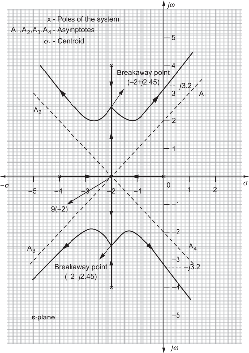
Fig. E7.2
Example 7.3: A pole-zero plot of a loop transfer function with gain K in the forward path of a control system is shown in Fig. E7.3(a). Sketch the root locus for the system.

Fig. E7.3(a)
Solution:
- In the pole-zero plot shown in Fig. E7.3(a), the poles are at
 i.e.,
i.e., and zeros are at
  ,
,  i.e.,
i.e.,  . Therefore, the loop transfer function,
  .
. - Since
 the number of branches of the root loci for the given system is
  .
. - For the given system, as the number of poles and number of zeros are equal, the number of asymptotes for the given system is zero. Hence, it is not necessary of calculating the angle of asymptotes and centroid for the given system.
- As all the poles and zeros are real values, there is no necessity in calculating the angle of departure and angle of arrival.
- Though the number of branches of the root loci for the given system is 2, it is necessary to determine the number of branches of the root loci existing on the real axis.
If we look from the point p = −1, the total number of poles and zeros existing on the right of −1 is zero (neither odd nor even). Therefore, a branch of root locus does not exists between −1 and
 .
.Similarly, if we look from the point p = −3, the total number of poles and zeros existing on the right of −3 is one (odd number). Therefore, a branch of root loci exists between −3 and −1.
Similarly, if we look from the point z = −4, the total number of poles and zeros existing on the right of −4 is two (even number). Therefore, a branch of root loci does not exist between −4 and −3.
Similarly, if we look from the point z = −5, the total number of poles and zeros existing on the right of −5 is three (odd number). Therefore, a branch of root loci exists between −5 and −4.
Similarly, if we look from the point at −∞, the total number of poles and zeros existing on the right of the point is four (even number). Therefore, a branch of root loci does not exist between −∞ and −5.
Hence, two branches of root loci exist on the real axis for the given system.
- The breakaway/break-in points for the given system are determined by,
 (1)
(1)For the given system, the characteristic equation is
 (2)
(2)i.e.,

Therefore,
 (3)
(3)Differentiating the above equation with respect to
 and using Eqn. (1), we get

i.e.,

Upon solving, we get

Substituting the values of s in Eqn. (3), we get the corresponding values of K as
K = 0.202 for s = −2.42 and K = 143.07 for s = −4.38
The breakaway point exists only for the positive values of K. Hence, s = −2.42 and s = −4.38 are the two breakaway points that exist for the given system.
- The point at which the branch of root loci intersects the imaginary axis is determined as follows:
From Eqn. (2), the characteristic equation for the given system is

i.e.,

Routh array for the above equation is

For


For


For
 ,
, 

As there exists no positive marginal value of K, the root locus does not get intersected with the imaginary axis. Also, the complete root locus lies in the left half of s-plane.
The final root locus for the system is shown in Fig. E7.3(b).

Fig. E7.3(b)
Example 7.4: A unity feedback control system shown in Fig. E7.4(a) has a controller with a transfer function ![]() , which controls a process with the transfer function
, which controls a process with the transfer function  . Find the loop transfer function of the system and construct the root locus of the system.

Fig. E7.4(a)
Solution: For the given system ![]() and
and  . Therefore, the loop transfer function
  .
.
- For the loop transfer function of the system, the poles are at 0,
 i.e.,
i.e.,  and zero does not exist i.e.,
  .
. - Since
 the number of branches of the root loci for the given system is
  .
. - For the given system, the details of the asymptotes are given below:
- Number of asymptotes for the given system is
 .
. - Angles of asymptotes
 for
for 
Therefore,

- Centroid

- Number of asymptotes for the given system is
- Since complex poles exist, the angle of departure exists for the system.
To determine the angle of departure
 :
:- For the pole
 ,
,


- For the pole
 ,
, 
- For the pole
- To determine the number of branches existing on the real axis:
If we look from the point p = 0, the total number of poles and zeros existing on the right of 0 is zero (neither odd nor an even number). Therefore, a branch of root loci does not exist between 0 and
 .
.Similarly, if we look from the point at −
 , the total number of poles and zeros existing on the right of the point is three. Therefore, a branch of root loci exists between −
 and 0.
Hence, only one branch of root loci exists on the real axis for the given system.
- The breakaway or break-in points are determined by
 (1)
(1)For the given system, the characteristic equation is
 (2)
(2)i.e.,

Therefore,

Differentiating the above equation with respect to
 and using Eqn. (1), we obtain

Upon solving, we obtain

Since the above points are complex conjugate values, the angle condition should be checked.
i.e.,


Also,

Since the angle of
 is not an odd multiple of
  , the points obtained using Eqn. (1) is not a breakaway point.
Hence, no breakaway point exists for the given system.
- The point at which the branch of root loci intersects the imaginary axis is determined as follows:
From Eqn. (2), the characteristic equation for the given system is

Routh array for the above equation is

Depending on K, the system can be stable or marginally stable or unstable.
From Routh array, if the value of
- K is between 0 and 3, the system is stable.
- K is greater than 4, the system is unstable.
Now, if K = 4, the third row of Routh array becomes 0. Hence, the auxiliary equation is
 i.e.,
i.e.,  .
.Solving the above equation, we obtain
 , which is the intersection point on the imaginary axis.
The final root locus for the system is shown in Fig. E7.4(b).

Fig. E7.4(b)
Example 7.5: Develop the root locus for the system whose loop transfer function is given by 
Solution:
- For the given system, the poles are at 0, −1 and −4 i.e.,
 and zero is at −2 i.e.,
  .
. - Since
 , the number of branches of the root loci for the given system is
- The details of the asymptotes are given below:
- Number of asymptotes for the given system
 .
. - Angles of asymptotes
 for
for 
Therefore,

- Centroid

- Number of asymptotes for the given system
- As all the poles and zeros are real values, there is no necessity to calculate the angle of departure and angle of arrival.
- To determine the number of branches existing on the real axis:
If we look from the pole p = −1, the total number of poles and zeros existing on the right of −1 is one (odd number). Therefore, a branch of root loci exists between −1 and 0.
Similarly, if we look from the pole p = −4, the total number of poles and zeros existing on the right of −4 is three (odd number). Therefore, a branch of root loci exists between −4 and −2.
Hence, two branches of root loci exist on the real axis for the given system.
- The breakaway point for the given system is determined by
 (1)
(1)For the given system, the characteristic equation is
 (2)
(2)i.e.,

Therefore,

Differentiating the above equation with respect to
 and using Eqn. (1), we obtain

The above equation can be solved using Lin's method (trial-and-error method). The third-order polynomial of the above equation will have at least one real root. The trial and error method for determining the roots is shown below:
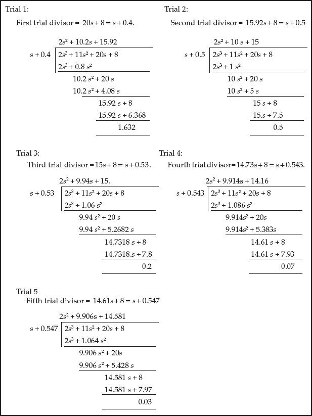
Since the remainder obtained in the fifth trial is
 , the point
  is one of the roots of the equation.
Hence, rewriting the above cubic equation, we obtain

Solving the above equation, we obtain

Substituting s = −0.549 in Eqn. (3), we get K = 0.5888. Since
 is positive, the point
  is a breakaway point.
As the other two points are complex conjugate points, it is necessary to determine the angles of the system at those points.
i.e.,

Also,

Since the angles obtained are not odd multiple of
 , the complex points obtained using Eqn. (1) are not a breakaway or break-in points.
Hence, only one breakaway point exists for the given system.
- The point at which the branch of root loci intersects the imaginary axis is obtained as follows:
Using Eqn. (2), the characteristic equation for the given system is

i.e.,

Routh array for the above equation is

To determine the point at which the root locus crosses the imaginary axis, the first element in the third row must be zero, i.e.,
 . Therefore,
  . As K is a negative real value, the root locus do not cross the imaginary axis.
The final root locus for the system is shown in Fig. E7.5.

Fig. E7.5
Example 7.6: Sketch the root locus for the system whose loop transfer function ![]() . Also, (i) determine gain
. Also, (i) determine gain ![]() when
when ![]() , (ii) determine the settling time
, (ii) determine the settling time ![]() and peak time
and peak time ![]() using the gain value obtained in (i).
using the gain value obtained in (i).
Solution:
- For the given system
 , the poles are at 0, −2 and −4 i.e.,
  and zeros do not exist i.e.,
  .
. - Since
 , the number of branches of the root loci for the given system is
  .
. - The details of the asymptotes are given below:
- Number of asymptotes for the given system
 .
. - Angles of asymptotes
 for
for
Therefore,

- Centroid

- Number of asymptotes for the given system
- As all the poles and zeros are real values, there is no necessity in calculating the angle of departure and angle of arrival.
- To determine the number of branches existing on the real axis:
If we look from the pole p = −2, the total number of poles and zeros existing on the right of −2 is one (odd number). Therefore, a branch of root loci exists between −2 and 0.
Similarly, if we look from the point at
 , the total number of poles and zero existing on the right of the point is three (odd number). Therefore, a branch of root loci exists between
  and −4.
Hence, two branches of root loci exist on the real axis for the given system.
- The breakaway/break-in points for the given system are determined by
 (1)
(1)For the given system, the characteristic equation is
 (2)
(2)i.e.,

Therefore,
 (3)
(3)Differentiating the above equation with respect to
 and using Eqn. (1), we obtain

Solving for s, we get

Substituting the values of s in Eqn. (3), we get the corresponding values of K as
K = 3.0792 for s = −0.8453 and K = −3.0792 for s = −3.1547.
The breakaway point exists only for the positive values of K. Hence, s = −0.8453 is the only one breakaway point that exists for the given system.
- The point at which the branch of root loci intersects the imaginary axis is determined as follows:
From Eqn. (2), the characteristic equation for the given system is

i.e.,
 (4)
(4)Routh array for the above equation is

To determine the point at which the root locus crosses the imaginary axis, the first element in the third row must be zero, i.e.,
 . Therefore,
Substituting K in Eqn. (3), we get
s3 + 6s2 + 8s + 48 = 0
Upon solving, we get
s = −6, j2.828 , −j2.828.
Hence, the root locus crosses the imaginary axis at
 .
.The complete root locus for the system is shown in Fig. E7.6(a).

Fig. E7.6(a)
- It is given that the maximum peak overshoot for the system is
 . We know that the maximum peak overshoot for a second-order system is

Substituting the known values, we obtain


Solving the above equation, we obtain

For this damping ratio
 a straight line can be drawn from the origin with the angle,
  , obtained by
  . The point at which the straight line crosses on the root locus is
  as shown in Fig. E7.6(b).
Fig. E7.6(b)
We know that the magnitude condition at any point of the system

i.e.,

Therefore,

Therefore, gain K corresponding to the given peak overshoot,
 is K = 9.174.
 - The point at which the line for
 cuts the root locus is
  . The settling time and peak time of the system is obtained as


- It is given that the maximum peak overshoot for the system is
Example 7.7: Prove that the breakaway points for a system in the root locus are obtained by solving for the solutions of ![]() where K is the open-loop gain (variable parameter) of the system whose open-loop transfer function is
where K is the open-loop gain (variable parameter) of the system whose open-loop transfer function is ![]() .
.
Solution: The characteristic equation of the system whose open-loop transfer function of the system given by ![]() is obtained as
is obtained as ![]() which is the combination of s terms and open-loop gain K terms. It can be arranged as
which is the combination of s terms and open-loop gain K terms. It can be arranged as
![]() (1)
(1)
where P(s) is the polynomial containing K and s terms and
KQ(s) is the polynomial containing K and s terms
Now at breakaway points, multiple roots occur. Mathematically, this is possible if ![]() .
.
Differentiating Eqn. (1) with respect to s, we get
![]()
Therefore,  (2)
(2)
Substituting Eqn. (2) in Eqn. (1) at breakaway point, we can write
 (3)
(3)
Solving Eqn. (3) for s, breakaway points can be obtained.
Now, equating Eqn. (1) to zero and solving for K, we get

Therefore,  (4)
(4)
i.e., ![]() (5)
(5)
This is same as Eqn. (3) which yields breakaway points. This proves that the roots of ![]() are the actual breakaway points.
are the actual breakaway points.
Example 7.8: (i) Prove that the root locus of the system  is a circle. (ii) Assuming a = 4 and b = 6 for the above loop transfer function, develop the root locus. (iii) Determine the range of variable gain, K for which the system is under-damped. (iv) Determine the range of variable gain, K for which the system is critically damped and (v) Determine the minimum value of damping ratio.
Solution:
- Let
 be a complex point on the root locus for the given system.
Therefore,

To prove that the root locus of the system is a circle, the angle of the system at any point must be 180°.
i.e.,
 (1)
(1)Therefore,


From Eqn. (1),

Therefore,

Since
 , we obtain
Therefore,

Adding and subtracting
 on both sides, we obtain
Therefore,

The above equation is the equation of a circle with centre
 which is the location of open loop zero and radius
  . This proves that root locus of the given system is a circle.
 - Assuming a = 4 and b = 6, the loop transfer function of the system becomes
 .
.
- For the given system, the poles are at 0 and −4, i.e.,
 and zero is at −6, i.e.,
  .
. - Since
 , the number of branches of the root loci for the given system
- For the given system, the details of the asymptotes are given below.
- Number of asymptotes for the given system
 .
. - Angles of asymptotes
 for
for 
Therefore,

- Centroid

- Number of asymptotes for the given system
- Since no complex pole or complex zero exists for the given system, there is no necessity of calculating the angle of departure or angle of arrival.
- To determine the number of branches existing on the real axis:
If we look from the pole p = −4, the total number of poles and zeros existing on the right of the point is one (odd number). Therefore, a branch of root loci exists between −4 and 0.
Similarly, if we look from the point at
 , the total number of poles and zeros existing on the right of the point is three (odd number). Therefore, a branch of root loci exists between −6 and
Hence, two branches of root loci exist on the real axis for the given system.
- The breakaway and break-in points for the given system are determined by
 (1)
(1)For the given system, the characteristic equation is
 (2)
(2)i.e.,

Therefore,
 (3)
(3)Differentiating the above equation with respect to
 and using Eqn. (1), we obtain

Upon solving, we obtain

Substituting the values of s in Eqn. (3), we get the corresponding values of K as
K = 1.071 for s = −2.5358 and K = 14.928 for s = −9.4641.
The breakaway point exists only for the positive values of K. Hence, s = −2.5358 and s = −9.4641 are the two breakaway points that exist for the given system.
- The point at which the branch of root loci intersects the imaginary axis is determined as follows:
From Eqn. (2), the characteristic equation for the given system is
 (4)
(4)Routh array for the above equation is

To determine the point at which the root locus crosses the imaginary axis, the first element in the second row must be zero, i.e.,
 .
.As K is a negative real value, the root loci does not cross the imaginary axis.
Hence, the final root loci for the system are shown in Fig. E7.8.

Fig. E7.8
- For the given system, the poles are at 0 and −4, i.e.,
- For the system to be under-damped, the range of gain K is

- The system is critically damped when the gain K = 1.0717 or 14.928.
- Determination of minimum value of damping ratio

For the root locus of the given system a tangent is drawn from the origin to the root locus and the angle from the real axis to the tangent is measured as
 as shown in Fig. E7.8.
Therefore, the damping ratio,
 .
.
Example 7.9: Plot the root locus for the system whose loop transfer function is ![]() . Also, determine the variable parameter K(i) for marginal stability of the system and (ii) at the point s = −4.
. Also, determine the variable parameter K(i) for marginal stability of the system and (ii) at the point s = −4.
Solution:
- For the given system, the poles are at 0, −1 and −3 i.e.,
 and zero does not exist i.e.,
  .
. - Since
 , the number of branches of the root loci for the given system is
  .
. - For the given system, the details of the asymptotes are given below:
- Number of asymptotes for the given system
 .
. - Angles of asymptotes
 for
for 
Therefore,

- Centroid

- Number of asymptotes for the given system
- Since no complex pole or complex zero exists for the given system, there is no necessity of calculating the angle of departure or angle of arrival.
- To determine the number of branches existing on the real axis:
If we look from the pole p = −1, the total number of poles and zeros existing on the right of −1 is one (odd number). Therefore, a branch of root loci exists between −1 and 0.
Similarly, if we look from the point at
 , the total number of poles and zeros existing on the right of the point is three. Therefore, a branch of root loci exists between
  and −3.
Hence, two branches of root loci exist on the real axis for the given system.
- The breakaway/break-in points for the given system are determined by
 (1)
(1)For the given system, the characteristic equation is
 (2)
(2)i.e.,

Therefore,
 (3)
(3)Differentiating the above equation with respect to
 and using Eqn. (1), we obtain

Upon solving, we obtain

Substituting the values of s in Eqn. (3), we get the corresponding values of K as
K = 0.63311 for s = −0.451 and K = −2.11 for s = −2.215
The breakaway point exists only for the positive values of K. Hence, s = −0.451 is the only one breakaway point that exists for the given system.
- The point at which the branch of root locus crosses the imaginary axis is determined as follows:
From Eqn. (2), the characteristic equation for the given system is

Therefore,
 (4)
(4)Routh array for the above equation is

To determine the point at which the root locus crosses the imaginary axis, the first element in the third row must be zero, i.e.,
 Therefore,
Substituting K in Eqn. (3), we get
s3 + 4s2 +3s +12 = 0
Upon solving, we get
s = −4, j1.732 , −j1.732.
Hence, the root locus crosses the imaginary axis at
 .
.The root locus plot for the system is shown in Fig. E7.9.

Fig. E7.9
- The marginal value of variable gain K = 12.
- The variable gain K at any point s is obtained by

Hence, at s = −4, we obtain

K = 12.
Example 7.10: Sketch the root locus of the system whose loop transfer function is given by ![]() . Also, determine ω at
. Also, determine ω at ![]() .
.
Solution:
- For the given system, poles are at
 and
and  i.e.,
i.e.,  and zero is at −2 i.e.,
  .
. - Since
 , the number of branches of the root loci for the given system is
  .
. - For the given system, the details of the asymptotes are given below:
- Number of asymptotes for the given system

- Angles of asymptotes
 for
for 
Therefore,
 .
. - Centroid

- Number of asymptotes for the given system
- Since complex poles exist, the angle of departure exists for the system.
To determine the angle of departure θd:
- For the pole


- For the pole

 .
.
- For the pole
- To determine the number of branches existing on the real axis:
If we look from point at
 , the total number of poles and zeros existing on the right of the point is three (odd number). Therefore, a branch of root loci exists between
  and −2.
Hence, one branch of root loci exists on the real axis for the given system.
- The breakaway/break-in points for the given system are determined by
 (1)
(1)For the given system, the characteristic equation is
 (2)
(2)i.e.,

Therefore,
 (3)
(3)Differentiating the above equation with respect to
 and using Eqn. (1), we obtain

Upon solving, we obtain
 and −3.73
Substituting the values of s in Eqn. (3), we get the corresponding values of K as
K = 10.62 for s = −3.73 and K = −1.464 for s = −0.26
The breakaway point exists only for the positive values of K. Hence, s = −3.73 is the only one breakaway point that exists for the given system.
- The point at which the branch of root locus crosses the imaginary axis is determined as follows:
From Eqn. (2), the characteristic equation of the system is
 (4)
(4)Routh array for the above equation is

To determine the point at which root locus crosses the imaginary axis, the first element in the second row and third row must be zero, i.e.,
 and
and  . Solving for
  , we obtain
  and
and  . Since
  lies within
  , we take .
As K is negative real value, the root loci do not cross the imaginary axis.
The final root locus for the system is shown in Fig. E7.10.

Fig. E7.10
To determinine damping ratio ω
The characteristic equation of a second-order system is
![]() (5)
(5)
where ![]() is the undamped natural frequency of the system and
is the undamped natural frequency of the system and ![]() is the damping ratio.
is the damping ratio.
The characteristic equation of the given system after substituting ![]() , is
, is
![]() (6)
(6)
Comparing Eqs. (5) and (6), we obtain
![]()
Given K = 1.33, Hence ![]() i.e., ωn= 2.379
i.e., ωn= 2.379
Then, ![]()
Therefore, the damping ratio, ![]()
Example 7.11: Plot the root locus of the system whose loop transfer function is given by ![]() .
.
Solution:
- For the given system, poles are at 0, −1, −3 and −5 i.e.,
 and zeros do not exist i.e.,
  .
.
Since
 , the number of branches of the root loci for the given system is
  .
. - For the given system, the details of the asymptotes are given below:
- Number of asymptotes for the given system
 .
. - Angles of asymptotes,
 for
for 
Therefore,

- Centroid

- Number of asymptotes for the given system
- Since no complex pole or complex zero exists for the system, there is no necessity of determining angle of departure/angle of arrival.
- To determine the number of branches existing on the real axis:
Since the total number of poles and zeros existing on the right of −1 and −5 are 1 and 3 (odd numbers), a branch of root loci exists between −1 and 0, and −5 and −3.
Hence, two branches of root loci exist for a given system on the real axis.
- The breakaway/break-in points for the given system are determined by
 (1)
(1)For the given system, the characteristic equation is
 (2)
(2)i.e.,

Therefore,
 (3)
(3)Differentiating the above equation with respect to
 and using Eqn. (1), we obtain
Upon solving, we obtain

Substituting the values of s in Eqn. (3), we get the corresponding values of K as
K = 2.878 for s = −0.425, K = 12.949 for s = −4.253 and K = −6.035 for s = −2.07
The breakaway points exist only for the positive values of K. Hence, s = −0.425 and s = −4.253 are the two breakaway points that exist for the given system.
- The point at which the branch of root locus crosses the imaginary axis is determined as follows:
To find the crossing point on the imaginary axis, substitute
 in
in


Equating imaginary part to zero, we obtain


or

Hence, the root locus intersects at
 .
.Equating real parts to zero, we obtain

K = 35.55.
Hence, the gain of the system at which the root locus intersects the imaginary axis is 35.55.
The complete root locus for the system is shown in Fig. E7.11.

Fig. E7.11
Example 7.12: Sketch the root locus of the system whose loop transfer function is given by ![]() .
.
Solution:
- For the given system, poles are at 0, −1 and −2, i.e.,
 and zeros do not exist i.e.,
  .
.
Since
 , the number of branches of the root loci for the given system is
  .
. - For the given system, the details of the asymptotes are given below:
- Number of asymptotes for the given system

- Angles of asymptotes
 for
for 
Therefore,

- Centroid

- Number of asymptotes for the given system
- Since no complex pole or complex zero exists for the system, there is no necessity in determining the angle of departure/angle of arrival.
- To determine the number of branches existing on the real axis:
If we look from the pole p = −1, the total number of poles and zeros existing on the right of −1 is one (odd number). Therefore, a branch of root loci exists between −1 and 0.
Similarly, if we look from the pole p = −
 , the total number of poles and zeros existing on the right of the point is three (odd number). Therefore, a branch of root loci exists between −
 and −2.
Hence, two branches of root loci exist on the real axis for the given system.
- The breakaway/break-in points for the given system can be determined by
 (1)
(1)For the given system, the characteristic equation is
 (2)
(2)i.e.,

Therefore,
 (3)
(3)Differentiating the above equation with respect to
 and using Eqn. (1), we obtain
Upon solving, we obtain

Substituting the values of s in Eqn. (3), we get the corresponding values of K as
K = 0.384 for s = −0.42 and K = −0.375 for s = −1.5
The breakaway point exists only for the positive values of K. Hence, s = −0.42 is the only one breakaway point that exists for the given system.
- The point at which the branch of root locus crosses the imaginary axis can be determined as follows:
From Eqn. (2), the characteristic equation of the system is
 (4)
(4)Routh array for the above equation is

To determine the point at which root locus crosses the imaginary axis, the first element in the third row must be zero, i.e.,
 . Therefore,
Substituting K in Eqn. (4) and solving for
 , we obtain
Hence, the root locus crosses the imaginary axis at
 .
.The final root locus for the system is shown in Fig. E7.12.

Fig. E7.12
Example 7.13: The characteristic polynomial of a feedback control system is given by ![]() . Plot the root locus for this system.
. Plot the root locus for this system.
Solution: The characteristic polynomial for the given system is
![]()
i.e., ![]()
![]()
![]()
i. e., 
We know that the characteristic equation is ![]() .
.
Therefore, 
- For
 , poles are at 0 and −1, i.e.,
  and zeros are at −2 and −3, i.e.,
  .
. - Since
 , the number of branches of the root loci for the given system is
- Since the number of poles and number of zeros present in the system are equal, no asymptote exists for the system and hence the angle of asymptotes and centroid need not be determined for the system.
- Since no complex pole or complex zero exists for the system, there is no necessity of determining angle of departure/angle of arrival.
- To determine the number of branches existing on the real axis:
Since the total number of poles and zeros existing on the right of −1 and −3 are 1 and 3 (odd numbers), a branch of root loci exists between −1 and 0 and −3 and −2.
Hence, two branches of root loci exist on the real axis for the given system.
- The breakaway and break-in points for the given system can be determined by
 (1)
(1)For the given system, the characteristic equation is
 (2)
(2)i.e.,

Therefore,
 (3)
(3)Differentiating the above equation with respect to
 and using Eqn. (1), we obtain


Upon solving, we get

For
 and
and  , the values of K are 0.0717 and 13.93 respectively. Since the values of
  are positive, the points
  and
and  are breakaway point and break-in point.
 - The point at which the branch of root loci crosses the imaginary axis is determined as follows:
From Eqn. (2), the characteristic equation of the system is
 (4)
(4)Routh array for the above equation,

To determine the point at which root locus crosses the imaginary axis, the first element in all the rows must be zero, i.e.,
 . Therefore,
  .
.Since K is negative, the root locus does not cross the imaginary axis.
The complete root locus for the system is shown in Fig. E7.13.

Fig. E7.13
Example 7.14: Sketch the root locus of the system whose transfer function is given by  .
.
Solution: We know that, the closed-loop transfer function of the system with the feedback transfer function ![]() and open loop transfer function
and open loop transfer function ![]() is given by
is given by

Converting the given transfer function to the above form, we obtain

Hence, the function  for which the root locus has been drawn in the subsequent steps:
- For the given system
 , poles are at
  i.e.,
i.e.,  and zeros do not exist i.e.,
  .
. - Since
 , the number of branches of the root loci for the given system is
  .
. - For the given system, the details of the asymptotes are given below:
- Number of asymptotes for the given system

- Angles of asymptotes
 for
for 
Therefore,

- Centroid


- Number of asymptotes for the given system
- Since complex poles exist, the angle of departure exists for the system.
To determine the angle of departure
 :
:- For the pole


- For the pole
 ,
, 
- For the pole
- To determine the number of branches existing on the real axis:
Since the total number of poles and zeros existing on the right of −4 is 3 (odd number), a branch of root loci exists between −4 and 0.
Hence, one branch of root loci exists on the real axis for the given system.
- The breakaway point/break-in points for the given system can be determined by
 (1)
(1)For the given system, the characteristic equation is
 (2)
(2)i.e.,

Therefore,
 (3)
(3)Differentiating the above equation with respect to
 and using Eqn. (1), we obtain
Upon solving, we obtain

For
 ,
,  is 21.01. Since
  is positive, the point at
  is a breakaway point.
Since the other two points obtained by solving Eqn. (1) are complex numbers, it is necessary to check the angle condition also.
Hence,


Similarly,

Since the angles obtained for the given system at the complex numbers obtained on solving Eqn. (1) are not odd multiple of 180°, the complex numbers are not breakaway points.
Hence, only one breakaway point exists for the given system.
- The point at which the branch of root loci intersects the imaginary axis can be determined as follows:
From Eqn. (2), the characteristic equation of the system is
 (4)
(4)Routh array for the above equation is

To determine the point at which root locus crosses the imaginary axis, the first element in all the rows must be zero, i.e.,
 . Therefore,
  .
.Substituting K in the characteristic equation, we obtain

Substituting s = jω in the above equation, we obtain


Equating the imaginary part of the above equation to zero, we obtain


or

Therefore, the point at which the root locus crosses the imaginary axis is
 .
.The complete root locus for the system is shown in Fig. E7.14.
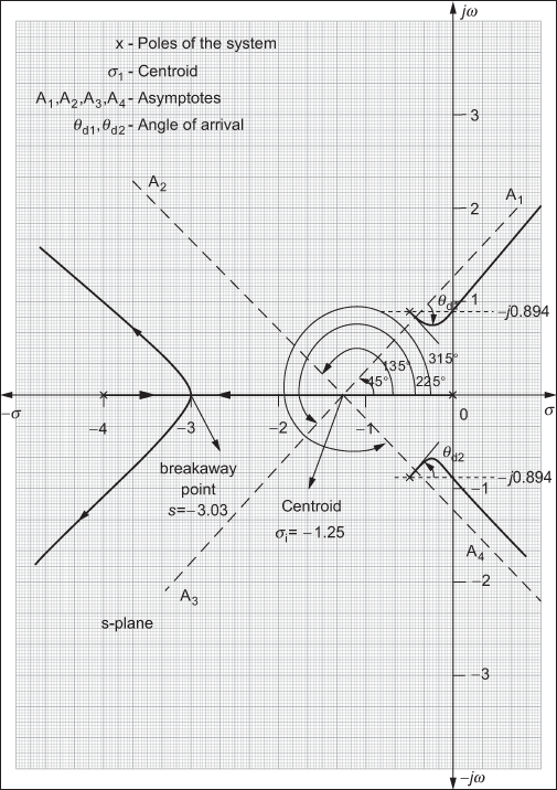
Fig. E7.14
Example 7.15: Sketch the root locus of the system whose loop transfer function is given by  . Also, determine gain K
(i) when the damping ratio is ξ = 0.707 and (ii) for which repetitive roots occur.
Solution The given function can be rewritten as

Replacing ![]() by K' in the above equation, we obtain
by K' in the above equation, we obtain

- For the given system, poles are at 0 and −2 i.e.,
 and zeros are at
  i.e.,
i.e.,  .
. - Since
 , the number of branches of the root loci for the given system is
  .
. - Since the number of poles and zeros present in the system are equal, the given system does not have any asymptote. Also, for the given system, it is not possible to determine the angle of asymptotes and centroid
- Since complex zeros exist, the angle of arrival exists for the system.
To determine the angle of arrival
 :
:- For the zero
 ,
,


- For the zero
 ,
, 
- For the zero
- To determine the number of branches existing on the real axis:
Since the total number of poles and zeros existing on the right of −2 is 3 (odd number), a branch of root loci exists between −2 and 0.
Hence, one branch of root loci exists on the real axis for the given system.
- The breakaway/break-in points for the given system can be determined by
 (1)
(1)For the given system, the characteristic equation is
 (2)
(2)i.e.,

Therefore,
 (3)
(3)Differentiating the above equation with respect to
 and using Eqn. (1), we get


Upon solving, we obtain

Substituting the values of s in Eqn. (3), we get the corresponding values of K as
K = −1.6 for s = 2 and K = 0.5 for s = −1
The breakaway point exists only for the positive values of K. Hence, s = −1 is the only one breakaway point that exists for the given system.
- The point at which the root loci intersects the imaginary axis can be obtained as follows:
From Eqn. (2), the characteristic equation of the system is

Routh array for the above equation is

To determine the point at which root locus crosses the imaginary axis, the first element in all the rows must be zero, i.e.,
 . Therefore,
Thus,

Since K is negative, the root locus does not cross the imaginary axis at any point.
The complete root locus for the system is shown in Fig. E7.15.

Fig. E7.15
- Determinine K:
Given the damping ratio
 angle
angle 
 .
.Draw a line from origin at an angle of 45° so that the line bisects the root locus.
Determine the point at which the root locus has been bisected. For the given problem, the root locus gets bisected at
 .
.Hence, the magnitude of the given transfer function at that particular point is 1.
 at
at


Therefore, the value of K for the given damping ratio is

- Finding gain at which the repetitive roots occur:
For a given system, the repetitive roots occur only at breakaway or break-in points.
Therefore,

i.e.,


Therefore, the value of
 at which repetitive roots occur is
 .
.
Example 7.16: Construct the root locus of the system whose loop transfer function is given by  .
.
Solution:
- For the given system, poles are at 0, 0 and −10 i.e.,
 and zero is at −2 i.e.,
  .
. - Since
 , the number of branches of the root loci for the given system is
- For the given system, the details of the asymptotes are given below:
- Number of asymptotes for the given system

- Angles of asymptotes
 for
for 
Therefore,
 and
and 
- Centroid


- Number of asymptotes for the given system
- Since a complex pole or complex zero does not exist for the given system, there is no angle of departure/angle of arrival.
- To determine the number of branches existing on the real axis:
If we look from the pole p = −10, the total number of poles and zeros existing on the right of −10 is three (odd number). Therefore, a branch of root loci exists between −10 and −2.
Hence, only one branch of root loci exists on the real axis for the given system.
- The breakaway/break-in points for the given system can be determined by
 (1)
(1)For the given system, the characteristic equation is
 (2)
(2)i.e.,

Therefore
 (3)
(3)Differentiating the above equation with respect to
 and using Eqn. (1), we obtain


Upon solving, we obtain

Substituting
 in Eqn. (3), we obtain
  . Hence, the point is not a valid breakaway point.
For the other two points, i.e.,
 , it is necessary to check the angle condition.
Similarly,

Since the angle of the system at the complex numbers is not an odd multiple of 180°, these complex numbers are not valid breakaway points.
Hence, no breakaway point exists for the given system.
- The point at which the branch of root loci intersects the imaginary axis can be determined as follows:
From Eqn. (2), the characteristic equation of the system is
 (4)
(4)Routh array for the above equation is

To determine the point at which root locus crosses the imaginary axis, the first element in all the rows must be zero i.e.,
 . Therefore,
  .
.Substituting the value K = 0 in Eqn. (4), we obtain

Upon solving,
 .
.Since all the values of
 are real, the root locus does not cross the imaginary axis.
The complete root locus for the given system is shown in Fig. E7.16.

Fig. E7.16
Example 7.17: The loop transfer function of a system is given by  . Construct the root locus of the system.
Solution:
- For the given system, poles are at 0 and 1, i.e.,
 and zero is at −1 i.e.,
  .
. - Since
 , the number of branches of the root loci for the given system is
  .
. - For the given system, the details of the asymptotes are given below:
- Number of asymptotes for the given system
 .
. - Angles of asymptotes
 for
for 
Therefore,

- Centroid


- Number of asymptotes for the given system
- Since a complex pole or complex zero does not exist for the given system, there is no angle of departure/angle of arrival.
- To determine the number of branches existing on the real axis:
If we look from the pole p = 0, the total number of poles and zeros existing on the right of 0 is one (odd number). Therefore, a branch of root loci exists between 0 and 1.
Similarly, if we look from the point at
 , the total number of poles and zeros existing on the right of that point is three (odd number). Therefore, a branch of root loci exists between −1 and
  .
.Hence, two branches of root loci exist on the real axis for the given system.
- The breakaway and break-in points for the given system can be determined by
 (1)
(1)For the given system, the characteristic equation is
 (2)
(2)i.e.,

Therefore,
 (3)
(3)Differentiating the above equation with respect to
 and using Eqn. (1), we obtain

Therefore,
 .
.For
 and
and  , the values of
  are 0.1715 and 5.828 respectively. Since the values of
  are positive,
  and
and  are the breakaway and break-in points respectively.
 - The point at which the branch of root loci intersects the imaginary axis can be determined as follows:
From Eqn. (2), the characteristic equation of the system is
 (4)
(4)Routh array for the above equation is

To determine the point at which root locus crosses the imaginary axis, the first element in all the rows must be zero, i.e.,
 Therefore,
  .
.Substituting K in Eqn. (4), we obtain

Upon solving, we get

Therefore, the root locus crosses the imaginary axis at
 .
.The complete root locus for the system is shown in Fig. E7.17.

Fig. E7.17
Example 7.18: Develop the root locus of the system whose loop transfer function is given by  using the properties of root loci.
Solution:
- For the given system, poles are at
 i.e.,
i.e.,  and zero does not exist i.e.,
  .
. - Since
 , the number of branches of root loci for the given system is
  .
. - For the given system, the details of the asymptotes are given below:
- Number of asymptotes for the given system
 .
. - Angles of asymptotes
 for
for  .
.Therefore,
 .
. - Centroid


- Number of asymptotes for the given system
- Since complex poles exist, the angle of departure exists for the system.
To determine the angle of departure
 :
:- For the pole


- For the pole
 ,
, 
- For the pole
- To determine the number of branches existing on the real axis:
If we look from the pole p = −25, the total number of poles and zeros existing on the right of −25 is one (odd number). Therefore, a branch of root loci exists between −25 and 0.
Hence, only one branch of root loci exists on the real axis for the given system.
- The breakaway/break-in points for the given system can be determined by
 (1)
(1)The characteristic equation of the given system is

i.e.,

Therefore,

Differentiating the above equation with respect to
 and using Eqn. (1), we obtain
Upon solving, we obtain
 .
.Substituting
 ,
,  and
and  , the values of
  are
are  ,
,  and
and  respectively. Since
  is positive only at
  , the point
  is a valid breakaway point.
 - The point at which the branch of root locus crosses the imaginary axis is obtained by substituting
 in the characteristic equation and then comparing the real and imaginary parts of the equation.

Comparing the imaginary parts on both sides, we obtain

or,
 .
.Hence, the root locus crosses the imaginary axis at
 .
.The complete root locus plot for the given system is shown in Fig. E7.18.

Fig. E7.18
Example 7.19: Sketch the root locus of the system whose loop transfer function is given by  by varying the parameter, a = −4, −2, −1 and 0. Also, comment on the root locus of the different systems.
Solution: The values obtained for constructing the root loci for different values of the parameter, ![]() , are given in Table E7.19.
, are given in Table E7.19.
Table E7.19 ∣ Root loci for different systems

The root loci of the systems with ![]() are shown in Figs. E7.19(a), (b), (c) and (d) respectively.
are shown in Figs. E7.19(a), (b), (c) and (d) respectively.

Fig. E7.19(a)

Fig. E7.19(b)

Fig. E7.19(c)

Fig. E7.19(d)
7.7 Effect of Adding Poles and Zeros in the System
Consider a system whose loop transfer function is given by, ![]() . The root loci for the given system are shown in Fig. 7.10. For designing a controller to the system given above, it is necessary to have a clear study over the effects of root loci when extra poles or zeros or both get added to the loop transfer function. The above system is stable for all the values of variable gain K > 0.
. The root loci for the given system are shown in Fig. 7.10. For designing a controller to the system given above, it is necessary to have a clear study over the effects of root loci when extra poles or zeros or both get added to the loop transfer function. The above system is stable for all the values of variable gain K > 0.

Fig. 7.10 ∣ Root locus for ![]()
7.7.1 Addition of Poles to the Loop Transfer Function, G(s)H(s)
The effects of addition of extra poles in the root loci of the existing system are studied for three cases and they are given in Table 7.8.
Table 7.8 ∣ Effect of addition of poles to the system

7.7.2 Effect of Addition of Poles
If a pole is added to the system, the following effects take place in the root loci of the original system.
- Root locus gets shifted towards the right-half s-plane.
- Stability of the system gets gradually decreased.
- Nature of the system response becomes more oscillatory.
- Marginal value of
 decreases.
7.7.3 Addition of Zero to the Loop Transfer Function
The effects of addition of an extra zero in the root loci of the existing system are studied and given in Table 7.9.
Table 7.9 ∣ Effect of addition of zero to the system

7.7.4 Effect of Addition of Zeros
If a zero is added to the left half of system, the following effects take place in the root loci of the original system.
- Root locus gets shifted towards the left-half of s-plane.
- Stability of the system gradually increases.
- Nature of the system response becomes less oscillatory.
- Marginal value K increases.
Example 7.20: Sketch the root locus of the system whose loop transfer function is ![]() . Also, plot the root locus when a zero at −1 is added to the existing system.
. Also, plot the root locus when a zero at −1 is added to the existing system.
Solution:
- For the given system, poles are at 0, 0 and −2, i.e.,
 and zeros do not exist, i.e.,
  .
. - Since
 , the number of branches of the root loci for the given system is
- For the given system, the details of the asymptotes are given below:
- Number of asymptotes for the given system

- Angles of asymptotes
 for
for 
Therefore,
 .
. - Centroid

- Number of asymptotes for the given system
- Since no complex pole or complex zero exists for the system, there is no necessity of determining angle of departure/angle of arrival.
- To determine the number of branches existing on the real axis:
If we look from the point
 , the total number of poles and zeros existing on the right of the point is three (odd number). Therefore, a branch of root loci exists between −
 and −2.
Hence, only one branch of root loci exists on the real axis for the given system.
- The breakaway/break-in points for the given system can be determined by
 (1)
(1)The characteristic equation of the system is
 (2)
(2)i.e.,

Therefore,
 (3)
(3)Differentiating the above equation with respect to
 and using Eqn. (1), we obtain
Upon solving, we obtain

For
 and
and  , the values of K are 0 and −1.18 respectively. Hence, the point
  is a breakaway point and
  is not a breakaway point.
 - The point at which the root locus crosses the imaginary axis is determined as follows:
From Eqn. (2), the characteristic equation of the system is
 (4)
(4)Routh array for the above equation,

To determine the point at which root locus crosses the imaginary axis, the first element in all the rows must be zero, i.e., −
 . Therefore,
 .
.Substituting K in the characteristic equation and solving for s, we obtain
 .
.Hence, the root locus of the system does not cross the imaginary axis.
The final root locus for the system is shown in Fig. E7.20(a).

Fig. E7.20(a)
- When a zero at s = −1 is added to the existing system, the transfer function of the system becomes

- For the given system, poles are at 0, 0 and −2 i.e.,
 and zero is at −1 i.e.,
  .
. - Since
 , the number of branches of the root loci for the given system is
  .
. - For the given system, the details of the asymptotes are given below:
- Number of asymptotes for the given system
 .
. - Angles of asymptotes
 for
for 
Therefore,
 and
and 
- Centroid

- Number of asymptotes for the given system
- Since no complex pole or complex zero exists for the system, there is no necessity of determining angle of departure/angle of arrival.
- To determine the number of branches of root loci on the real axis:
If we look from the pole p = −2, the total number of poles and zeros existing on the right of the point is three (odd number). Therefore, a branch of root loci exists between −2 and −1.
Hence, one branch of root loci exists on the real axis for the given system.
- The breakaway/break-in points for the given system can be obtained by
 (1)
(1)The characteristic equation of the given system is
 (2)
(2)i.e.,

Therefore,

Differentiating the above equation with respect to
 and using Eqn. (1), we obtain
Upon solving, we obtain

For
 , K is 0. Since
  is neither positive nor negative, the point
  is not a valid breakaway point.
Since the other two points are complex numbers, it is necessary to check the angle condition also.

Similarly,

Since the angle of the transfer function
 at the complex numbers is not an odd multiple of 180°, the complex numbers are not valid breakaway points.
Hence, no breakaway points exist for the given system.
- The point at which the branch of root loci intersects the imaginary axis can be determined as follows:
From Eqn. (2), the characteristic equation of the system is
 (4)
(4)Routh array for the above equation is

- For the given system, poles are at 0, 0 and −2 i.e.,
To determine the point at which root locus crosses the imaginary axis, the first element in the third row must be zero, i.e., ![]() . Therefore, K = 0.
. Therefore, K = 0.
Substituting K = 0 in the characteristic equation, we obtain
![]()
Upon solving, we obtain ![]() . As there is no imaginary part in the solution, the branch of root loci does not cross the imaginary axis.
. As there is no imaginary part in the solution, the branch of root loci does not cross the imaginary axis.
The final root locus for the system is shown in Fig. E7.20(b).
It is inferred that, when a zero is added, root locus shifts left and stability increases.

Fig. E7.20(b)
7.8 Time Response from Root Locus
The pole-zero configuration of a loop transfer function, ![]() , plays a major role in determining the time response of the system. The closed-loop transfer function of the system with forward loop transfer function
, plays a major role in determining the time response of the system. The closed-loop transfer function of the system with forward loop transfer function ![]() and negative feedback transfer function
and negative feedback transfer function ![]() is
is

where ![]() is the Laplace transform of the output signal and
is the Laplace transform of the output signal and ![]() is the Laplace transform of the input signal.
is the Laplace transform of the input signal.
For a unity feedback system, ![]() and if there exists
and if there exists![]() closed-loop poles and m closed-loop zeros, then the transfer function
closed-loop poles and m closed-loop zeros, then the transfer function ![]() can be expressed as
can be expressed as

 (7.8)
(7.8)
where ![]() is the closed-loop gain which can be expressed in terms of
is the closed-loop gain which can be expressed in terms of ![]() and
and ![]() .
.
The time response of the closed-loop transfer function, ![]() approaches 1 as
approaches 1 as ![]() if an unit step input is applied to the system. Applying final value theorem, we get
if an unit step input is applied to the system. Applying final value theorem, we get
![]()
Here, ![]() and
and ![]()
Therefore, 


or  (7.9)
(7.9)
Substituting Eqn. (7.9) in Eqn. (7.8), we obtain

If the closed-loop poles existing in the system are distinct, then
![]()
![]()
Taking inverse Laplace transform, we obtain
![]() (7.10)
(7.10)
where  .
.
Using the above two equations, the response of the system can be obtained if the closed-loop poles-zeros are known.
Example 7.21: The pole-zero plot of a loop transfer function of a system is shown in Fig. E7.21. Determine the response of the system when it is subjected to unit step input.

Fig. E7.21
Solution:
From Fig. E7.21, the poles are at ![]() and zero is at
and zero is at ![]()
Using Eqn. (7.10), we obtain the response of the system for the unit step input as
![]()
where 
To determine, ![]() :
:


Therefore,
![]()
![]()
![]()
![]() (since
(since ![]() and
and ![]() )
)
7.9 Gain Margin and Phase Margin of the System
The gain margin and phase margin for a system can be determined using root locus method.
7.9.1 Gain Margin of the System
The maximum allowable loop gain value in decibels (dB) before the closed-loop system becomes unstable is called gain margin. The formula for determining the gain margin in dB is
![]()
where 
![]() gain
gain![]() at which the root locus crosses the imaginary axis and
at which the root locus crosses the imaginary axis and
![]() required gain
required gain
It is to be noted that if the root locus of the system does not cross the imaginary axis, then ![]() is
is ![]() and hence the gain margin of the system is also
and hence the gain margin of the system is also ![]() .
.
7.9.2 Phase Margin of the System
The maximum allowable phase angle in degrees of ![]() before the closed-loop system becomes unstable is called phase margin. The phase margin of the system can be calculated using the following steps:
before the closed-loop system becomes unstable is called phase margin. The phase margin of the system can be calculated using the following steps:
Step 1: Substitute ![]() in the given loop transfer function and determine
in the given loop transfer function and determine ![]()
Step 2: Substitute ![]() in the given loop transfer function and determine the frequency
in the given loop transfer function and determine the frequency ![]() , for which
, for which ![]() .
.
Step 3: Determine the angle of ![]() at the frequency obtained in the previous step.
at the frequency obtained in the previous step.
Step 4: Determine the phase margin of the system as
Phase margin, pm = ![]() .
.
Example 7.22: Determine gain margin and phase margin of the system whose loop transfer function is given by ![]() and the required/desired gain value is 3.
and the required/desired gain value is 3.
Solution: The final root locus of the system, whose loop transfer function is ![]() is shown in Fig. E7.12. Also, from Example 7.12, it is known that the root locus crosses the imaginary axis at
is shown in Fig. E7.12. Also, from Example 7.12, it is known that the root locus crosses the imaginary axis at ![]() . Substituting
. Substituting ![]() in the characteristic equation of the system, we obtain the marginal gain
in the characteristic equation of the system, we obtain the marginal gain ![]() as 6. Hence, the gain margin of the system in dB is
as 6. Hence, the gain margin of the system in dB is
![]()
where 
In this case, ![]() and
and ![]() . Therefore,
. Therefore,

![]() dB
dB
To determine phase margin of the system:
Step 1: Substituting ![]() in the loop transfer function, we obtain
in the loop transfer function, we obtain
![]()
Step 2: Substituting ![]() in the above equation and using the condition
in the above equation and using the condition ![]() , we get the value of frequency
, we get the value of frequency ![]() .
.
![]()
Squaring on both sides of the equation, we obtain

Therefore, ![]()
Substituting ![]() in the above equation, we obtain
in the above equation, we obtain
![]()
Upon solving, we obtain
![]()
Neglecting the complex numbers and negative numbers, we obtain the frequency as
![]() rad/sec.
rad/sec.
Step 3: 
![]()
Step 4: Phase margin of the system, ![]()
7.10 Root Locus for K < 0 Inverse Root Locus or Complementary Root Loci
From Table 7.1, it is clear that the complementary root loci (CRL) or inverse root loci for a system is the simple root locus with gain value K < 0. In the previous sections, we have discussed the properties of root loci and steps for constructing the root loci manually for a negative feedback system with the gain value K > 0. Hence, the characteristic equation taken for constructing the root loci is ![]()
But the characteristic equation for constructing the inverse or complementary root loci is ![]() (i.e., negative feedback system with the gain value K > 0). Also, if the root loci constructed for the positive feedback system whose characteristic equation is
(i.e., negative feedback system with the gain value K > 0). Also, if the root loci constructed for the positive feedback system whose characteristic equation is ![]() , which is called complementary or inverse root loci.
, which is called complementary or inverse root loci.
The rules for constructing the CRL or inverse root loci are same as the rules for constructing the ordinary root locus with small modifications.
The following are the properties that differ from the ordinary properties of the root loci.
Property 1: Number of branches of root loci on the real axis
If the total number of poles and zeros lying to the right side of any point on the real axis is an even number, then a branch exists on the real axis.
Property 2: Angle of each asymptote present in the system is determined by
![]()
where ![]() .
.
Property 3: Angle of departure/angle of arrival for the complex pole and complex zero is determined using the following formula:

7.10.1 Steps in Constructing the Inverse Root Loci Manually
- Plot the poles and zeros of the system
 or determine and plot the points at
  . The points at
  are marked using
  respectively (i.e., poles and zeros of the system). Let n be the number of finite poles of
  and m be the number of finite zeros of
- The total number of branches of the root loci is determined by
Number of branches = Number of poles or number of zeros of the system, whichever is greater
- The total number of asymptotes in the root loci of the system is determined by
Number of asymptotes
 =
= 
- The intersection of the asymptotes with the real axis (centroid) is determined by using

- Angles of asymptotes for different root loci are to be determined.

- Determine of branches of root loci existing on the real axis
- Determine of angle of departure or angle of arrival if complex pole or complex zero exists for the system

- Determine the breakaway points in the root locus of the system and check for validity of breakaway points. Also, determine gain K at the breakaway point by using

- Determine the intersection point of the root loci with imaginary axis and its corresponding K is obtained using Routh−Hurwitz criterion.
Example 7.23: Sketch the root locus of the positive unity feedback system ![]() .
.
Solution:
- For the given system, poles are at 0 and −4 i.e.,
 and zero does not exist i.e.,
  .
. - Since
 , the number of branches of root loci for the given system is
  .
. - For the given system, the details of the asymptotes are given below:
- Number of asymptotes

- Angles of asymptotes

Therefore,
 and
and  .
. - Centroid


- Number of asymptotes
- Since complex pole/complex zero does not exist for the given system, there is no angle of departure/angle of arrival.
- To determine the number of branches existing on the real axis:
If we look from the pole p = 0, the total number of poles and zeros existing on the right of 0 is zero (nor an even number or a odd number). Therefore, a branch of root loci exists between 0 and
 .
.Similarly, if we look from the point at −
 , the total number of poles and zeros existing on the right of −
 is 2 (even number). Therefore, a branch of root loci exists between −
 and −4.
Hence, two branch of root loci exists on the real axis for the given system.

Fig. E7.23
- The breakaway or break-in points for the given system are determined by
(1)
For the given system, the characteristic equation is
 (2)
(2)i.e.,

Therefore,
 (3)
(3)Differentiating the above equation with respect to
 and using Eqn. (1), we obtain
Therefore,
 .
.We know that the breakaway/break-in points for a system should lie in the branches of root loci on the real axis. But the point
 does not lie in the branch of root loci on the real axis.
Since
 is not a breakaway point for the given system, the breakaway or break-in point does not exist.
 - As the branches of root locus lie only on the real axis, there is no point on the imaginary axis at which the root locus crosses.
The entire root locus for the system
 is shown in Fig. E7.23.
Example 7.24: Develop the root locus for a positive unity feedback system whose loop transfer function is given by ![]() .
.
Solution:
- For the given system, poles are at 0, −2 and −5, i.e.,
 and zero does not exist i.e.,
  .
. - Since
 , the number of branches of root loci for the given system is
  .
. - For the given system, the details of the asymptotes are given below:
- Number of asymptotes

- Angles of asymptotes
 for
for 
Therefore,
 ,
,  and
and 
- Centroid

 .
.
- Number of asymptotes
- Since complex pole/complex zero does not exist for the system, there is no angle of departure/angle of arrival.
- To determine the number of branches existing on the real axis:
If we look from the pole
 , the total number of poles and zeros existing on the right of 0 is zero (nor an even number or an odd number). Therefore, a branch of root loci exists between 0 and
  .
.Similarly, if we look from the pole
 , the total number of poles and zeros existing on the right of −5 is 2 (even number). Therefore, a branch of root loci exists between −5 and −2.
Hence, two branches of root loci exist on the real axis for the given system.
- The breakaway or break-in points for the given system are determined by
 (1)
(1)For the given system, the characteristic equation is
 (2)
(2)i.e.,

Therefore,
 (3)
(3)Differentiating the above equation with respect to
 and using Eqn. (1), we obtain
Therefore,
 and
and  .
.We know that, the breakaway/break-in points for a system should lie in the branches of root loci on the real axis. But the point
 does not lie in the branch of root loci on the real axis.
Hence,
 is not a breakaway point and for the given system, the valid breakaway point is
  .
. - As the branches of root loci follows the asymptotes for the given system, it is clear that the no branch of root loci crosses the imaginary axis.
The complete plot of the system is shown in Fig. E7.24.

Fig. E7.24
7.11 Pole-Zero Cancellation Rules
The root locus of a system is constructed/developed based on the loop transfer function of the system ![]() . If the open-loop transfer function of the system
. If the open-loop transfer function of the system ![]() and feedback transfer function of the system
and feedback transfer function of the system ![]() are given separately, there is always a possibility of cancellation of pole-zero between
are given separately, there is always a possibility of cancellation of pole-zero between ![]() and
and ![]() . But simply cancelling the common poles and zeros between
. But simply cancelling the common poles and zeros between ![]() and
and ![]() is not a advisable one. Therefore, two rules in cancelling the common poles and zeros existing between
is not a advisable one. Therefore, two rules in cancelling the common poles and zeros existing between ![]() and
and ![]() are given below with proof.
are given below with proof.
Rule 1: The poles present in ![]() should not be cancelled by zeros present in
should not be cancelled by zeros present in ![]() .
.
Rule 2: The zeros present in ![]() can be cancelled by poles present in
can be cancelled by poles present in ![]() .
.
Proof for rule 1:
Consider a system with ![]() and
and  . If
. If ![]() and pole-zero cancellation is allowed, then
and pole-zero cancellation is allowed, then ![]() .
.
Now, the characteristic equation of the system with the loop transfer function G(s)H(s) is
![]()
![]() (7.11)
(7.11)
The closed-loop transfer function of the system is

 .
.
The characteristic equation for the above function is
![]() (7.12)
(7.12)
Comparing Eqn. (7.11) and Eqn. (7.12), it is clear that in Eqn. (7.11), a pole at ![]() is missing which is due to the pole-zero cancellation. Therefore, pole-zero cancellation of the system is not allowed.
is missing which is due to the pole-zero cancellation. Therefore, pole-zero cancellation of the system is not allowed.
Hence, the loop transfer function of the system is ![]() instead of
instead of ![]() .
.
Proof for rule 2:
Consider a system with  and
and  . If
. If ![]() and zero-pole cancellation is allowed, then
and zero-pole cancellation is allowed, then  .
.
Now, the characteristic equation of the system with the loop transfer function ![]() is
is
![]()
![]() (7.13)
(7.13)
The closed-loop transfer function of the system is

 .
.
The characteristic equation for the above function is
![]() (7.14)
(7.14)
Since Eqn. (7.13) and Eqn. (7.14) are same, zero-pole cancellation of the ![]() and
and ![]() is allowed.
is allowed.
Example 7.25: Consider a system with open-loop transfer function  and a feedback transfer function
  . Plot the root locus for the system.
Solution: Although there exists a common point where pole and zero exist, due to rule 1 discussed in Section 7.11, the loop transfer function of the system is considered as 
- For the given system, poles are at −1 and −2 i.e.,
 and zero is at −3 i.e.,
  .
. - Since
 , the number of branches of the root loci for the given system is
  .
. - For the given system, the details of the asymptotes are given below:
- Number of asymptotes for the given system
 .
. - Angles of asymptotes
 for
for 
Therefore,
 .
. - Centroid

 .
.
- Number of asymptotes for the given system
- Since a complex pole or complex zero does not exist for the system, there is no angle of departure/angle of arrival.
- To determine the number of branches existing on the real axis:
If we look from the pole p = −2, the total number of poles and zeros existing on the right of −2 is one (odd number). Therefore, a branch of root loci exists between −2 and −1.
Similarly, if we look from the point at
 , the total number of poles and zeros existing on the right of that point is three (odd number). Therefore, a branch of root loci exists between −3 and
  .
.Hence, two branches of root loci exist on the real axis for the given system.
- The breakaway and break-in points for the given system can be determined by
 (1)
(1)For the given system, the characteristic equation is
 (2)
(2)i.e.,

Therefore,
 (3)
(3)Differentiating the above equation with respect to
 and using Eqn. (1), we obtain

Therefore,

For
 and
and  , the values of
  are
are  and
and  respectively. Since the values of K are positive,
  and
and  are the breakaway and break-in points respectively.
 - The point at which the branch of root loci intersects the imaginary axis can be determined as follows:
From Eqn. (2), the characteristic equation of the system is
 (4)
(4)Routh array for the above equation is

To determine the point at which root locus crosses the imaginary axis, the first element in all the rows must be zero, i.e.,
 or
or  .
.Since K is negative, the branch of root loci does not cross the imaginary axis at any point.
The complete root locus for the given system is shown in Fig. E7.25.

Fig. E7.25
7.12 Root Contours (Multi-Variable System)
The root locus problems discussed so far has a single variable parameter ![]() , which can be varied for designing the system accurately. But in a general control system problem, there exist number of varying parameters whose effects are to be investigated.
, which can be varied for designing the system accurately. But in a general control system problem, there exist number of varying parameters whose effects are to be investigated.
In this section, let us discuss how a root locus problem is carried out for a system with two variable parameters present in it. Root locus is called root contour when one or more parameter is varied. Root contour will posses all the properties of root locus and hence the method of construction of root loci is also applicable in constructing root contour.
The general root-contour problem is formulated by referring to the equation:
![]() (7.15)
(7.15)
where
![]() is the nth order polynomial of s given by
is the nth order polynomial of s given by ![]()
![]() is the m1th order polynomial of s given by
is the m1th order polynomial of s given by ![]()
![]() is the m2th order polynomial of s given by
is the m2th order polynomial of s given by ![]()
where n, m1 and m2 are positive integers and K1 and K2 are variable loop gains which vary from ![]()
The following steps are used to draw the root contour for the multi-variable system:
Step 1: Set variable parameter K2 to zero which makes Eqn. (7.15) as
![]()
Step 2: The equation now has a single variable parameter K1 and the root locus of the single parameter system is determined using the equation  as the equation is similar to
 ![]() .
.
Step 3: Now, dividing the original Eqn. (7.15) by ![]() , we obtain
, we obtain

with which the root loci for the system with the single parameter ![]() can be constructed as the equation is similar to
can be constructed as the equation is similar to ![]() .
.
Review Questions
- Define root loci.
- What are the advantages of root locus technique?
- How the root loci of a system are categorized?
- Discuss the necessary conditions for formulating the root loci for a system.
- What are the properties to be known in constructing the root locus manually?
- Define the following terms:
(i) asymptotes, (ii) centroid and (iii) breakaway point.
- Explain the steps involved in calculating the breakaway points.
- Explain the procedure in constructing the root locus for a particular system.
- Explain the procedure for obtaining K for a specified damping ratio
 .
. - The loop transfer function of a unity feedback system is
 . Determine the breakaway and break-in points for the system.
 - Sketch the root locus of the system
 .
. - Construct the root locus of the system
 .
. - Plot the root locus of the system whose characteristic equation is given by
 .
. - The characteristic equation of a feedback control system is given by
 . Construct the root locus for
  and discuss about the stability of the system.
 - Sketch the root locus of the system
 .
. - The block diagram of a control system is shown in Fig. Q7.16. Construct the root locus of the system with
 ,
,  and
and  .
.

Fig. Q7.16
- The block diagram of a control system is shown in Fig. Q7.17. The transfer function of a system
 . (i) When the switch,
  is open, construct the root locus for the system and discuss about the stability of the system when
  varies and (ii) when the switch
  is closed, plot the root locus for the system with
  and discuss about the stability of the system when
  varies.

Fig. Q7.17
- The characteristic equation of a feedback control system is given by
 where
where  are the variable parameters that vary from
  . Construct the root contours when (i)
  and (ii)
  is constant.
 - The loop transfer function of a unity feedback system is given by
 .
.
- Plot the root locus diagram as a function of
 .
. - Determine gain K when the damping ratio of the system
 .
.
- Plot the root locus diagram as a function of
- Construct the root locus of the system
 . Also, determine gain K when the damping ratio of the system
  .
. - Sketch the root locus of the system
 . Also, determine gain K when the damping ratio of the system,
  .
. - The loop transfer function of a unity feedback system is
 . Construct the root locus for the system and determine gain
  (i) for which repetitive roots occur, (ii) for which the closed-loop system becomes under-damped and (iii) for which the system will have
  .
. - Explain the steps how the gain margin and phase margin of a system can be determined.
- Plot the root locus of the system whose loop transfer function is
 . Determine
  for (i) critical damping,
  and for (ii) zero damping,
  . Also, determine the gain margin of the system for
  .
. - Determine the gain margin and phase margin with
 for the system whose loop transfer function is
  .
. - Plot the root locus of the system whose loop transfer function is
 . Determine the gain margin and phase margin of the system for (i)
  and (ii)
  .
. - The loop transfer function of the system is given by
 . Determine the stability of the system.
 - The characteristic equation of a system is
 . Determine the loop transfer function of the system and construct the root locus for the same.
 - A system with a unity negative feedback system has the loop transfer function
 . Construct the root locus for the system and (i) determine gain K for Mp = 20 per cent (ii) determine settling time,
  and peak time, tp for gain K obtained in (i).
 - The loop transfer function of a system is
 . Construct the root locus for the system and determine gain
  when the phase margin of the system is
  .
. - The loop transfer function of a system is
 . Plot the root locus for the system and determine gain
  for an oscillatory response of the system.
 - Show that the root locus of the system
 is a circle with radius
  and centre (−3, 0).
 - The loop transfer function of the system is
 . Construct the root locus for the system and determine gain
  for a stable closed-loop system.
 - The loop transfer function of a system is given by
 . Sketch the root locus for the system with
  and
and  .
. - The unity feedback system has a loop transfer function
 . (i) construct the root locus for the system, (ii) show how the addition of zero at
  stabilizes the system and (iii) plot the root locus with
  and determine gain
  , damping ratio
  , un-damped natural frequency
  which gives greatest damping ratio in oscillatory mode.
 - The loop transfer function of a system is
 . Construct the root locus of the system.
 - A unity feedback system has a loop transfer
 . Plot the root locus of the system.
 - Discuss how the root locus of a system will be affected by adding poles to the existing system.
- Discuss how the root locus of a system will be affected by adding zeros to the system.
- What are the effects of adding poles and zeros to the existing system?
- How the time response of a system can be determined using root locus of a system?
- The block diagram of a system is shown in Fig. Q7.42. Construct the root locus for the system with
 .
.

Fig. Q7.42
- What are the rules to be considered in determining the loop transfer function of a system when
 and
and  are given?
 - The transfer function of a system
 and feedback transfer function,
  . Determine the loop transfer function of the system and construct the root locus for the same.
 - Explain the concept of root contour.
- For the following systems, determine the number of asymptotes, angle of asymptotes and centroid.
- Determine the angle of departure or angle of arrival or both the angles for the following systems.
- Determine the branches of root loci existing on the real axis and hence determine the breakaway or break-in points for the systems given below:
- Plot the root locus of the system whose loop transfer function is given by
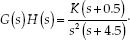 .
. - Sketch the root locus of the system whose loop transfer function is given by
 .
. - Sketch the root locus of the system whose loop transfer function is given by

- 52. Construct the root locus of the system whose loop transfer function is given by


