
14
MATLAB PROGRAMS
14.1 Introduction
MATLAB stands for MATrixLABoratory. It is a technical computing environment for high-performance numeric computation and visualization. It integrates numerical analysis, matrix computation, signal processing and graphics in an easy-to-use environment, where problems and solutions are mathematically expressed instead of traditional programming. MATLAB allows us to express the entire algorithm in a few dozen lines, to compute the solution with great accuracy in a few minutes on a computer and to readily manipulate a three-dimensional display of the result in colour.
MATLAB is an interactive system whose basic data element is a matrix that does not require dimensioning. It enables us to solve many numerical problems in a fraction of the time than it would take to write a program and execute in a language such as FORTRAN, BASIC or C. It also features a family of application-specific solutions called toolboxes. Areas in which toolboxes are available include control system design, image processing, signal processing, dynamic system simulation, system identification, neural networks, wavelength communication and others. It can handle linear, non-linear, continuous-time, discrete-time, multivariable and multirate systems. This chapter gives simple programmes to solve specific problems that are included in the previous chapters.
The system models in a control system which are developed by applying laws such as Kirchhoff's current law, Kirchhoff's voltage law, Newton's laws and so on lead to linear, non-linear and ordinary differential equations. The standard input signals are applied to the system model to obtain the response of a control system. The compensation system are used along with the system to improve and optimize the system if the response of the system is unsatisfactory.
There exists two approach for the analysis and design of control systems. They are classical or frequency domain approach and state−variable approach. In classical approach, differential or difference equations are converted into transfer functions by relating the input and output using Laplace or z-transforms and then the transfer functions are used for analysing the system.
14.2 MATLAB in Control Systems
14.2.1 Laplace Transform
Laplace transform converts the differential equations of a dynamic system into algebraic equations of a complex variable s. The syntax for using the Laplace transform in MATLAB is laplace(function_in_time_domain).
The commands which are to be used in getting the Laplace transform of a system are:
syms t
f = function_in_t
laplace(f)
14.2.2 Inverse Laplace Transform
The inverse Laplace transform helps in determining the system equations in time domain t from the equations in s domain. The syntax for using the inverse Laplace transform in MATLAB is
ilaplace(function_in_s_domain).
The commands which are to be used in getting the system equation in time domain are:
syms s,t
f = function_in_s
ilaplace(f)
Example for the usage of laplace and ilaplace command is given in Table 14.1
Table 14.1 ∣ Laplace and inverse Laplace transform in MATLAB

14.2.3 Partial Fraction Expansion
Let us consider a polynomial  where
where ![]() and
and ![]() are coefficients of
are coefficients of ![]() in the numerator and denominator respectively. The above polynomial can be simplified using partial fraction expansion that is a tedious process. MATLAB provides a simplified way for converting a polynomial into a partial fractions. The command in MATLAB for partial fraction conversion is residue (numerator, denominator).
in the numerator and denominator respectively. The above polynomial can be simplified using partial fraction expansion that is a tedious process. MATLAB provides a simplified way for converting a polynomial into a partial fractions. The command in MATLAB for partial fraction conversion is residue (numerator, denominator).
The commands which are to used in getting the partial fraction of a polynomial is given below:
n = [bm bm−1 … b1 b0] % coefficients of numerator polynomial
d = [an an−1 … a1 a0] % coefficients of denominator polynomial
[r, p, k] = residue (n, d)
where r is the column vector that contains the residues, p is the column vector that contains the poles of the system and k is the row vector which contains the direct terms.
Therefore, the partial fraction of the ![]() is
is

If all the values in the column vector ![]() are same, then
are same, then

Example for the usage of residue command is given in Table 14.2.
Consider a polynomial 
Table 14.2 ∣ Partial fraction in MATLAB

Therefore, 
Similarly, to obtain polynomials of the numerator and the denominator, we can use the same residue command as follows:
[n, d] = residue(r, p, k)
Example for the usage of residue command for getting the coefficients of polynomial is given in Table 14.3.
Table 14.3 ∣ Usage of residue command in MATLAB

14.2.4 Transfer Function Representation
The time-domain analysis, frequency domain analysis and stability of the system can be analysed easily when the model of the system is represented in the form of transfer function. Let the transfer function of a system be
![]()
The above transfer function can be represented in MATLAB, if the coefficients of numerator polynomial and denominator polynomial are known. These coefficients are known by taking the Laplace transform of the equation in time domain which has been explained in the previous section.
Consider the transfer function of a system be
![]()
In MATLAB, this transfer function can be represented using the following syntax:
n = [bm bm−1 … b1 b0]
d = [an an−1 … a1 a0]
sys = tf (n, d)
Similarly, if the transfer function of the system is obtained in MATLAB, the coefficients of the numerator and denominator polynomials can be obtained using the command tfdata.
The syntax for using the command tfdata is
[n, d] = tfdata(sytem_transfer_function, 'v')
where the variable v ensures that the output variables n and d are polynomials of transfer function and return the values as a row vector. The usage of commands tf and tfdata for getting the transfer function of a system and getting the coefficients of the polynomial is given in Table 14.4.
Table 14.4 ∣ Usage of tf and tfdata commands in MATLAB

14.2.5 Zeros and Poles of a Transfer Function
The gain, zeros and poles of a transfer function can be obtained in MATLAB using the command tf2zp. The syntax for using the command is
[z, p, k] = tf2zp (numerator_poly, denominator_poly)
where z is the zeros of the transfer function, p is the poles of the transfer function and k is the gain of the system.
Example for the usage of tf2zp for getting the gain, zeros and poles of a transfer function is given in Table 14.5.
Table 14.5 ∣ Zeros and poles from a transfer function in MATLAB

Also, from the poles, zeros and gain of a system, the coefficients of the polynomial of a transfer function can be obtained using the command zp2tf. The syntax for using the command is
[n, d] = zp2tf (z, p, k)
Example for the usage of zp2tf for getting the coefficients of polynomial of a transfer function is given in Table 14.6.
Table 14.6 ∣ Coefficients of polynomial from zeros and poles of a system

The command printsys used in the above code will be help in printing the transfer function of the system as a ratio of two polynomials in the variable mentioned within the quotes.
It is to be noted that if the commands tf2zp and zp2tf are used alone (i.e., without any output variable), the output will show only the zeros and coefficient of the numerator polynomial respectively. An example to explain the above concept is given in Table 14.7.
Table 14.7 ∣ Usage of tf2zp and zp2tf in MATLAB

14.2.6 Pole-Zero Map of a Transfer Function
The poles and zeros of a transfer function can be plotted in a graph in MATLAB using the command pzmap. The syntax for using the command is
pzmap(n, d)
Example for the usage of pzmap for plotting the poles and zeros of a transfer function is given in Table 14.8.
Table 14.8 ∣ Pole-zero map in MATLAB

14.2.7 State-Space Representation of a Dynamic System
The state-space representation of a continuous dynamic system is described by
![]()
![]()
where ![]() is the velocity vector or the derivative of the state vector of order (n × 1)
is the velocity vector or the derivative of the state vector of order (n × 1)
![]() is the state vector of order (n × 1)
is the state vector of order (n × 1)
![]() is the input or control signal vector of order (m × 1)
is the input or control signal vector of order (m × 1)
![]() is the output vector of order (p × 1)
is the output vector of order (p × 1)
![]() is the system or state matrix of order (n × n)
is the system or state matrix of order (n × n)
![]() is the input matrix of order (n × m)
is the input matrix of order (n × m)
![]() is the output matrix of order (p × n)
is the output matrix of order (p × n)
![]() is the feed-through or feed-forward matrix of order (p × m)
is the feed-through or feed-forward matrix of order (p × m)
If the matrices A, B, C and D are known, these matrices can be converted into a state-space model in MATLAB with the help of the command ss. The syntax for using the command is
variable_name = ss (A, B, C, D)
Example for the usage of ss for creating the state-space model for a system is given in Table 14.9.
Table 14.9 ∣ Creation of state-space model for a system

14.2.8 Phase Variable Canonical Form
The phase variable canonical form of a system can be obtained from the state-space model of a system using the similarity transformation matrix P such that

where ![]() and
and ![]() are the system matrices in phase variable canonical form.
are the system matrices in phase variable canonical form.
Consider a state-space matrices of a system as  ,
,  ,
, ![]() and
and ![]() . Obtain the phase variable canonical form of the system using MATLAB with the help of the similarity transformation matrix
. Obtain the phase variable canonical form of the system using MATLAB with the help of the similarity transformation matrix  .
.
The code which is used for determining the phase variable canonical form of a system is given below:

14.2.9 Transfer Function to State-Space Conversion
The transfer function of a system can be converted into a state-space model using the command tf2ss. The syntax for using the command is
[A, B, C, D] = tf2ss (n, d)
where n is the row vector that contains the coefficient of numerator polynomial and d is the row vector which contains the coefficient of denominator polynomial
14.2.10 State-Space to Transfer Function Conversion
The state-space model of a system can be converted into a transfer function model using the command ss2tf. The syntax for using the command is
[n, d] = ss2tf (A, B, C, D, k)
where the parameter k is required if the system has more than one input and the value of k specifies the particular input.
An example for the usage of ss2tf to obtain transfer function of a system whose state-space model is given by  ,
,  ,
, ![]() and
and ![]() and the usage of tf2ss to obtain state-space model of a system whose transfer function is given by
and the usage of tf2ss to obtain state-space model of a system whose transfer function is given by  is given in Table 14.10.
Table 14.10 ∣ Usage of tf2ss and ss2tf in MATLAB for a system

14.2.11 Series/Cascade, Parallel and Feedback Connections
If there exists two transfer functions ![]() and
and ![]() which are connected either in series (cascade), parallel or in feedback connection as given in Table 14.11, the resultant transfer function of the system in MATLAB is obtained using the functions mentioned below.
which are connected either in series (cascade), parallel or in feedback connection as given in Table 14.11, the resultant transfer function of the system in MATLAB is obtained using the functions mentioned below.
Consider two systems with the transfer functions ![]() and
and ![]()
where ![]() are the row matrices that contain the coefficients of numerator polynomials of transfer function
are the row matrices that contain the coefficients of numerator polynomials of transfer function ![]() and
and ![]() respectively and
respectively and ![]() are the row matrices that contain the coefficients of denominator polynomials of transfer function
are the row matrices that contain the coefficients of denominator polynomials of transfer function ![]() and
and ![]() respectively.
respectively.
The syntax for determining the resultant of the system for different type of connection is given in Table 14.11.
Table 14.11 ∣ Syntax for Series, Parallel and Cascade connections in MATLAB

where ![]() and
and ![]() are the row matrices which contains the coefficients of numerator polynomials of series, parallel and feedback connection respectively.
are the row matrices which contains the coefficients of numerator polynomials of series, parallel and feedback connection respectively. ![]() and
and ![]() are the row matrices which contains the coefficients of numerator polynomials of series, parallel and feedback connection respectively.
are the row matrices which contains the coefficients of numerator polynomials of series, parallel and feedback connection respectively.
An example to explain the concept of series, parallel and feedback connection is given in Table 14.12.
Table 14.12 ∣ Series, parallel and feedback connections using MATLAB

14.2.12 Time Response of Control System
The detailed study about the time-domain analysis of a system is described in Chapter 5. In this section, we will be discussing how the time-domain analysis can be analysed using MATLAB.
14.2.12.1 Step response of a system:
The step response of a system can be obtained if the system is represented either by state-space model or transfer function model. The different syntax for determining the step response of a systems are given below:
Case 1: If the system is described using the transfer function:
- step (n, d): This function will plot the time response of the system based on the default values of time t.
- step (n, d, t): This function will plot the time response of the system based on the user-defined values of time t.
Examples for using the command is given in Table 14.13.
Case 2: If the system is described using state-space model:
- step (A, B, C, D): This function will plot the time response of the system based on the default values of time t.
- step (A, B, C, D, 1, t): This function will plot the time response of the system based on the user defined values of time t.
- step (A, B, C, D, i, t): This function will plot the time response of the multi-input−multi-output (MIMO) system based on the input specified by i for the user defined values of time t.
Table 14.13 ∣ Step response from transfer function

If i = 0 for the MIMO system, the number of time response graphs which will be displayed is (n * n) where n is the number of input to the system or number of output from the system.
Example for using the command is given in Table 14.14.
Table 14.14 ∣ Step response from state-space model

In addition, the step response of the system can be obtained using the plot command for a system when it is represented either by means of transfer function or by state-space model. The syntax for the usage of plot command given below:
Case 1: If the system is described by the transfer function
- [y, x, t] = step (n, d); (based on the default values of time t)
plot (t, y)
- [y, x, t] = step (n, d, t); (based on the user defined values of time t)
plot (t, y)
Case 2: If the system is described by the state-space model
- [y, x, t] = step (A, B, C, D); (based on the default values of time t)
plot (t, y)
- [y, x, t] = step (A, B, C, D, 1, t); (based on the user defined values of time t)
plot (t, y)
- MIMO system
- Based on the default values of time t
- [y, x, t] = step (A, B, C, D); (when i = 0)
plot (t, y)
- [y, x, t] = step (A, B, C, D, i); (when i > 0)
plot (t, y)
- [y, x, t] = step (A, B, C, D); (when i = 0)
- Based on the user defined values of time t
(c) [y, x, t] = step (A, B, C, D, i, t); (when i > 0)
plot (t, y)
An example to show the usage of plot command in plotting the time response of the system is given in Table 14.15.
Table 14.15 ∣ Step response of a system using plot command

14.2.12.2 Impulse Response of a System: The different MATLAB commands used for determining the time response of a system when a system is subjected to impulse input is given in Table 14.16.
Table 14.16 ∣ Impulse response of a system in MATLAB

14.2.12.3 Ramp Response of a System: Similar to the step and impulse response of a system, it is not so easy to determine the ramp response of a system as ramp command does not exists in MATLAB. But by using the default command such as step and impulse it is possible to determine the ramp response of a system.
- With the help of step command: If the transfer function of the system is divided by s, then the step command can be used to determine the time response of the system when it is subjected to ramp input.
An example to determine the ramp response of a system using the step command is given in Table 14.17.
- With the help of impulse command
If the transfer function of the system is divided by s2, then the impulse command can be used to determine the time response of the system when it is subjected to ramp input.
Table 14.17 ∣ Ramp response of a system using step command in MATLAB

An example to determine the ramp response of a system using the impulse command is given in Table 14.18.
Table 14.18 ∣ Ramp response of a system using impulse command in MATLAB

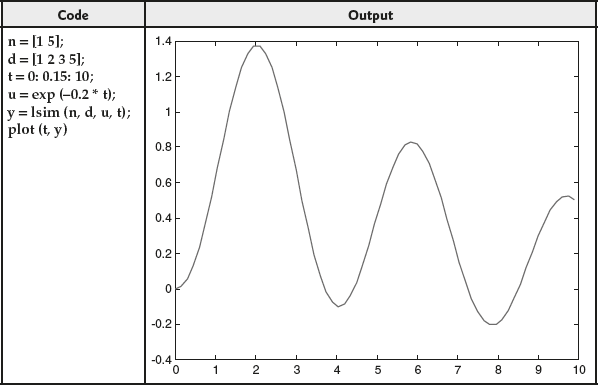
14.2.12.4 Response to an Arbitrary Input: The MATLAB command lsim is used to determine the time response of a system when the system is subjected to any random input other than the standard inputs. The main difference between the other commands (step, impulse) is that the time values should be mentioned in lsim command. The different syntax used for determining the time response of a system when it is subjected to an input u is given below:
- When a system is represented in the form of transfer function
- lsim (n, d, u, t)
- y = lsim (n, d, u, t)
plot (t, y)
- When a system is represented in the form of state-space model
- lsim (A, B, C, D, u, t): when a system is represented in the form of state-space model
- y = lsim (A, B, C, D, u, t)
plot (t, y)
An example for the usage of lsim command in MATLAB is given in Table 14.19.
Table 14.19 ∣ Response of a system for an arbitrary input
14.2.13 Performance Indices from the Response of a System
The different performance indices which can be obtained from the time response of a system are
- Delay time

- Rise time

- Peak time

- Maximum peak overshoot

- Settling time

As the formulae for determining the performance indices varies for different inputs, it is necessary to write individual programmes for different inputs. But if the formulae are not used to determine the performance indices, a single programme will be enough to determine the performance indices for all the inputs.
A programme to determine the performance indices of a system for Step input is given in Table 14.20.
Table 14.20 ∣ Code to determine the performance indices of a system
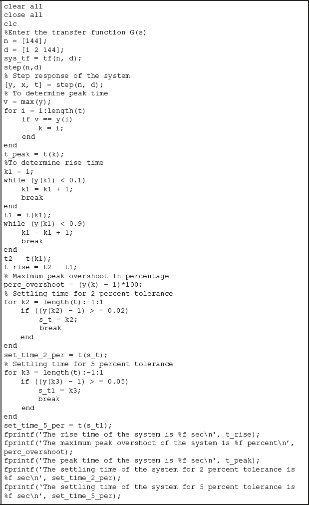
The output of the code given in Table 14.20 is given in Table 14.21.
Table 14.21 ∣ Output of the code

14.2.14 Steady State Error from the Transfer Function of a System
The steady-state error of a system is determined with the help of the error constants (position, velocity and acceleration error constants). In addition, the steady-state error and the error constants depends on both TYPE of the system and type of the input applied to the system.
The relationship among the TYPE of the system, static error constant and steady-state error of the system is given in Table 5.5.
A program to determine the steady-state error of a system for any input and any TYPE of a system is given in Table 14.22
Table 14.22 ∣ Code to determine the steady-state error of a system

The output for the code given in Table 14.22 is given below:
The given system is Type 2 system
The error constants of the system are
Kp = Inf
Kv = Inf
Ka = 1.666667
The steady state error of the system for
Unit step input = 0.000000
Unit ramp input = 0.000000
Unit parabolic input = 0.600000
14.2.15 Routh−Hurwitz Criterion
The Routh−Hurwitz criterion is one of the method for determining the stability of the system. The characteristic equation of a system is to be known for determining the stability of a system based on Routh−Hurwitz criterion. The detailed description about the Routh−Hurwitz criterion is discussed in Chapter 6. A programme to determine the stability of a system based on Routh−Hurwitz criterion can be coded.
14.2.16 Root Locus Technique
The root locus technique helps in determining the stability of the system based on the location of closed-loop poles in the s-plane. The step-by-step procedure for plotting the root locus of a system is explained in Chapter 7. In MATLAB, two default command exist in plotting the root locus of a system.
Case 1: Using the command rlocus
The default command rlocus is used to plot the root locus of a system. The syntax for the command rlocus is given below:
rlocus (n, d)
where n is the row vector which contains the coefficient of numerator polynomial and d is the row vector which contains the coefficient of denominator polynomial
An example to show the usage of rlocus command in MATLAB is given in Table 14.23.
Table 14.23 ∣ Root locus of a system

In the above command, the value of gain K is automatically taken from 0 to ![]() . But if the user defines certain value of gain K, the command to be used in MATLAB for plotting the root locus of a system is
. But if the user defines certain value of gain K, the command to be used in MATLAB for plotting the root locus of a system is
rlocus (n, d, K)
where K is the user-defined values of gain K.
Case 2: Using the command plot
The plot command can also be used to plot the root locus of a system. The syntax for using the plot command are given below:
- For default gain values K:
[r, K] = rlocus (n, d);
plot (r)
- For user defined gain values K:
[r, K] = rlocus (n, d, K);
plot (r)
- r = rlocus (n, d) or
r = rlocus (n, d, K);
plot (r)
An example to show the usage of plot command to plot the root locus of a system is given in Table 14.24.
Table 14.24 ∣ Root locus of a system

It is to be noted that if a point is clicked in the root locus plot of a system, it will display the information such as frequency (rad/s), overshoot (%), damping and gain at that point.
14.2.16.1 Determination of Gain Value K at a Given Point in the Root Locus
The gain value K at any point on the root locus of a system in MATLAB is determined using the command rlocfind. The different syntax for using the command rlocfind are given below:
- [K, r] = rlocfind (n, d)
- K = rlocfind (n, d)
- rlocfind (n, d)
where K is the gain value at a particular point and r is the column vector that gives the location of roots at gain K.
In the commands shown above, the first will return both the gain and location of roots while the second and third command when used in MATLAB, will return only the gain value K.
The step-by-step procedure to determine the gain value K at a given point are given below:
- Plot the root locus of a system using the command mentioned earlier.
- Use the command rlocfind in any one of the format mentioned above.
- Once the command rlocfind is executed a message 'select a point in the figure window' will be displayed in the command window.
- A cursor will be also available in root locus plot to select an exact point in the plot.
- If we select a point in the root locus plot using the cursor, the gain and the roots at that particular point will be displayed in the command window.
An example to determine the value of gain K from the root locus using MATLAB is given in Table 14.25.
Table 14.25 ∣ Gain of a system from root locus in MATLAB

14.2.16.2 Root Locus Plot Using State-Space Representation of a System
The root locus plot for a system which is represented using the state-space model can be plotted with the help of the command rlocus. The syntax for using the command are given below:
- rlocus (A, B, C, D): gain value K ranging from 0 to

- rlocus (A, B, C, D, K): user-defined values of gain K
Usage of plot command
- [r, K] = rlocus (A, B, C, D) − gain value K ranging from 0 to

plot (r)
- [r, K] = rlocus (A, B, C, D, K) user-defined values of gain K
plot (r)
An example to show the usage of rlocus plot using state-space model is given in Table 14.26.
Table 14.26 ∣ Root locus of a state − space model of a system

14.2.17 Bode Plot
The Bode plot is one of the frequency-response technique which is used to analyse the stability of the system. The stability of the system is analysed based on the value of the frequency domain specifications (gain margin, phase margin, gain crossover frequency and phase crossover frequency). The manual determination of frequency domain specification from the Bode plot is discussed in Chapter 8. In this section, plotting of Bode plot in MATLAB and determination of frequency domain specification from Bode plot in MATLAB are discussed.
Plotting Bode plot for system
The default command in MATLAB which is used for plotting the Bode plot of a system is bode. The syntax for using the command bode for plotting the Bode plot for a system are given below:
Case A: If the system is represented in the transfer function model
- If the frequency range for plotting the Bode plot is automatically selected, the syntax for plotting the Bode plot will be
bode (n, d) or
bode (sys_tf)
where n is the row vector containing the coefficients of numerator polynomial, d is the row vector containing the coefficients of denominator polynomial and sys_tf is the system transfer function obtained using the command tf.
An example for plotting the Bode plot is given in Table 14.27.
Table 14.27 ∣ Bode plot of a system

- If the frequency range for plotting the Bode plot is user defined, the syntax for plotting the Bode plot will be
bode (n, d, w) or
bode (sys_tf, w)
where w is the range of frequency for plotting the Bode plot.
As the Bode plot is plotted in the logarithmic scale of the frequency w the user-defined values should also be in logarithmic scale. The MATLAB command which is used to obtain the frequency value in logarithmic scale is
w = logspace (a, b).
where 10a is the starting point of frequency range and 10b is the ending point of frequency range
An example for plotting the Bode plot is given in Table 14.28.
Table 14.28 ∣ Bode plot of a system

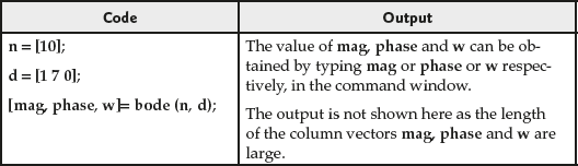
- When the magnitude and phase values corresponding to different frequencies are to be stored, the syntax for getting the values will be
- For default values of frequency w
[mag, phase, w] = bode (n, d) or
[mag, phase, w] = bode (sys_tf)
- For user defined values of frequency w
[mag, phase, w] = bode (n, d, w) or
[mag, phase, w] = bode (sys_tf, w)
where mag and phase are the column vectors that contains the magnitude and phase values of the system corresponding to the different frequencies respectively.
Here, mag value can be converted into decibels with the help of 20 *log10(mag).
An example for obtaining the magnitude and phase values corresponding to different frequencies is given in Table 14.29.
Table 14.29 ∣ Bode plot of a system
It is to be noted that at a particular frequency, the magnitude and phase angles can be obtained by clicking at the plot which is shown in Fig. 14.1.
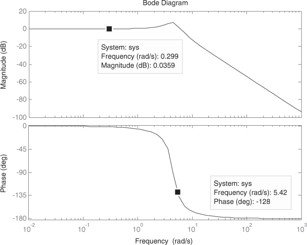
Fig. 14.1 ∣ Bode plot with the magnitude and phase angle at a frequency
- For default values of frequency w
14.2.17.1 Determination of frequency domain specification from Bode plot
The frequency domain specifications which can be obtained from Bode plot are gain margin, phase margin, gain crossover frequency and phase crossover frequency. The definition of each frequency domain specifications and its manual calculation is discussed in Chapter 8. In this section, determination of frequency domain specification values from Bode plot using MATLAB is discussed.
The default command used in MATLAB for determining the frequency domain specification is margin. The syntax for using the command in MATLAB are given below:
- margin (n, d) displays only the gain margin and phase margin of the system.
or [Gm, Pm, pcf, gcf] = margin (n, d) displays all the frequency domain specifications.
- margin (sys_tf) displays only the gain margin and phase margin of the system.
or [Gm, Pm, pcf, gcf] = margin (sys_tf) displays all the frequency domain specifications.
where Gm is the gain margin of the system, Pm is the phase margin of the system, pcf is the phase crossover frequency of the system and gcf is the gain crossover frequency of the system.
An example to show the usage of the command is given in Table 14.30.
Table 14.30 ∣ Frequency domain specification of a system using bode plot

Case B: If the system is represented using state-space model
- System with one input
- If the frequency range for plotting the Bode plot is automatically selected, the syntax for plotting the Bode plot will be
bode (A, B, C, D)
where A, B, C, D are the state-space matrix of a system.
- If the frequency range for plotting the Bode plot is user defined, the syntax for plotting the Bode plot will be
bode (A, B, C, D, 1, w)
where w is the user-defined frequency range obtained using the default command logspace.
An example for the usage of the command bode is given in Table 14.31.
Table 14.31 ∣ Bode plot of a system

- If the frequency range for plotting the Bode plot is automatically selected, the syntax for plotting the Bode plot will be
- System with more than one input and more than one output.
- If the input to which the Bode plot is to be plotted is mentioned. The syntax will be
bode (A, B, C, D, i)
where i is the input for which the Bode plot has to be plotted.
- If the input to which the Bode plot is to be plotted is not mentioned. The syntax will be
bode (A, B, C, D)
If we use this command, the number of bode plots generated will be

where m is the number of inputs and n is the number of outputs.
If the system has two inputs and two outputs, then the number of Bode plot generated by using the second command will be 4 (2 * 2).
An example for the usage of this command is given in Table 14.32.
- If the frequency range for plotting the Bode plot is user defined, the syntax for plotting the Bode plot will be
bode (A, B, C, D, i, w)
- If the input to which the Bode plot is to be plotted is mentioned. The syntax will be
Table 14.32 ∣ Bode plot of a system

An example for the usage of this command is given in Table 14.33.
Table 14.33 ∣ Bode plot of a system

It is to be noted that the determination of frequency domain specification using the default command margin in MATLAB is not possible. To use the default command margin, the system must be a SISO system.
14.2.18 Nyquist Plot
The frequency response technique that analyze the stability of the closed-loop system based on the open-loop frequency response is known as Nyquist plot. The detailed analysis of the Nyquist plot is discussed in Chapter 9. The default command which is used to plot the Nyquist plot of a system in MATLAB is nyquist. The syntax for using the command in MATLAB are discussed below for different cases.
Case A: If the system is represented in the transfer function model
- If the frequency range for plotting the Nyquist plot is automatically selected, the syntax for plotting the Nyquist plot will be
nyquist (n, d) or
nyquist (sys_tf)
where n is the row vector containing the coefficients of numerator polynomial, d is the row vector containing the coefficients of denominator polynomial and sys_tf is the system transfer function obtained using the command tf.
- If the frequency range for plotting the Nyquist plot is user defined, the syntax for plotting the Nyquist plot will be
nyquist (n, d, w) or
nyquist (sys_tf, w)
where w is the range of frequency for plotting the Nyquist plot.
The range of frequency is generated with the help of the command linspace. The syntax for usage of linspace is
w = linspace (a, b, c);
where a is the starting point of the frequency range, b is the ending point of the frequency range and c is the number of points to be taken between a and b.
An example for plotting the Nyquist plot is given in Table 14.34.
- When the real and imaginary values corresponding to different frequencies are to be stored, the syntax for getting the values will be
- For default values of frequency w
[re, im, w] = nyquist (n, d) or
[re, im, w] = nyquist (sys_tf)
- For user defined values of frequency, w
[re, im, w] = nyquist (n, d, w) or
[re, im, w] = nyquist (sys_tf, w)
where re and im are the column vectors that contain the real and imaginary values of the system corresponding to the different frequencies respectively.
- For default values of frequency w
An example for obtaining the real and imaginary values corresponding to different frequencies is given in Table 14.35.
Table 14.34 ∣ Nyquist plot of a system

Table 14.35 ∣ Nyquist plot data of a system

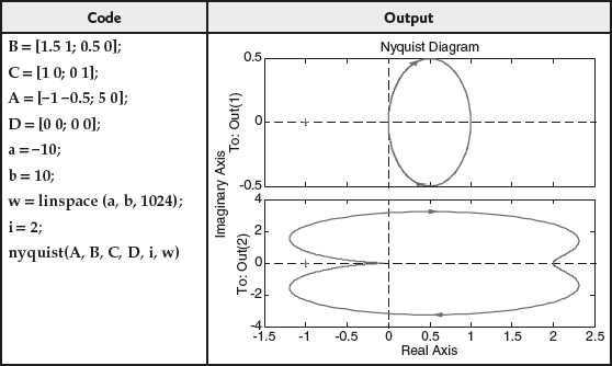
It is to be noted that at a particular frequency, the real value, imaginary value and its corresponding frequency can be obtained by clicking at the plot which is shown in Fig. 14.2.
Case B: If the system is represented using state-space model
- System with one input
- If the frequency range for plotting the Nyquist plot is automatically selected, the syntax for plotting the Nyquist plot will be
nyquist (A, B, C, D)
where A, B, C, D are the state-space matrix of a system.
- If the frequency range for plotting the Nyquist plot is user defined, the syntax for plotting the Nyquist plot will be
nyquist (A, B, C, D, 1, w)
where w is the user-defined frequency range obtained using the default command logspace.

Fig. 14.2 ∣ Nyquist plot with the real and imaginary value at a frequency
An example for the usage of the command nyquist is given in Table 14.36
Table 14.36 ∣ Nyquist plot

- If the frequency range for plotting the Nyquist plot is automatically selected, the syntax for plotting the Nyquist plot will be
- 2. System with more than one input and more than one output.
- If the frequency range for plotting the Nyquist plot is automatically selected, the syntax for plotting the Nyquist plot will be
- If the input to which the Nyquist plot of a system is to be plotted is mentioned, the syntax will be
nyquist (A, B, C, D, i)
where i is the input for which the Nyquist plot has to be plotted.
- If the input to which the Nyquist plot of a system is to be plotted is not mentioned, the syntax will be
nyquist (A, B, C, D)
If we use this command, the number of Nyquist plots generated will be
 .
.where m is the number of inputs and n is the number of outputs.
If the system has two inputs and two outputs, then the number of Nyquist plot generated by using the second command will be 4 (2 * 2).
An example for the usage of this command is given in Table 14.37.
Table 14.37 ∣ Nyquist plot for a state-space model

- If the input to which the Nyquist plot of a system is to be plotted is mentioned, the syntax will be
- If the frequency range for plotting the Bode plot is user defined, the syntax for plotting the Bode plot will be
nyquist (A, B, C, D, i, w)
An example for the usage of this command is given in Table 14.38.
- If the frequency range for plotting the Nyquist plot is automatically selected, the syntax for plotting the Nyquist plot will be
Table 14.38 ∣ Nyquist plot for state-space model with user-defined frequency
14.2.19 Design of Compensators Using Matlab
The detailed analysis of the design of compensators is discussed in Chapter 11. There is no default command which can be used for designing the compensators in MATLAB. In this section, we will be analyzing the design of compensators in MATLAB with the help of an example.
14.2.19.1 Lag compensator: Consider an uncompensated system with the open-loop transfer function as ![]() . Design a lag compensator for the system such that the compensated system has static velocity error constant
. Design a lag compensator for the system such that the compensated system has static velocity error constant ![]() , phase margin
, phase margin ![]() and the gain margin
and the gain margin ![]() .
.
Solution
As discussed in Chapter 10, step-by-step procedure are followed to determine the transfer function of the compensator.
- The value of
 is determined as 5.
 - The bode plot for the system
 is plotted and the frequency domain specifications are determined in MATLAB as given in Table 14.39.
 - Adding tolerance of
 , the desire phase margin will be
  .
. - To have the phase margin of
 , the phase angle of the system should be
  . Therefore, for
  , the frequency of the system is
  rad/s. Hence,
  =
=  rad/s.
Table 14.39 ∣ Bode plot for uncompensated system

- The magnitude value
 in dB corresponding to
  is 17.5 dB. The magnitude value from bode plot corresponding to desired phase margin is shown in Fig. 14.3.

Fig. 14.3 ∣ Magnitude value corresponding to desired phase margin
- The value of
 is determined using the formula
  and the value is determined as
  .
. - The value of
 is determined using the formula
  and the value is determined as
  .
. - Therefore, the transfer function of the lag compensator will be

- Thus, the transfer function of the compensated system will be

- The bode plot of the compensated system is plotted in MATLAB and the plot is given in Table 14.40.
Table 14.40 ∣ Bode plot of compensated system

14.2.19.2 Lead compensator: Consider an uncompensated system with the open-loop transfer function as ![]() . Design a lead compensator for the system such that the compensated system has static velocity error constant
. Design a lead compensator for the system such that the compensated system has static velocity error constant ![]() , phase margin
, phase margin ![]() and the gain margin gm = 10 dB.
and the gain margin gm = 10 dB.
Solution
As discussed in Chapter 10, step-by-step procedure are followed to determine the transfer function of the compensator.
- The value of
 is determined as 10.
 - The bode plot for the system
 is plotted and the frequency domain specifications are determined in MATLAB as given in Table 14.41.
Table 14.41 ∣ Bode plot for uncompensated system

- By adding tolerance of
 ,
,  is calculated as
  .
. - The value of
 is determined using
  and the obtained value of
  is 0.24.
 - Determine
 dB which is −6.2 dB. Let
  dB.
dB. - The frequency corresponding to
 dB is 4.48 rad/s which is determined from magnitude plot of the system as shown in Fig. 14.4. Let that frequency be
  .
. - Using the formula
 , the value of T is determined as 0.455.
 - The value of
 is determined using the formula
  as 41.66.
 - Therefore, the transfer function of the lead compensator will be


Fig. 14.4 ∣ Determination of frequency corresponding to AdB
- Thus, the transfer function of the compensated system will be

- The bode plot of the compensated system is plotted in MATLAB and the plot is given in Table 14.42.
14.2.19.3 Lag–Lead compensator: Consider an uncompensated system with the open-loop transfer function as ![]() . Design a lag−lead compensator for the system such that the compensated system has static velocity error constant
. Design a lag−lead compensator for the system such that the compensated system has static velocity error constant ![]() , phase margin
, phase margin ![]() and the gain margin
and the gain margin ![]() .
.
Solution
As discussed in Chapter 10, step-by-step procedure are followed to determine the transfer function of the compensator.
- The value of
 is determined as 20.
 - The bode plot for the system
 is plotted and the frequency domain specifications are determined in MATLAB as given in Table 14.43.
Table 14.42 ∣ Bode plot of compensated system
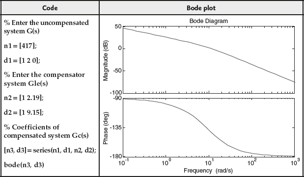
Table 14.43 ∣ Bode plot for uncompensated system

- Let

- Using the formulae
 and
and  , the value of
  is determined as 7.54.
 - Let
 rad/s.
 - The time constant of lag compensator is determined as:
 rad/s.
 - Therefore, the transfer function of lag compensator is
 .
. - The magnitude of the system from the magnitude plot at
 dB. The determination of magnitude of the system from magnitude plot is shown in Fig. 14.5.
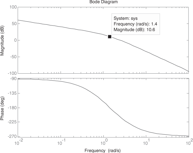
Fig. 14.5 ∣ Determination of magnitude A at

- If the slope of +20 dB/decade is drawn from (1.4 rad/s, −10.7 dB), the slope cuts the 0dB line and −20 dB line at
 rad/s and at
  rad/s respectively.
 - Thus, the transfer function of the lead portion of the lag−lead compensator is

- Therefore, the transfer function of the lag−lead compensator is

- Thus, the transfer function of the compensated system is

- The bode plot of the compensated system is plotted in MATLAB and the plot is given in Table 14.44.
Table 14.44 ∣ Bode plot of compensated system
