1.1 Introduction
A system is a combination of components connected to perform a required action. The control component of a system plays a major role in altering or maintaining the system output based on our desired characteristics. There are two types of control systems: manual control and automatic control. For example, in manual control, a man can switch on or switch off the bore well motor to control the level of water in a tank. On the other hand, in automatic control, level switches and transducers are used to control the level of water in a tank.
Control systems have naturally evolved in our ecosystem. In almost all living things, automatic control regulates the conditions necessary for life by tackling the disturbance through sensing and controlling functionalities. They operate complex systems and processes and achieve control with desired precision. The application of control systems facilitates automated manufacturing processes, accurate positioning and effective control of machine tools. They guide and control space vehicles, aircrafts, ships and high-speed ground transportation systems. Modern automation of a plant involves components such as sensors, instruments, computers and application of techniques that involve data processing and control.
It is essential to understand a system and its characteristics with the help of a model, before creating a control for it. The process of developing a model is known as modeling. Physical systems are modeled by applying notable laws that govern their behaviour. For example, mechanical systems are described by Newton's laws and electrical systems are described by Ohm's law, Kirchhoff's law, Faraday's and Lenz's law. These laws form the basis for the constitutive properties of the elements in a system.
1.2 Classification of Control System
Control systems are generally classified as (i) open-loop control systems and (ii) closed-loop control systems as shown in Fig. 1.1.

Fig. 1.1 ∣ Classification of control systems
1.2.1 Open-Loop Control System
A control system that cannot adjust itself to the changes is called open-loop control system. In general, manual control systems are open-loop systems. The block diagram of open-loop control system is shown in Fig.1.2.
Fig. 1.2 ∣ Block diagram of an open-loop control system
Here, ![]() is the input signal,
is the input signal, ![]() is the control signal/actuating signal and
is the control signal/actuating signal and ![]() is the output signal.
is the output signal.
In this system, the output remains unaltered for a constant input. In case of any discrepancy, the input should be manually changed by an operator. An open-loop control system is suited when there is tolerance for fluctuation in the system and when the system parameter variation can be handled irrespective of the environmental conditions.
In olden days, air conditioners were fitted with regulators that were manually controlled to maintain the desired temperature. This real-time system serves as an open-loop control system as shown in Fig.1.3.
Fig. 1.3 ∣ Open-loop control system of an air conditioner
1.2.2 Closed-Loop Control System
Any system that can respond to the changes and make corrections by itself is known as closed-loop control system. The only difference between open-loop and closed-loop systems is the feedback action. The block diagram of a closed-loop control system is shown in Fig.1.4.

Fig. 1.4 ∣ Block diagram of closed-loop control system
Here, ![]() is the input signal,
is the input signal, ![]() is the error signal/actuating signal,
is the error signal/actuating signal, ![]() or m(t) is the control signal/manipulated signal, b(t) is the feedback signal and
or m(t) is the control signal/manipulated signal, b(t) is the feedback signal and ![]() is the controlled output.
is the controlled output.
Here, the output of the machine is fed back to a comparator (error detector). The output signal is compared with the reference input ![]() and the error signal
and the error signal ![]() is sent to the controller. Based on the error, the controller adjusts the air conditioners input [control signal
is sent to the controller. Based on the error, the controller adjusts the air conditioners input [control signal ![]() ]. This process is continued till the error gets nullified. Both manual and automatic controls can be implemented in a closed-loop system. The overall gain of a system is reduced due to the presence of feedback. In order to compensate for the reduction of gain, if an amplifier is introduced to increase the gain of a system, the system may sometimes become unstable.
]. This process is continued till the error gets nullified. Both manual and automatic controls can be implemented in a closed-loop system. The overall gain of a system is reduced due to the presence of feedback. In order to compensate for the reduction of gain, if an amplifier is introduced to increase the gain of a system, the system may sometimes become unstable.
Present-day air conditioners are designed with temperature sensors, comparators and controller modules. The reference temperature (the desired room temperature) is fed and compared with actual room temperature, which is sensed by a temperature sensor. The difference between these two values, i.e., the error signal is fed to a controller and the controller performs the necessary action to minimize the error. The block diagram for this example is shown in Fig.1.5.

Fig. 1.5 ∣ Closed-loop control system of an air conditioner
A person driving a car is also an example for a closed-loop control system as shown in Fig.1.6. During the ride, the brain controls the hands for steering, gear, horn and the legs for brake and accelerator so as to perform the driving in a perfect manner. The eyes and the ears form the feedback, i.e., eyes for determining the pathway and mirror view and ears for sensing other vehicles nearby. The driver also accelerates or decelerates depending on the terrain and traffic involved.
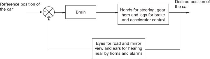
Fig. 1.6 ∣ Closed-loop system of a driver controlled car
1.3 Comparison of Open-Loop and Closed-Loop Control Systems
Table 1.1 discusses the comparison of open-loop and closed-loop control systems.
Table 1.1 ∣ Comparison of open-loop and closed-loop control systems

1.4 Differential Equations and Transfer Functions
For the analysis and design of a system, a mathematical model that describes its behaviour is required. The process of obtaining the mathematical description of a system is known as modeling. The differential equations for a given system are obtained by applying appropriate laws, for example, Newton's laws for mechanical systems and Kirchhoff's law for electrical systems. These equations may be either linear or non-linear based on the system being modeled. Therefore, deriving appropriate mathematical models is the most important part of the analysis of a system.
A system is said to be linear if it obeys the principles of superposition and homogeneity. If a system has responses ![]() and
and ![]() for any two inputs
for any two inputs ![]() and
and ![]() respectively, then the system response to the linear combination of these inputs
respectively, then the system response to the linear combination of these inputs ![]() is given by the linear combination of the individual outputs
is given by the linear combination of the individual outputs ![]() , where
, where ![]() and
and ![]() are constants. The principle of homogeneity and superposition is explained in Fig. 1.7.
are constants. The principle of homogeneity and superposition is explained in Fig. 1.7.

Fig. 1.7 ∣ Principle of homogeneity and superposition
If the coefficients of the differential equations are functions of time (an independent variable), then a system is called linear time-varying system. On the other hand, if the coefficients of the differential equations are not a function of time, then a system is called linear time-invariant system. For the transient-response or frequency-response analysis of single-input and single-output linear time-invariant system, the transfer function representation will be a convenient tool. But, if a system is subjected to multi-input and multi-output, then state-space analysis will be a convenient tool.
1.4.1 Transfer Function Representation
The transfer function of a linear, time-invariant, differential equation system is given by the ratio of Laplace transform of output variable (response function) to the Laplace transform of the input variable (driving function) under the assumption that all initial conditions are zero.
Transfer function,  at zero initial conditions.
It is to be noted that non-linear systems and time-varying systems do not have transfer functions because they do not obey the principles of superposition and homogeneity. With the concept of transfer functions, it is possible to represent system dynamics by algebraic equations in ![]() domain. The highest power of
domain. The highest power of ![]() in the denominator of a transfer function is the order of the system.
in the denominator of a transfer function is the order of the system.
1.4.2 Features and Advantages of Transfer Function Representation
The following are the features and advantages of transfer function representation:
- Using transfer functions, mathematical models can be obtained and analyzed.
- Output response can be obtained for any kind of inputs.
- Stability analysis can be performed.
- The usage of Laplace transform converts complex time domain equations to simple algebraic equations, expressed with complex variable s.
- Analysis of a system is simplified due to the use of s-domain variable in the equations, rather than using time-domain variable.
1.4.3 Disadvantages of Transfer Function Representation
The following are the disadvantages of transfer function representation:
- It is not applicable to non-linear systems or time-varying systems.
- Initial conditions are neglected.
- Physical nature of a system cannot be found (i.e., whether it is mechanical or electrical or thermal system).
1.4.4 Transfer Function of an Open-Loop System
In the block diagram of a system relating its input and output as shown in Fig.1.8, there exists an input (excitation) which operates through a transfer operator called transfer function and it produces an output (response).
Fig. 1.8 ∣ Block diagram representation of an open-loop transfer function
From the block diagram representation of an open-loop transfer function, we have

where ![]() is the Laplace transform of the input variable or excitation, C(s) is the Laplace transform of the output variable or response and
is the Laplace transform of the input variable or excitation, C(s) is the Laplace transform of the output variable or response and ![]() is the transfer function.
is the transfer function.
1.4.5 Transfer Function of a Closed-Loop System
Closed-loop control systems can be classified into two categories, based on the type of feedback signal as (i) Negative feedback systems and (ii) Positive feedback systems.
(i) Negative Feedback Systems
The simplest form of a negative-feedback control system is shown in Fig. 1.9. It has one block in the forward path and one in the feedback path.

Fig. 1.9 ∣ Block diagram representation of negative feedback control system
Practically, all control systems can be reduced to this form. ![]() represents the overall gain of the blocks in the forward path,
represents the overall gain of the blocks in the forward path, ![]() is the feedback signal,
is the feedback signal, ![]() is the error signal and
is the error signal and ![]() represents the overall gain of all the blocks in the feedback path.
represents the overall gain of all the blocks in the feedback path.
The objective is to reduce this control system to a single block by determining the closed-loop transfer function (CLTF) for the negative feedback.
The following relationships can be derived from the block diagram:
Feedback signal, B(s) = output ![]() feedback path gain
feedback path gain
![]() (1.1)
(1.1)
Error signal, ![]() = input signal − feedback signal
= input signal − feedback signal
![]() =
= ![]()
Substituting Eqn. (1.1) in the above equation, we obtain
![]() (1.2)
(1.2)
Output signal, ![]()
![]() (1.3)
(1.3)
Substituting the value of the error signal, we obtain
![]()
![]()
![]()

Hence, the transfer function of the negative feedback control system is given by
 (1.4)
(1.4)
Based on the above expression, Fig. 1.9 is reduced to the simplified form as shown in Fig. 1.10.

Fig. 1.10 ∣ Reduced form of a negative feedback control system
Thus, the closed-loop transfer function is
T(s) = ![]()
![]()
Hence, the output, ![]() = closed-loop transfer function T(s)
= closed-loop transfer function T(s) ![]() input
input ![]() .
.
Observations drawn from this relationship are:
- The control system transfer function is a property of the system.
- The transfer function is dependent only on its internal structure and components.
- The transfer function is independent of the input applied to a system.
- When an input signal is applied to a closed-loop control system, an output is generated; i.e., it is dependent on the input as well as the system transfer function.
(ii) Positive Feedback Systems
If the feedback is positive, then the closed-loop transfer function can be similarly derived as
 (1.5)
(1.5)
The block diagram representing positive feedback control system is shown in Fig. 1.11.

Fig. 1.11 ∣ Block diagram representation of positive feedback control system
1.4.6 Comparison of Positive Feedback and Negative Feedback Systems
Table 1.2 discusses the comparison of characteristics between positive feedback and negative feedback systems.
Table 1.2 ∣ Characteristics of positive feedback and negative feedback systems

Example 1.1: A negative feedback system has a forward gain of 10 and feedback gain of 1. Determine the overall gain of the system.
Solution: Given the forward gain ![]() and the feedback gain
and the feedback gain ![]()
The overall gain of a closed-loop system is same as its closed-loop transfer function. For a negative feedback system, the transfer function is given by

Substituting the values of ![]() and
and ![]() , we obtain overall gain of a closed-loop system,
, we obtain overall gain of a closed-loop system,
![]() .
.
Example 1.2: A negative feedback system with a forward gain of 2 and a feedback gain of 8 is subjected to an input of 5 V. Determine the output voltage of the system.
Solution: Given the forward gain ![]() , feedback gain
, feedback gain ![]() and input
and input ![]() .
.
Output voltage for any system is given by
![]() = Transfer function of the closed-loop system
= Transfer function of the closed-loop system ![]() input
input ![]()
The transfer function of the closed-loop system with negative feedback is given by

Substituting the values of ![]() and
and ![]() , we obtain
, we obtain

Therefore, the output voltage of the given system ![]() .
.
Example 1.3: A positive feedback system was subjected to an input of 3 V. Determine the output voltage of the following sets of gains:
 ,
, 
 ,
, 
 ,
, 
 ,
, 
-
 ,
, 
-
 ,
, 
Solution: It is known that 

The output voltage ![]() for different cases can be obtained by substituting the different values of
for different cases can be obtained by substituting the different values of ![]() ,
, ![]() and
and ![]() .
.
- When
 = 1,
= 1,  = 0.75 and
  = 3 V,

- When
 and
and  ,
,

- When
 and
and 

- When
 and
and 

- When
 and
and 

- When
 and
and 

It can be noted that, the output becomes very large and approaches infinity when the loop gain approaches a value of 1, i.e., ![]() .
.
1.5 Mathematical Modeling
The process involved in modeling a system using mathematical equations, formed by the variables and constants of the system is called the mathematical modeling of a system. For example, an electrical network can be modeled using the equations formed by Kirchhoff's laws.
Fig 1.12 shows a flow chart for determining the transfer function of any system.

Fig. 1.12 ∣ Flow chart for deriving the transfer function
1.5.1 Mathematical Equations for Problem Solving
Basic Laplace transform of different functions are
![]()
![]()
![]()
Cramer's rule:
For a given pair of simultaneous equations, we have
![]()
![]()
The above equations can be written in matrix form as

Therefore,
![]()
 and
and 
![]()
where 
 and
and  .
.
1.6 Modeling of Electrical Systems
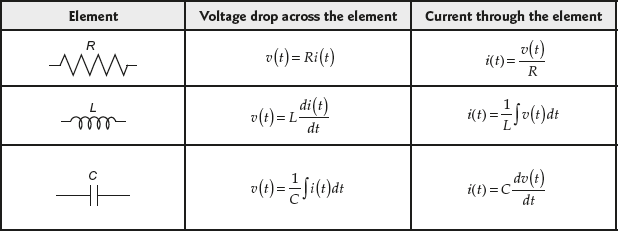
An electrical system consists of resistors, capacitors and inductors. The differential equations of electrical systems can be formed by applying Kirchhoff's laws. The transfer function can be obtained by taking Laplace transform of the integro-differential equations and rearranging them as a ratio of output to input. The relationship between voltage and current for different elements in the electrical circuit is given in Table 1.3.
Table 1.3 ∣ Relationship of voltage and current for R, L and C
Example 1.4: A rotary potentiometer is being used as an angular position transducer. It has a rotational range of 0°–300° and the corresponding output voltage is 15 V. The potentiometer is linear over the entire operating range. Determine its transfer function.
Solution: Given output voltage = 15 V and input rotation = 300°
The transfer function of the potentiometer ![]() is given by
is given by
![]()
Substituting the given values, we obtain
![]()
Example 1.5: Determine the transfer function of the electrical network shown in Fig. E1.5.

Fig. E1.5
Solution: The output voltage across the capacitor is ![]()
Applying Kirchhoff's voltage law, the loop equation is given by
![]()
Taking Laplace transform of the above equations, we obtain
![]() (1)
(1)
![]()
Simplifying the above equation, we obtain
 (2)
(2)
Substituting Eqn. (2) in Eqn. (1), we obtain

Hence, the transfer function of the system is given by

Example 1.6: Determine the transfer function of the electrical network shown in Fig. E1.6(a).

Fig. E1.6(a)
Solution: In the given circuit, there exist two impedances ![]() as shown in Fig. E1.6(b).
as shown in Fig. E1.6(b).

Fig. E1.6(b)
Therefore, ![]()
![]()
![]()
![]()
The output voltage across the impedance ![]() is
is ![]()
Applying Kirchhoff's voltage law, the loop equation is given by
![]()
Taking Laplace transform of the above equations, we obtain
![]() (1)
(1)
![]()
Simplifying, we obtain
 (2)
(2)
Substituting Eqn. (2) in Eqn. (1), we obtain

Hence, the transfer function of the system is given by

Therefore,

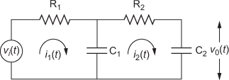
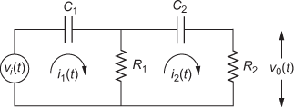
Example 1.7: Determine the transfer function of the electrical network shown in Fig. E1.7.

Fig. E1.7
Solution: The output voltage of the given electrical network is
![]()
Taking Laplace transform, we obtain
![]() (1)
(1)
The loop equations for each loop can be obtained by applying Kirchhoff's voltage law.
Loop equation for loop (1) is
![]()
Taking Laplace transform on both the sides, we obtain
 (2)
(2)
Loop equation for loop (2) is
![]()
Taking Laplace transform, we obtain
 (3)
(3)
Representing Eqn. (2) and Eqn. (3) in matrix form,

Applying Cramer's rule, we obtain
![]()
where 
and 
![]()

Therefore,

But, 

Hence, the overall transfer function of the given electrical system is given by

Example 1.8: Determine the transfer function of the electrical network shown in Fig. E1.8(a).

Fig. E1.8(a)
Solution: The above electrical network can be modified as shown in Fig. E1.8(b).

Fig. E1.8(b)
The output voltage of the given electrical circuit is
![]()
Applying Laplace transform, we obtain
![]()
 (1)
(1)
Applying Laplace transform, we obtain transformation of the parallel RC circuit as shown in Fig. E1.8(c).

Fig. E1.8(c)
Thus, the given electrical circuit is re-drawn as shown in Fig. E1.8(d).

Fig. E1.8(d)
Now, Kirchhoff's voltage law is applied to the individual loops for the above electrical circuit.
Then the equation for loop (1) is


 (2)
(2)
Loop equation for loop (2) is


 (3)
(3)
The Eqn. (2) and Eqn. (3) are written in matrix form as

Applying Cramer's rule, we obtain
![]()


 (4)
(4)
Substituting Eqn. (4) in Eqn. (1), we obtain


Thus, the overall transfer function is

1.7 Modeling of Mechanical Systems
The dimensions in which the movement of a mechanical system can be described are translational, rotational or a combination of both. For modeling of mechanical system, it is necessary to have the equations governing the movement of mechanical systems. The laws that are used directly or indirectly to formulate those equations are obtained from Newton's laws of motion.
The general classification of mechanical system is of two types: (i) translational and (ii) rotational as shown in Fig. 1.13.

Fig. 1.13 ∣ Classification of mechanical system
1.7.1 Translational Mechanical System
The modeling of linear passive translational mechanical system can be obtained by using three basic elements: mass, spring and damper. The mass that is concentrated at the center of a system is used to represent the weight of a given mechanical system, whereas the spring is used to represent the elastic deformation of the body and the damper is used to represent the friction existing in a mechanical system. An example of such linear passive translational mechanical system is the suspension system existing in the automobiles (such as car, van, etc.). For the analysis of linear passive translational mechanical system, it is assumed that the elements are purely linear.
The opposing forces due to mass, friction and spring act on a system when the system is subjected to a force. Using D'Alembert's principle, for a linear passive translational mechanical system, the sum of forces acting on a body is zero (i.e., the sum of applied forces is equal to the sum of the opposing forces on a body). Displacement, velocity and acceleration are the variables used to describe the linear passive translation mechanical system.
In translational mechanical systems, the energy storage elements are mass and spring and the element that dissipates energy is viscous damper. The analogous elements for energy storage in an electrical circuit are inductors and capacitors, whereas those of the energy dissipating element are resistors.
Inertia Force ![]()
The element that stores the kinetic energy of translational mechanical system is mass. Mass is considered to be a conservative element, as the energy can be stored and retrieved without loss.
When a force ![]() is applied to a mass M, it experiences an acceleration and it is shown in Fig. 1.14.
is applied to a mass M, it experiences an acceleration and it is shown in Fig. 1.14.
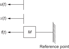
Fig. 1.14 ∣ Mass element
According to Newton's second law, the force experienced by the mass is proportional to the acceleration.
![]()
![]()
![]()
![]()
where M is the mass (kg), a is the acceleration (m/s2), ![]() is the velocity (m/s) and
is the velocity (m/s) and ![]() is the displacement (m).
is the displacement (m).
![]()
Here, ![]() is measured in Newton (N) or Kg-m/s2.
is measured in Newton (N) or Kg-m/s2.
Damper
The damping that is desirable in the motion for a mechanical system is provided by an element called damper. A frictional force that exists between one or two physical systems when there exists a movement or a tendency of movement between them. The characteristics of frictional forces that are non-linear in nature depends on the composition of the surfaces, the pressure between the surfaces, their relative velocity and others that add difficulty in obtaining the mathematical description of the frictional force. The different types of frictions that are commonly used in practical system are viscous friction, static friction and coulomb friction in which the viscous friction is commonly found in a translational mechanical system.
Static Friction or Stiction
The retarding force ![]() which tends to prevent the motion is known as static friction or stiction. This type of frictional force exists only when the body is not in motion (stationary), but has the tendency to move. The sign or direction of static friction is opposite to the direction in which the body tends to move or initial direction of the velocity. This frictional force vanishes once the movement of a system is started.
which tends to prevent the motion is known as static friction or stiction. This type of frictional force exists only when the body is not in motion (stationary), but has the tendency to move. The sign or direction of static friction is opposite to the direction in which the body tends to move or initial direction of the velocity. This frictional force vanishes once the movement of a system is started.
Viscous Friction
The retarding force that is experienced by a system when it is in motion is known as viscous friction. This type of friction exists between a system and a fluid medium. There exists a linear relationship between the applied force and the velocity. Hence, this frictional force![]() is proportional to the velocity of the movement of a system.
is proportional to the velocity of the movement of a system.
![]()
This frictional force that is more common in a mechanical system is represented by a dashpot or a damper system. When a force is applied to a damping element B, it experiences a velocity and it is shown in Fig. 1.15(a).

Fig. 1.15 ∣ (a) Dash-pot or Damper element
![]()
![]()
where ![]() is the viscous friction coefficient (N-s/m),
is the viscous friction coefficient (N-s/m), ![]() is the velocity (m/s) and
is the velocity (m/s) and ![]() is the displacement (m).
is the displacement (m).
Dashpot or damper element with two displacements is shown in Fig. 1.15(b).

Fig. 1.15 ∣ (b) Dash-pot or Damper element with different displacements
![]()

Here, ![]() is measured in Newton (N) or Kg-m/s2.
is measured in Newton (N) or Kg-m/s2.
Coulomb Friction
The retarding force ![]() which is experienced by the system (dry surfaces) when it is in motion is known as coulomb friction. The coulomb friction is similar to the viscous friction, but the coulomb friction has constant amplitude with respect to the change in velocity, but the sign/direction of the frictional force depends on the direction of velocity.
which is experienced by the system (dry surfaces) when it is in motion is known as coulomb friction. The coulomb friction is similar to the viscous friction, but the coulomb friction has constant amplitude with respect to the change in velocity, but the sign/direction of the frictional force depends on the direction of velocity.
The relationship between the different frictional forces and velocity of the direction of motion is given in Figs. 1.16(a) through (c).

Fig. 1.16 ∣ Frictional force versus velocity
Spring Force ![]()
In general, an element that stores potential energy in a system is known as spring. The analogous component of spring in an electrical circuit is the capacitor that is used to store voltages. In real time, the springs are non-linear in nature. However, if the spring deformation is small, the behaviour of the spring can be approximated by a linear relationship. The opposing force developed by the spring is directly related to the stiffness of the spring and the total displacement of the spring from its equilibrium position.
When a force ![]() is applied to a spring element K, it experiences a displacement and it is shown in Fig. 1.17.
is applied to a spring element K, it experiences a displacement and it is shown in Fig. 1.17.

Fig. 1.17 ∣ Spring element
According to Hooke's law, the spring force is directly proportional to the displacement:
![]()
The spring stores the potential energy. Therefore,
![]()
Velocity, ![]()
![]()
Integrating the above equation, we obtain
![]()
Therefore, ![]()
where K is the spring constant (N/m), i.e., ![]() ,
, ![]() is the velocity (m/s) and
is the velocity (m/s) and ![]() is the displacement (m).
is the displacement (m).
Spring element with two displacements is shown in Fig. 1.18.
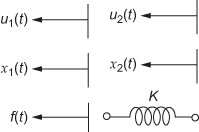
Fig. 1.18 ∣ Spring element with two displacements

![]()
![]()
Here, ![]() is measured in Newton (N) or Kg-m/s2.
is measured in Newton (N) or Kg-m/s2.
1.7.2 A Simple Translational Mechanical System
According to D'Alembert's principle, “The algebraic sum of the externally applied forces to any body is equal to the algebraic sum of the opposing forces restraining motion produced by the elements present in the body.”
A simple translational mechanical system with all the basic elements and its free body diagram are shown in Figs. 1.19 (a) and (b) respectively.

Fig. 1.19 ∣ (a) A simple translational mechanical system

Fig. 1.19 ∣ (b) Free body diagram
Let ![]() be the external force applied to the given system,
be the external force applied to the given system,
![]() be the opposing force produced by the element mass M,
be the opposing force produced by the element mass M,
![]() be the opposing force produced by the element damper B and
be the opposing force produced by the element damper B and
![]() be the opposing force produced by the element spring K.
be the opposing force produced by the element spring K.
Using D'Alembert's principle,
![]()
![]()
The above equation is referred to as D'Alembert's basic equation for translational mechanical systems.
Example 1.9: For the mechanical translational system shown in Fig. E1.9, obtain (i) differential equations and (ii) transfer function of the system.

Fig. E1.9
Solution: For the system given in Fig. E1.9, the input is ![]() and the outputs are
and the outputs are ![]() and
and ![]() .
.
Using D' Alembert's principle for the mass ![]() , we obtain
, we obtain
![]()
 (1)
(1)
For the mass ![]() , we obtain
, we obtain
![]()
 (2)
(2)
Taking Laplace transform of Eqn. (1) and Eqn. (2), we obtain
![]()
![]()
Representing the above equations in matrix form,

Using Cramer's rule, we obtain
![]()

![]()

![]()

![]()
![]()
Therefore, ![]()
![]()
and ![]()
![]()
Thus, the transfer function of the given mechanical system is given by


where ![]()
Example 1.10: For the mechanical translational system shown in Fig. E1.10, obtain (i) differential equations and (ii) transfer function of the system.

Fig. E1.10
Solution: For the system given in Fig. E1.10, the input is ![]() and the outputs are
and the outputs are ![]() and
and ![]() .
.
Using D' Alembert's principle for the mass ![]() ,
,
![]()

For the mass ![]() ,
, ![]()

Taking Laplace transform of the above equations, we obtain
![]()
![]()
Representing the above equations in matrix form,

Using Cramer's rule, we obtain
![]()

![]()

![]()

![]()
![]()
Therefore, ![]()
![]()
![]()
![]()
Thus, the transfer functions of the given mechanical system is given by


where ![]()
Example 1.11: For the mechanical translational system shown in Fig. E1.11, obtain (i) differential equations and (ii) transfer function of the system.

Fig. E1.11
Solution: For the system given in Fig. E1.11, the input is ![]() and the output is
and the output is ![]()
Using D' Alembert's principle for the mass ![]()
![]()
![]()
Taking Laplace transform on both the sides, we obtain
![]()
Hence, the transfer function of the system is given by

Example 1.12: For the mechanical translational system shown in Fig. E1.12, obtain (i) differential equations and (ii) transfer function of the system.

Fig. E1.12
Solution: For the system given in Fig. E1.12, the input is ![]() and the outputs are
and the outputs are ![]() and
and ![]() .
.
Using D' Alembert's principle for the mass ![]() ,
,
![]()
![]()
For the mass ![]() ,
, ![]()
![]()
Taking Laplace transform of the above equations, we obtain
![]()
![]()
Representing the above equations in matrix form,

Using Cramer's rule, we obtain
![]()

![]()

![]()

![]()
![]()
![]()
Therefore,
![]()

and ![]()
![]()
Thus, the transfer functions of the given mechanical system are given by

where ![]()
Example 1.13: For the mechanical translational system shown in Fig. E1.13, obtain (i) differential equations and (ii) transfer function of the system.

Fig. E1.13
Solution: For the system given in Fig. E1.13, the input is ![]() and the output is
and the output is ![]()
Using D' Alembert's principle for the mass ![]() ,
,
![]()
![]() (1)
(1)
Taking Laplace transform on both the sides, we obtain
![]()
Hence, the transfer function of the system is given by

Example 1.14: For the mechanical translational system shown in Fig. E1.14, obtain (i) differential equations and (ii) ![]()

Fig. E1.14
Solution: For the system shown in Fig. E1.14, the inputs are ![]() and
and ![]() and the outputs are
and the outputs are ![]() respectively.
respectively.
Using D' Alembert's principle for the mass ![]() ,
, ![]()

Using D' Alembert's principle for the mass ![]() ,
, ![]()

Taking Laplace transform on both the sides, we obtain
![]()
![]()
Representing the above equations in matrix form,

Using Cramer's rule, we obtain
![]()

![]()

![]()
Therefore,
![]()
![]()

Laplace transform of the given inputs f1(t) = 10 and f2(t) = 6 sin 5t are
![]()
![]()
Substituting the known values in the above equation, we obtain

![]()
Example 1.15: For the mechanical translational system shown in Fig. E1.15, obtain (i) differential equations and (ii) transfer function of the system.

Fig. E1.15
Solution: For the system given in Fig. E1.15, the input is ![]() and the outputs are
and the outputs are ![]() and
and ![]() .
.
Using D' Alembert's principle for the mass ![]() ,
, ![]()
 (1)
(1)
For the mass ![]() ,
, ![]()
 (2)
(2)
Taking Laplace transform of Eqn. (1) and Eqn. (2), we obtain
![]()
![]()
Representing the above equations in matrix form,

Using Cramer's rule, we obtain
![]()

![]()

![]()

![]()
Therefore,
![]()
![]()
![]()

Thus, the transfer functions of given mechanical system are given by


where ![]()
1.7.3 Rotational Mechanical System
The modeling of a linear passive rotational mechanical system can be obtained by using three basic elements: inertia, rotational spring and rotational damper. The modeling of a rotational mechanical system is similar to that of a translational mechanical system except that the elements of the system undergo a rotational instead of a translation movement.
The opposing torques due to inertia, rotational spring and rotational damper act on a system when the system is subjected to a torque. Using D'Alembert's principle, for a linear passive rotational mechanical system, the sum of all the torques acting on a body is zero (i.e., the sum of applied torques is equal to the sum of the opposing torques on a body). Angular displacement, angular velocity and angular acceleration are the variables used to describe a linear passive rotational mechanical system.
In rotational mechanical systems, the energy storage elements are inertia and rotational spring and the energy dissipating element is the rotational viscous damper. The analogous for the energy storage elements in an electrical circuit are the inductors and the capacitors and the analogous of energy dissipating element in an electrical circuit is the resistor.
The analogous of linear passive translational and rotational mechanical system is given in Table. 1.4.
Table 1.4 ∣ Analogous of translational and rotational mechanical system

Inertia Torque ![]()
The element that stores the kinetic energy of a rotational mechanical system is inertia. Inertia is considered to be a conservative element as the energy can be stored and retrieved without any loss. The factors on which the inertial element depends are geometric composition about the rotational axis and its density.
When a torque ![]() is applied to an inertia element J, it experiences an angular acceleration and it is shown in Fig. 1.20.
is applied to an inertia element J, it experiences an angular acceleration and it is shown in Fig. 1.20.

Fig. 1.20 ∣ Inertia element
According to Newton's second law, the inertia torque is proportional to the angular acceleration.
![]()
![]()
![]()
where J is the moment of inertia (kg-m2/rad), α is the angular acceleration (rad/s2), ω(t) is the angular velocity (rad/s), θ(t) is the angular displacement (rad) and TJ (t) is measured in Newton-meter (N-m).
Damping Torque ![]()
The description discussed about the damper in the linear translational mechanical system holds good for the linear rotational mechanical system except for the fact that force is replaced by torque. A damper element is represented by a dashpot system.
When a torque ![]() is applied to a damping element B, it experiences an angular velocity and it is shown in Fig. 1.21.
is applied to a damping element B, it experiences an angular velocity and it is shown in Fig. 1.21.

Fig. 1.21 ∣ Damper element
The damping torque is proportional to the angular velocity. Therefore,
![]()
![]()
![]()
where B is viscous friction coefficient (N-s/m), ω(t) is the angular velocity (rad/s) and θ(t) is the angular displacement (rad).
Damper element with two angular displacements and a single applied torque is shown in Fig. 1.22.

Fig. 1.22 ∣ Damper element with two angular displacements
![]()

Here, ![]() is measured in Newton-meter.
is measured in Newton-meter.
Torsional/rotational Spring Torque ![]()
In general, an element that stores potential energy in a rotational mechanical system is known as torsional/rotational spring. The analogous component of torsional/rotational spring in an electrical circuit is the capacitor that is used to store voltages. The opposing force developed by the rotational spring is directly related to the stiffness of the torsional/rotational spring and its total angular displacement from its equilibrium position.
When a torque ![]() is applied to a spring element K, it experiences an angular displacement and it is shown in Fig. 1.23.
is applied to a spring element K, it experiences an angular displacement and it is shown in Fig. 1.23.

Fig. 1.23 ∣ Torsional spring element
According to Hooke's law, spring torque is proportional to the angular displacement.
![]()
![]()
![]()
where ![]() and
and ![]()
where K is the spring constant (N-m/rad), i.e., K = ![]()
![]() is the angular velocity (rad/s) and
is the angular velocity (rad/s) and ![]() is the angular displacement (rad).
is the angular displacement (rad).
A spring element with two angular displacements is shown in Fig. 1.24.

Fig. 1.24 ∣ Torsional spring element with two angular displacements
![]()
![]()
Similarly,
![]()
![]()
Here, ![]() is measured in Newton-meter.
is measured in Newton-meter.
1.7.4 A Simple Rotational Mechanical System
According to D'Alembert's principle, “The algebraic sum of the externally applied torques to any body is equal to the algebraic sum of opposing torques restraining motion produced by the elements present in the body.”
A simple rotational mechanical system with all the basic elements and its free body diagram is shown in Fig.1.25 and Fig.1.26 respectively.

Fig. 1.25 ∣ A simple rotational mechanical system

Fig. 1.26 ∣ Free body diagram
Let ![]() be the external torque applied to the given system,
be the external torque applied to the given system,
![]() be the opposing torque produced by the element mass J,
be the opposing torque produced by the element mass J,
![]() be the opposing torque produced by the element damper B and
be the opposing torque produced by the element damper B and
![]() be the opposing torque produced by the element spring K.
be the opposing torque produced by the element spring K.
Using D'Alembert's principle, ![]()

The free body diagram of the system denoting the applied and opposing torques is shown in Fig. 1.26.
Restraining torques are given below:
Inertia torque ![]()
Damping torque ![]()
Spring torque ![]()
Example 1.16: Set up the differential equations for the mechanical system as shown in Fig. E1.16(a). Also, obtain its transfer function ![]() .
.

Fig. E1.16(a)
Solution: The given mechanical system is modified indicating the various angular displacements as shown in Fig. E1.16(b).

Fig. E1.16(b)
![]() is between the angular displacements
is between the angular displacements ![]() and
and ![]() .
.
![]() is under the angular displacement
is under the angular displacement ![]() .
.
![]() is between the angular displacements
is between the angular displacements ![]() and
and ![]() .
.
![]() is between the angular displacements
is between the angular displacements ![]() and
and ![]() .
.
![]() and
and ![]() are under the angular displacement
are under the angular displacement ![]() .
.
![]() is between the angular displacements
is between the angular displacements ![]() and
and ![]() .
.
![]() ,
, ![]() and
and ![]() are under the angular displacement
are under the angular displacement ![]() .
.
The equivalent mechanical system is shown in Fig. E1.16(c).

Fig. E1.16(c)
Method 1–Using substitution method
The differential equations are


![]()
![]()
Taking Laplace transform of the above five equations, we obtain
![]() (1)
(1)
![]() (2)
(2)
![]() (3)
(3)
![]() (4)
(4)
![]() (5)
(5)
Using Eqn. (1), we obtain
 (6)
(6)
Using Eqn. (2) and Eqn. (6), we obtain

Rearranging, we obtain

Therefore, ![]() (7)
(7)
where ![]()
Using Eqs. (3), (6) and (7), we obtain

Therefore, ![]() (8)
(8)
where ![]()
Using Eqs. (4), (7) and (8), we obtain
![]()
Therefore, ![]() (9)
(9)
where ![]()
Using Eqs. (9) and (8) in Eqn. (5), we obtain
![]()
The required transfer function of the given system is

where ![]()
![]()
![]()
![]()
![]()


Method 2–Using Cramer's rule
Writing Eqs. (1) through (5) in matrix form, we obtain
AX = Y
where

![]()
![]()
Required transfer function of the system,

Using Cramer's rule, we obtain
![]()
where 


![]()
![]()

![]()
where 
![]()


Therefore, ![]()


Therefore, the transfer function of the given system is

Example 1.17: For the mechanical rotational system shown in Fig. E1.17(a), obtain (i) differential equations and (ii) transfer function of the system.

Fig. E1.17(a)
Solution: For the given system, the input and output are applied torque ![]() and angular displacements are
and angular displacements are ![]() respectively. Hence, the required transfer function are
respectively. Hence, the required transfer function are  .
.
The system has two nodes and they are masses with moment of inertia ![]() and
and ![]() . The differential equations governing the system are given by torque balance equations at these nodes.
. The differential equations governing the system are given by torque balance equations at these nodes.
Let the angular displacement of mass with moment of inertia ![]() be
be ![]() . The Laplace transform of
. The Laplace transform of ![]() is
is ![]() . The free body diagram of J1 is shown in Fig. E1.17(b). The opposing torques acting on
. The free body diagram of J1 is shown in Fig. E1.17(b). The opposing torques acting on ![]() are marked as
are marked as ![]() and
and ![]() .
.
![]()
![]()

Fig. E1.17(b)
Using Newton's second law, we have
![]()
![]()
Taking Laplace transform, we obtain
![]() (1)
(1)
The free body diagram of ![]() is shown in Fig. E1.17(c). The opposing torque acting on
is shown in Fig. E1.17(c). The opposing torque acting on ![]() are marked as
are marked as ![]() and
and ![]() .
.

Fig. E1.17(c)
According to D' Alembert's principle, we have
![]()
![]()
Taking Laplace transform, we obtain
![]()
![]() (2)
(2)
The Eqs. (1) and (2) can be written in matrix form as

Applying Cramer's rule, we obtain

![]()
![]()

![]()
and 
Then, 

Thus, the overall transfer function of the given mechanical system is


1.8 Introduction to Analogous System
Two equations of similar form are defined as analogous systems. The advantage of analogous system is that, if the response of one system is known, then the other system is also known without actually solving it.
Generally, mechanical systems are converted into analogous electrical system. There is a similarity between the equilibrium equations (integro-differential equations) of electrical systems and mechanical systems. Due to this, an electrical equivalent can be drawn to a mechanical system.
Example of Analogous Systems
A transformer is analogical to a gear. The transformer adjusts its “voltage-to-current” ratio (V/I) based on the load applied on the transformer that is similar to that of a gear mechanism, by which it adjusts the “torque-to-speed” ratio (T/ω) based on the load requirement.
1.8.1 Advantages of Electrical Analogous System
The following are the advantages of electrical analogous system:
- Standard symbols are available in electrical systems such as resistance, inductance, capacitance, etc.
- Standard and simple laws are available in electrical system that makes it easier for calculation.
Example: Kirchhoff's laws, Thévenin's theorem, etc.
- (iii) It is easy to analyze a system for different parameter values in an electrical system, because R, L and C cannot be varied and their response can be seen.
In an electrical system, the dual networks are analogous systems and both are in electrical form. The analogous parameters in dual network are listed in Table 1.5.
Table 1.5 ∣ Analogous parameters in dual network

Types of Analogies
The different types of analogies are discussed as shown in Fig. 1.27.

Fig. 1.27 ∣ Types of analogies
1.8.2 Force–Voltage Analogy
Consider a simple translational mechanical system as shown in Fig. 1.28.

Fig. 1.28 ∣ Translational mechanical system
Using D'Alembert's principle, we have
Sum of the applied forces = sum of the opposing forces
 (1.6)
(1.6)
Consider a series RLC circuit as shown in Fig. 1.29.

Fig. 1.29 ∣ Series RLC circuit
Using KVL, the integro-differential equations can be written as
 (1.7)
(1.7)
Rearranging Eqs. (1.6) and (1.7), we obtain


Since the force of mechanical system is made analogous to the voltage of electrical system, the above two equations are represented as analogous system. This analogy is known as force–voltage (or) F–V analogy. The analogous parameters in F–V system are given in Table 1.6.
Table 1.6 ∣ F–V analogous parameters

1.8.3 Force–Current Analogy
Consider a simple parallel RLC Circuit as shown in Fig. 1.30.

Fig. 1.30 ∣ Parallel RLC circuit
Using KCL, the integro-differential equations can be written as follows:

 (1.8)
(1.8)
The force equation for translational mechanical system is
 (1.9)
(1.9)
Rearranging Eqs. (1.8) and (1.9), we obtain
![]()
![]()
Since the force of mechanical system is made analogous to the current of electrical system, the above two equations are represented as analogous system. This analogy is known as force–current (or) F–I analogy. The analogous parameters in F–I system are given in Table 1.7.
Table 1.7 ∣ F–I analogous parameters

The analogous variables for translational mechanical system and an electrical system are listed in Table 1.8.
Table 1.8 ∣ Analogous of F–V and F–I to translational mechanical system

Flow chart for problems related to force–voltage and force–current analogy
A flow chart for solving problems related to force–voltage and force–current analogy is shown in Fig. 1.31.

Fig. 1.31 ∣ Flow chart for force-voltage and force-current analogy system
Free Body Diagram
If all the opposing forces and applied forces acting on mass are marked separately, then it is named as free body diagram.
Example 1.18: For the mechanical system shown in Fig. E1.18(a), obtain (i) differential equations, (ii) force–voltage electrical analogous circuit and (iii) force–current electrical analogous circuit.

Fig. E1.18(a)
Solution:
Free body diagram of mass M1:
The mass spring damper system and the free body diagram of mass ![]() indicating the opposing and applied forces acting on it are shown in Figs. E1.18(b) and (c) respectively.
indicating the opposing and applied forces acting on it are shown in Figs. E1.18(b) and (c) respectively.


Fig. E1.18(b) Fig. E1.18(c)
Using D'Alembert's principle, we have
![]()
 (1)
(1)
Free body diagram of mass ![]() :
:
The mass spring damper system and the free body diagram of mass ![]() indicating the opposing and applied forces acting on it are shown in Figs. E1.21(d) and (e) respectively.
indicating the opposing and applied forces acting on it are shown in Figs. E1.21(d) and (e) respectively.


Fig. E1.18(d) Fig. E1.18(e)
Using D'Alembert's principle, we have
![]()
 (2)
(2)
Replacing the displacements with velocity in the Eqs. (1) and (2) governing the mechanical translational system, we obtain
![]() (3)
(3)
![]() (4)
(4)
(a) F–V Electrical Analogy
The F–V analogous elements for the mechanical system are given below:
![]()
![]()
![]()
![]()
![]()
![]()
![]()
![]()
The F–V analogous equations for Eqs. (3) and (4) are:
 (5)
(5)
 (6)
(6)
The F–V analogous circuit shown in Fig. E1.18(f) is constructed using the above Eqs. (5) and (6). Since the system contains two masses, the electrical circuit is constructed with two loops.
F–V Circuit:

Fig. E1.18(f)
(b) F–I Electrical Analogy
The F–I analogous elements for the mechanical system are given below:
![]()
![]()
![]()
![]()
![]()
![]()
![]()
![]()
The F–I analogous equations for Eqs. (3) and (4) are:
 (7)
(7)
 (8)
(8)
The F–I analogous circuit shown in Fig. E1.18(g) is constructed using the above Eqs. (7) and (8). Since the system contains two masses, the electrical circuit is constructed with two nodes.
F–I Circuit:

Fig. E1.18(g)
Example 1.19: For the mechanical system shown in Fig. E1.19(a), obtain (i) differential equations, (ii) force–voltage electrical analogous circuit and (iii) force–current electrical analogous circuit.

Fig. E1.19(a)
Solution:
Free body diagram of mass M2:
The mass spring damper system and the free body diagram of mass ![]() indicating the opposing and applied forces acting on it are shown in Figs. E1.19(b) and (c) respectively.
indicating the opposing and applied forces acting on it are shown in Figs. E1.19(b) and (c) respectively.


Fig. E1.19(b) Fig. E1.19(c)
Using D'Alembert's principle, we obtain
![]()
 (1)
(1)
Free body diagram of mass M1:
The mass spring damper system and the free body diagram of mass ![]() indicating the opposing and applied forces acting on it are shown in Figs. E1.19(d) and (e) respectively.
indicating the opposing and applied forces acting on it are shown in Figs. E1.19(d) and (e) respectively.


Fig. E1.19(d) Fig. E1.19(e)
Using D'Alembert's principle, we have
![]()
 (2)
(2)
(a) F–V Electrical Analogy
The F–V electrical analogous elements for the mechanical system are given below:
![]()
![]()
![]()
![]()
![]()
![]()
![]()
![]()
![]()
![]()
The F–V electrical analogous equations for Eqs. (1) and (2) are:
 (3)
(3)
 `(4)
`(4)
The F–V analogous circuit shown in Fig. E1.19(f) is constructed using the above Eqs. (3) and (4). Since the system contains two masses, the electrical circuit is constructed with two loops.
F–V Circuit:
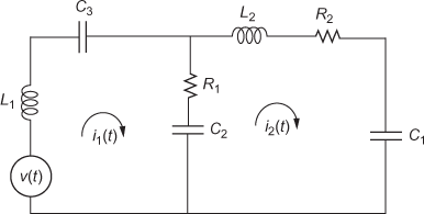
Fig. E1.19(f)
(b) F–I Electrical Analogy
The F–I electrical analogous elements for the mechanical system are given below:
![]()
![]()
![]()
![]()
![]()
![]()
![]()
![]()
![]()
![]()
The F–I electrical analogous equations for Eqs. (1) and (2) are:
 (5)
(5)
 (6)
(6)
The F–I analogous circuit shown in Fig. E1.19(g) is constructed using the Eqs. (5) and (6). Since the system contains two masses, the electrical circuit is constructed with two nodes.
F–I Circuit:
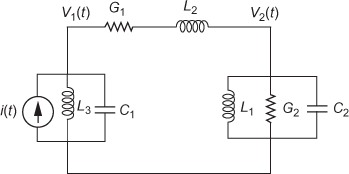
Fig. E1.19(g)
Example 1.20: For the mechanical translational system shown in Fig. E1.20(a), obtain (i) differential equations, (ii) F–V analogous circuit and (iii) F–I analogous circuit.
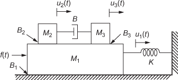
Fig. E1.20(a)
Solution:
Free body diagram of mass M3:
The mass spring damper system and the free body diagram of mass ![]() indicating the opposing and applied forces acting on it are shown in Figs. E1.20(b) and (c) respectively.
indicating the opposing and applied forces acting on it are shown in Figs. E1.20(b) and (c) respectively.

Fig. E1.20(b)

Fig. E1.20(c)
Using D'Alembert's principle, we have
![]()
 (1)
(1)
Free body diagram of mass M2:
The mass spring damper system and the free body diagram of mass ![]() indicating the opposing and applied forces acting on it are shown in Figs. E1.20(d) and (e) respectively.
indicating the opposing and applied forces acting on it are shown in Figs. E1.20(d) and (e) respectively.


Fig. E1.20(d) Fig. E1.20(e)
Using D'Alembert's principle, we have
![]()
![]() (2)
(2)
Free body diagram of mass M1:
The mass spring damper system and the free body diagram of mass ![]() indicating the opposing and applied forces acting on it are shown in Figs. E1.20(f) and (g) respectively.
indicating the opposing and applied forces acting on it are shown in Figs. E1.20(f) and (g) respectively.

Fig. E1.20(f)

ig. E1.20(g)
Using D'Alembert's principle, we have
![]()
![]() (3)
(3)
(a) F–V Electrical Analogy
The F–V analogous elements for the mechanical system are given by
![]()
![]()
![]()
![]()
![]()
![]()
![]()
![]()
![]()
![]()
![]()
![]()
The F–V analogous equations for Eqs. (1) through (3) are given by
![]() (4)
(4)
![]() (5)
(5)
![]() (6)
(6)
The F–V analogous circuit shown in Fig. E1.20(h) is constructed using the above Eqs. (4) through (6). Since the system contains three masses, the electrical circuit is constructed with three loops.
F–V Circuit:

Fig. E1.20(h)
(b) F–I Electrical Analogy
The F–I analogous elements for the mechanical system are given below:
![]()
![]()
![]()
![]()
![]()
![]()
![]()
![]()
![]()
![]()
![]()
The F–I analogous equations for Eqs. (1) through (3) are:
![]() (7)
(7)
![]() (8)
(8)
![]() (9)
(9)
The F–I analogous circuit shown in Fig. E1.20(i) is constructed using the Eqs. (7) through (9). Since the system contains three masses, the electrical circuit is constructed with three nodes.
F–I Circuit:

Fig. E1.20(i)
Example 1.21: For the mechanical system shown in Fig. E1.21(a), obtain (i) differential equations, (ii) force–voltage electrical analogous circuit and (iii) force–current electrical analogous circuit.
Solution:

Fig. E1.21(a)
Free body diagram of mass ![]() :
:
The mass spring damper system and the free body diagram of mass ![]() indicating the opposing and applied forces acting on it are shown in Figs. E1.21(b) and (c) respectively.
indicating the opposing and applied forces acting on it are shown in Figs. E1.21(b) and (c) respectively.


Fig. E1.21(b) Fig. E1.21(c)
Using D'Alembert's principle, we obtain
![]()
![]() (1)
(1)
Free body diagram of mass ![]() :
:
The mass spring damper system and the free body diagram of mass ![]() indicating the opposing and applied forces acting on it are shown in Figs. E1.21(d) and (e) respectively.
indicating the opposing and applied forces acting on it are shown in Figs. E1.21(d) and (e) respectively.


Fig. E1.21(d) Fig. E1.21(e)
Using D'Alembert's principle, we obtain
![]()
![]() (2)
(2)
(a) F–V Electrical Analogy
The F–V electrical analogous elements for the mechanical system are given below:
![]()
![]()
![]()
![]()
![]()
![]()
![]()
![]()
The F–V electrical analogous equations for Eqs. (1) and (2) are:
![]() (3)
(3)
![]() (4)
(4)
The F–V analogous circuit shown in Fig. E1.21(f) is constructed using the above Eqs. (3) and (4). Since the system contains two masses, the electrical circuit is constructed with two loops.
F–V Circuit:

Fig. E1.21(f)
(b) F–I Electrical Analogy
The F–I electrical analogous elements for the mechanical system are given below:
![]()
![]()
![]()
![]()
![]()
![]()
![]()
The F–I electrical analogous equations for Eqs. (1) and (2) are:
![]() (5)
(5)
![]() (6)
(6)
The F–I analogous circuit shown in Fig. E1.21(g) is constructed using the above Eqs. (5) and (6). Since the system contains two masses, the electrical circuit is constructed with two nodes.
F–I Circuit:

Fig. E1.21(g)
Example 1.22: For the mechanical system shown in Fig. E1.22(a), obtain (i) differential equations, (ii) force–voltage electrical analogous circuit and (iii) force–current electrical analogous circuit.

Fig. E1.22(a)
Solution:
Free body diagram of mass ![]() :
:
The mass spring damper system and the free body diagram of mass ![]() indicating the opposing and applied forces acting on it are shown in Figs. E1.22(b) and (c) respectively.
indicating the opposing and applied forces acting on it are shown in Figs. E1.22(b) and (c) respectively.


Fig. E1.22(b) Fig. E1.22(c)
Using D'Alembert's principle, we have
![]()
![]() (1)
(1)
Free body diagram of mass ![]() :
:
The mass spring damper system and the free body diagram of mass ![]() indicating the opposing and applied forces acting on it are shown in Figs. E1.22(d) and (e) respectively.
indicating the opposing and applied forces acting on it are shown in Figs. E1.22(d) and (e) respectively.


Fig. E1.22(d) Fig. E1.22(e)
Using D'Alembert's principle, we obtain
![]()
![]() (2)
(2)
Free body diagram of mass ![]() :
:
The mass spring damper system and the free body diagram of mass ![]() indicating the opposing and applied forces acting on it are shown in Figs. E1.22(f) and (g) respectively.
indicating the opposing and applied forces acting on it are shown in Figs. E1.22(f) and (g) respectively.


Fig. E1.22(f) Fig. E1.22(g)
Using D'Alembert's principle, we have
![]()
![]() (3)
(3)
(a) F–V Electrical Analogy
The F–V analogous elements for the mechanical system are given below:
![]()
![]()
![]()
![]()
![]()
![]()
![]()
![]()
![]()
![]()
![]()
![]()
The F–V analogous equations for Eqs. (1) through (3) are:
 (4)
(4)
 (5)
(5)
![]() (6)
(6)
The F–V analogous circuit shown in Fig. E1.22(h) is constructed using the above Eqs. (4) through Eqn. (6). Since the system contains three masses, the electrical circuit is constructed with three loops.
F–V Circuit:

Fig. E1.22(h)
(b) F–I Electrical Analogy
The F–I analogous elements for the mechanical system are given below:
![]()
![]()
![]()
![]()
![]()
![]()
![]()
![]()
![]()
![]()
![]()
The F–I analogous equations for Eqs. (1) through (3) are:
 (7)
(7)
 (8)
(8)
![]() (9)
(9)
The F–I analogous circuit shown in Fig. E1.22(i) is constructed using the above Eqs. (7) through (9). Since the system contains three masses, the electrical circuit is constructed with three nodes.
F–I Circuit:

Fig. E1.22(i)
1.8.4 Torque–Voltage Analogy
Consider a simple rotational mechanical system as shown in Fig.1.32.

Fig. 1.32 ∣ Rotational mechanical system
Using D'Alembert's principle, we have
Sum of the applied torques = sum of the opposing torques
![]() (1.10)
(1.10)
Consider a series RLC circuit as shown in Fig. 1.33.
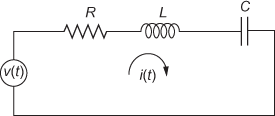
Fig. 1.33 ∣ Series RLC circuit
Applying KVL, we obtain
![]() (1.11)
(1.11)
Since the torque of the mechanical system is made analogous to the voltage of the electrical system, Eqs. (1.10) and (1.11) are represented as analogous system. This analogy is known as torque–voltage (or) T–V analogy. The analogous parameters in T–V system are given in Table 1.9.
Table 1.9 ∣ T–V analogous parameters

1.8.5 Torque–Current Analogy
Consider a simple rotational mechanical system as shown in Fig. 1.34.

Fig. 1.34 ∣ Rotational mechanical system
Using D'Alembert's principle, we have
![]() (1.12)
(1.12)
Consider parallel RLC Circuit as shown in Fig. 1.35.

Fig. 1.35 ∣ Parallel RLC circuit
Applying KCL, we obtain
![]()
![]() (1.13)
(1.13)
Since the torque of the mechanical system is made analogous to the current of the electrical system, Eqs. (1.12) and (1.13) are represented as analogous system. This analogy is known as torque–current (or) T–I analogy. The analogous parameters in T–I system are given in Table 1.10.
Table 1.10 ∣ T–I analogous parameters

The analogous variables for rotational mechanical system and electrical system are listed in Table 1.11.
Table 1.11 ∣ Analogous of T–V and T–I to rotational mechanical system

A flow chart for solving problems related to torque–voltage and torque–current analogy is shown in Fig. 1.36.

Fig. 1.36 ∣ Flow chart for torque-voltage and torque-current analogy system
Example 1.23: For the mechanical rotational system shown in Fig. E1.23(a), obtain (i) differential equations, (ii) T–V analogous circuit and (iii) T–I analogous circuit.

Fig. E1.23(a)
Solution: The given mechanical rotational system has three nodes, i.e., three moment of inertia of masses. The differential equations governing the mechanical rotational systems are given by torque balance equations at these nodes. Let the angular displacements of ![]() ,
, ![]() and
and ![]() be
be ![]() ,
, ![]() and
and ![]() respectively. The corresponding angular velocities are ω1(t), ω2(t) and ω3(t), respectively.
respectively. The corresponding angular velocities are ω1(t), ω2(t) and ω3(t), respectively.
Free body diagram for inertia J1:
The rotational mechanical system and the free body diagram of ![]() indicating the opposing and applied torques acting on it are shown in Figs. E1.23(b) and (c) respectively.
indicating the opposing and applied torques acting on it are shown in Figs. E1.23(b) and (c) respectively.


Fig. E1.23(b) Fig. E1.23(c)
Using D'Alembert's principle, we have
![]()
 (1)
(1)
Free body diagram for inertia J2:
The rotational mechanical system and the free body diagram of ![]() indicating the opposing and applied torques acting on it are shown in Figs. E1.23(d) and (e) respectively.
indicating the opposing and applied torques acting on it are shown in Figs. E1.23(d) and (e) respectively.


Fig. E1.23(d) Fig. E1.23(e)
Using D'Alembert's principle, we have
![]()
 (2)
(2)
Free body diagram for inertia J3:
The rotational mechanical system and the free body diagram of ![]() indicating the opposing and applied torques acting on it are shown in Figs. E1.23(f) and (g) respectively.
indicating the opposing and applied torques acting on it are shown in Figs. E1.23(f) and (g) respectively.

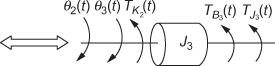
Fig. E1.23(f) Fig. E1.23(g)
Using D'Alembert's principle, we have
![]()
 (3)
(3)
Replacing the angular displacements by angular velocity in the differential Eqs. (1) through (3) governing the mechanical rotational system, we obtain
![]() (4)
(4)
![]() (5)
(5)
![]() (6)
(6)
T–V Electrical Analogy
The T–V analogous elements for the mechanical system are given below:
![]()
![]()
![]()
![]()
![]()
![]()
![]()
![]()
![]()
![]()
![]()
![]()
The T–V analogous equations of Eqs. (4) through (6) are:
 (7)
(7)
 (8)
(8)
 (9)
(9)
The T–V analogous circuit shown in Fig. E1.23(h) is constructed using the Eqs. (7) through (9). Since the system contains three inertial elements, the electrical circuit is constructed with three loops.
T–V Circuit:
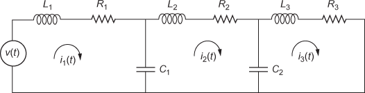
Fig. E1.23(h)
T–I Electrical Analogy
The T–I analogous elements for the mechanical system are given below:
![]()
![]()
![]()
![]()
![]()
![]()
![]()
![]()
![]()
![]()
![]()
![]()
The T–I analogous equations for Eqs. (4) through (6) are:
 (10)
(10)
 (11)
(11)
 (12)
(12)
The T–I analogous circuit shown in Fig. E1.23(i) is constructed using the Eqs. (10) through (12). Since the system contains three inertial elements, the electrical circuit is constructed with three nodes.
T–I Circuit:

Fig. E1.23(i)
Review Questions
- What do you mean by a system? Give examples.
- What do you mean by a control system? Give examples.
- What are the different types of control system?
- With the help of block diagram, write a note on open-loop systems.
- With the help of block diagram, write a note on closed-loop systems.
- Give a practical example for an open-loop system and explain it.
- Give a practical example for a closed-loop system and explain it.
- With the block diagram, illustrate the control of a car by the driver and identify the components of this closed-loop system.
- Distinguish the open-loop and closed-loop control systems.
- Explain the concept of principle of homogeneity and superposition.
- How are the systems classified based on principle of homogeneity and superposition?
- Define linear and non-linear systems with examples.
- How are the systems classified based on varying quantity and time?
- Define time-variant and time-invariant systems with examples.
- Define transfer function of a system.
- What are the features and advantages of transfer function?
- What are the disadvantages of transfer function?
- Determine the transfer function of the open-loop system.
- State whether transfer function is applicable to non-linear system.
- What are the types of closed-loop system?
- Why is negative feedback preferred in control system?
- Discuss the concept of negative feedback closed-loop system and derive its transfer function.
- Discuss the concept of positive feedback closed-loop system and derive its transfer function.
- What are the features or advantages of negative feedback control system?
- What is an error detector?
- What do you mean by modeling of systems?
- Explain with a neat flowchart, how to determine the transfer function of any physical systems.
- What are the basic elements used for modeling electrical system?
- What are the basic laws that are used for modeling electrical systems?
- Explain the relationship between current and voltage across different elements present in the electrical systems.
- How are the mechanical systems classified based on the movement of elements?
- What are the basic laws used for modeling mechanical systems?
- What do you mean by free body diagram of a mechanical system?
- What are the basic elements used for modeling translational mechanical system?
- Explain the mass element in translational mechanical system.
- Explain the damper element in translational mechanical system.
- What are the different types of friction in translational mechanical system? Discuss.
- Explain the spring element in the translational mechanical system.
- Write a short note on simple translational mechanical system.
- What are the basic elements used for modeling rotational mechanical system?
- Explain the inertia element in rotational mechanical system.
- Explain the damper element in rotational mechanical system.
- Explain the spring element in rotational mechanical system.
- Write a short note on simple rotational mechanical system.
- What do you mean by analogous system? Give examples.
- Explain the analogous of rotational and translational mechanical system.
- Explain the analogous existing within the electrical system.
- What are the advantages of electrical analogous system?
- What are the different types of analogies existing between the electrical and mechanical system?
- Explain the force–voltage analogy.
- Explain the force–current analogy.
- Tabulate the analogous parameters of the F–V analogy.
- Tabulate the analogous parameters of the F–I analogy.
- Explain with a neat flowchart, the procedure for determining the F–V and F–I analogous circuits.
- Explain the torque–voltage analogy.
- Explain the torque–current analogy.
- Tabulate the analogous parameters of the T–V analogy.
- Tabulate the analogous parameters of the T–I analogy.
- Explain with a neat flowchart, the procedure for determining the T–V and T–I analogous circuits.
- For the mechanical rotational system shown in Fig. Q1.60, obtain (i) differential equations, (ii) T–V analogous circuit and (iii) T–I analogous circuit.

Fig. Q1.60
- For the mechanical rotational system shown in Fig. Q1.61, obtain (i) differential equations, (ii) T–V analogous circuit and (iii) T–I analogous circuit.

Fig. Q1.61
- For the mechanical system shown in Fig. Q1.62, obtain (i) differential equations, (ii) transfer function of the system, (iii) force–voltage electrical analogous circuit and (iv) force–current electrical analogous circuit.

Fig. Q1.62
- For the mechanical system shown in Fig. Q1.63, obtain (i) differential equations, (ii) force–voltage electrical analogous circuit and (iii) force–current electrical analogous circuit.

Fig. Q1.63
- For the mechanical system shown in Fig. Q1.64, obtain (i) differential equations, (ii) force–voltage electrical analogous circuit and (iii) force-current electrical analogous circuit.
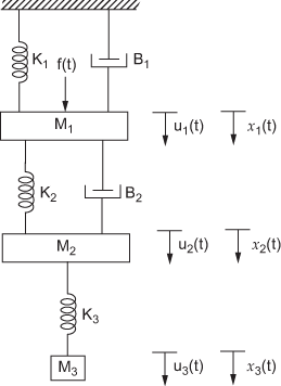
Fig. Q1.64
- For the mechanical system shown in Fig. Q1.65, obtain (i) differential equations, (ii) force–voltage electrical analogous circuit and (iii) force–current electrical analogous circuit.

Fig. Q1.65
- For the mechanical system shown in Fig. Q1.66, obtain (i) differential equations, (ii) force–voltage electrical analogous circuit and (iii) force–current electrical analogous circuit.

Fig. Q1.66
- For the mechanical system shown in Fig. Q1.67, obtain (i) differential equations, (ii) force–voltage electrical analogous circuit and (iii) force–current electrical analogous circuit.

Fig. Q1.67
- For the mechanical system shown in Fig. Q1.68, obtain (i) differential equations, (ii) force–voltage electrical analogous circuit and (iii) force–current electrical analogous circuit.

Fig. Q1.68
- For the mechanical system shown in Fig. Q1.69, obtain (i) differential equations, (ii) force–voltage electrical analogous circuit and (iii) force–current electrical analogous circuit.

Fig. Q1.69
- For the mechanical system shown in Fig. Q1.70, obtain (i) differential equations, (ii) force–voltage electrical analogous circuit and (iii) force–current electrical analogous circuit.

Fig. Q1.70
- For the mechanical system shown in Fig. Q1.71, obtain (i) differential equations, (ii) force–voltage electrical analogous circuit and (iii) force–current electrical analogous circuit.

Fig. Q1.71
- For the mechanical system shown in Fig. Q1.72, obtain (i) differential equations, (ii) force–voltage electrical analogous circuit and (iii) force–current electrical analogous circuit.

Fig. Q1.72
- For the mechanical system shown in Fig. Q1.73, obtain (i) differential equations, (ii) force–voltage electrical analogous circuit and (iii) force–current electrical analogous circuit.
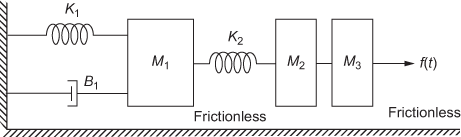
Fig. Q1.73
- For the mechanical system shown in Fig. Q1.74, obtain (i) differential equations and (ii) F–V electrical analogous circuit.

Fig. Q1.74
- For the mechanical system shown in Fig. Q1.75, obtain (i) differential equations, (ii) F–V electrical analogous circuit and (iii) F–I electrical analogous circuit.

Fig. Q1.75
- For the mechanical rotational system shown in Fig. Q1.76, obtain (i) differential equations and (ii) transfer function of the system.

Fig. Q1.76
- For the mechanical rotational system shown in Fig. Q1.77, obtain (i) differential equations and (ii) transfer function
 .
.
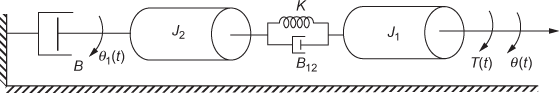
Fig. Q1.77
- For the mechanical translational system shown in Fig. Q1.78, obtain (i) differential equations and (ii) transfer function of the system.

Fig. Q1.78
- For the mechanical translation system shown in Fig. Q1.79, obtain (i) differential equations and (ii) transfer function of the system.

Fig. Q1.79
- For the mechanical translational system shown in Fig. Q1.80, obtain (i) differential equations and (ii) transfer function
 of the system.
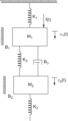
Fig. Q1.80
- Determine the transfer functions of the electrical networks shown in Fig. Q1.81.


-

Fig. Q1.81
- Write the integro-differential equations for the electrical network given in Fig. Q1.82.

Fig. Q1.82
- Determine the transfer function for a positive feedback system with a forward gain of 3 and a feedback gain of 0.2.
- For the mechanical translational system shown in Fig. Q1.84, obtain (i) differential equations and (ii) transfer function of the system.

Fig. Q1.84
- For the mechanical rotational system shown in Fig. Q1.85, obtain transfer function of the system.

Fig. Q1.85
- A negative feedback system is subjected to an input of 5 V. Determine the output voltage for the unity feedback system for the given values of forward gain: (i)
 = 1, (ii) = 5, (iii) = 50 and (iv) = 500
 - By simplifying the block diagram given in Fig. Q1.87, determine the value of the output
 .
.

Fig. Q1.87
- For the mechanical translational system shown in Fig. Q1.88, obtain (i) differential equations and (ii) transfer function of the system.

Fig. Q1.88
- For the mechanical system shown in Fig. Q1.89, obtain (i) differential equations, (ii) force–voltage electrical analogous circuit and (iii) force–current electrical analogous circuit.

Fig. Q1.89