4

SIGNAL FLOW GRAPH

4.1 Introduction

The diagrammatic or pictorial representation of a set of simultaneous linear algebraic ­equations of a more complicated system is known as signal flow graph (SFG). It shows the flow of signals in the system. It is important to note that the flow of signals in SFG is only in one direction. To represent the set of algebraic equations using SFG, it is necessary that those algebraic equations are to be represented in the s-domain. The transfer function of the system which is represented by SFG can be obtained by using Mason's gain formula.

The dependent and independent variables in the set of algebraic equations are ­represented by the nodes in the SFG. The branches are used to connect different nodes present in SFG. The connection between the different nodes is based on the relationship given in the ­algebraic equation. The arrow and the multiplication factor indicated on the branch of SFG represent the signal direction.

The SFG and the block diagram representation of a system yield the same transfer ­function; but when a system is represented by SFG, the transfer function is obtained easily and quickly without using the SFG reduction techniques.

4.1.1 Signal Flow Graph Terminologies

The terminologies used in SFG are explained with the help of SFG of a system as shown in Fig. 4.1.

Fig. 4.1 ∣ Signal flow graph of a system

Node

The variables present in the set of algebraic equations are represented by a point called node. The classification of nodes is shown in Fig. 4.2.

Fig. 4.2 ∣ Classification of nodes

The different types of nodes shown in Fig. 4.2 are explained in detail as follows:

Dummy node – (Special case)

If there is no source or sink node in the SFG of a system, then the input and output nodes can be created by adding branches with gain 1, which are known as dummy nodes. A schematic diagram representing the dummy node is shown in Fig. 4.3.

Fig. 4.3 ∣ A schematic diagram representing dummy node

Branch

The line segment joining the two nodes with a specific direction is known as a branch. The specific direction is indicated by an arrow in the branch. A schematic diagram representing the branch is shown in Fig. 4.4.

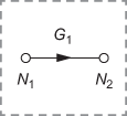
Fig. 4.4 ∣ A schematic diagram representing a branch

Source Node or Input Node

The type of node that has only outgoing branches is known as a source node or input node. It is the only independent variable present in the system as it does not depend on any other variables. All the other nodes present in the given system are dependent variables. The dotted line shown in Fig. 4.5 highlights the source node or the input node.

Fig. 4.5 ∣ Source node or Input node

Sink Node or Output Node

Sink node or output node is the one that has only incoming branches. The dotted lines shown in Fig. 4.6 highlight the sink node or output node.

Fig. 4.6 ∣ Sink node or output node

Mixed Node or Chain Node

Mixed or chain node is the one that has both incoming and outgoing branches. The dotted lines shown in Fig. 4.7 highlight the mixed node or chain node.

Fig. 4.7 ∣ Mixed node or chain node

Transmittance

When the signal flows from one node to another, the signal acquires a multiplication factor or gain. This gain between the two nodes is known as transmittance and it is indicated above the arrow mark in the branch. The transmittance between a dummy node and any other node is 1. The dotted lines shown in Fig. 4.8 highlight the transmittance between nodes and .

Fig. 4.8 ∣ Transmittance

Path

When the branches between the nodes are connected continuously in a specific direction and indicated by arrows on the branch, it is known as a path. The classification of a path is shown in Fig. 4.9.

Fig. 4.9 ∣ Classification of a path

Open Path

If the path starts from one node and ends at another node with none of the nodes traversed more than once is known as an open path.

Forward Path

In the open path, if the path starts from source or input node and ends at sink or output node with none of the nodes traversed more than once is known as forward path. The path represented by the dotted lines in Fig. 4.10 highlights one of the forward paths present in the SFG of the system shown in Fig. 4.1 in which the input node is and the output node is .

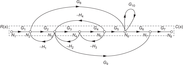
Fig. 4.10 ∣ Forward path

The other types of forward paths are shown in Figs. 4.11 and 4.12.

Fig. 4.11 ∣ Forward path

Fig. 4.12 ∣ Forward path

Closed Path or Loop or Feedback Path

If the path starts from one node and ends at the same node while traversing the other nodes for only one time, then it is known as a closed path or loop or a feedback path. The paths that are encircled by dotted lines in the schematic diagrams of Figs. 4.13 through 4.15 highlight the closed path or loop or feedback path for the SFG of the system shown in Fig. 4.1.

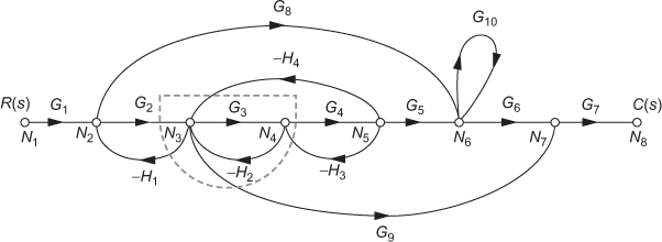
Fig. 4.13 ∣ Closed path or loop or feedback path

Fig. 4.14 ∣ Closed path or loop or feedback path

Fig. 4.15 ∣ Closed path or loop or feedback path

Self-Loop

The path that starts from one node and ends at the same node without traversing any other nodes is known as self-loop. The self-loop is also a type of closed path, since the path starts and ends at the same node. The loop encircled by the dotted lines in Fig. 4.16 highlights the self-loop.

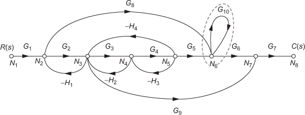
Fig. 4.16 ∣ Self-loop

Non-Touching Loops

If two or more individual loops existing in the given system do not have any common nodes between them, then the loops are known as non-touching loops. The loops encircled by the dotted lines in Fig. 4.17 through Fig. 4.21 highlight the non-touching loops as there are no ­common nodes.

Fig. 4.17 ∣ Non-touching loops

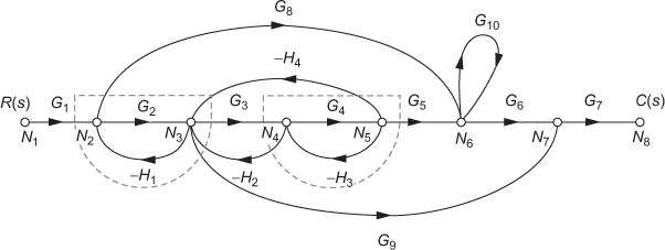
Fig. 4.18 ∣ Non-touching loops

Fig. 4.19 ∣ Non-touching loops

Fig. 4.20 ∣ Non-touching loops

Fig. 4.21 ∣ Non-touching loops

Gain

In a path, the transmittance existing in each of the branch can be multiplied to form a total transmittance of the path. This total transmittance is known as the gain of the path. The gains are classified as shown in Fig. 4.22 depending on the path.

Fig. 4.22 ∣ Classification of gain

Forward-Path Gain

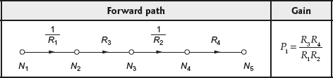
If the transmittance of the branch existing in the forward path is multiplied, then the resultant gain is known as forward-path gain. The forward-path gains for different forward paths existing in the SFG of the system are given in Table 4.1.

Table 4.1 ∣ Forward-path gains

Loop Gain or Feedback Path Gain

If the transmittance of the branch existing in the loop is multiplied, the resultant gain is known as loop or feedback path gain. The loop or feedback path gains for different loops existing in the SFG of the system shown in Fig. 4.1 are given in Table 4.2.

Table 4.2 ∣ Loop or feedback path gains

4.1.2 Properties of SFG

The important properties of SFG are:

1. There must be a cause-and-effect relationship between the algebraic equations for which the SFG has to be constructed.
2. SFG is applicable to linear time invariant systems.
3. Flow of signal in the SFG of the system is indicated by the arrow present in the branch between the nodes.
4. SFG for a particular system is not unique since the differential equations of a particular system can be written in different ways.
5. Variable or a signal given in the differential equation is indicated by a node.
6. Functional dependence of a node on another node is indicated by a branch.

4.1.3 SFG Algebra

The transfer function of the system represented using SFG can be obtained by applying certain algebraic rules to the SFG of the system. The following rules are used in Mason's gain formula for determining the transfer function of the given system.

Rule 1: Signal at a node: The signal at a node is obtained by multiplying the transmittance of the branch connecting the nodes and the signal at the previous node. The ­schematic diagram explaining the above concept is shown in Figs. 4.23(a) and 4.23(b).

Fig. 4.23 ∣ Signal at a node

Rule 2: When branches are in cascade connection: If the branches are pointing towards the same direction, then the branches are said to be in cascade connection as shown in Fig. 4.24(a). The transmittances indicated in each branch of the cascade connection can be multiplied to form a single branch as shown in Fig. 4.24(b).

Fig. 4.24 ∣ Branches in cascade connection

Rule 3: When branches are in parallel connection: If one or more branches pointing in the same direction originate and ends at the same node, then the branches in the SFG of the system are said to be in parallel connection as shown in Fig. 4.25(a). The ­transmittances indicated in each branch of the parallel connection can be added to form a single branch as shown in Fig. 4.25(b).

Fig. 4.25 ∣ Branches in parallel connection

Rule 4: Elimination of loops: The loops existing in the SFG of the system as shown in Fig. 4.26(a) can be eliminated as shown in Fig. 4.26(b). But while determining the transfer function of the system, this rule is not used.

Fig. 4.26 ∣ Elimination of loops

Rule 5: Elimination of mixed node: Mixed node with one or more incoming branches and an outgoing branch as shown in Fig. 4.27(a) can be eliminated by multiplying the transmittance of outgoing branch with transmittance of each of the incoming branches. The SFG of the system after eliminating such mixed node is shown in Fig. 4.27(b).

Fig. 4.27 ∣ Elimination of mixed node

4.1.4 Mason's Gain Formula for SFG

The transfer function or overall gain of the system represented by SFG can be obtained using Mason's gain formula given by

where is the forward-path gain, n is the total number of forward paths and

Here is the sum of all individual loop gains, is the sum of the product of gains of all possible combination of two non-touching loops and is the sum of the product of gains of all possible combination of three non-touching loops. Therefore,

Δ_k = 1 − (sum of individual loop gains that do not touch the k^th forward path)

4.1.5 Signal Flow Graph From Differential Equation

The flowchart to determine the signal flow graph from a set of differential equations is shown in Fig. 4.28.

Fig. 4.28 ∣ Flow chart to determine SFG from a set of differential equations.

Obtain (a) SFG for the given system and (b) transfer functions of the system using Mason's gain formula:

for and

Solution:

Given (1)

(2)

(a) To obtain SFG for the given system:

For the given equations, the inputs are and . In addition, the outputs for the given equations are and respectively.

Step 1:The SFG for Eqn. (1) is shown in Fig. E4.1(a).

Fig. E4.1(a)

Step 2:The SFG for Eqn. (2) is shown in Fig. E4.1(b).

Fig. E4.1(b)

Step 3:The SFG for the system represented by the Eqs. (1) and (2) can be obtained by combining the individual signal flow graphs that are shown in Figs. E4.1(a) and (b). The SFG for the system is shown in Fig. E4.1(c).

Fig. E4.1(c)

(b) To obtain the transfer function of the system:

1. (1) To determine

   To determine the required transfer function, it is necessary to make the input zero. Hence, the required transfer function will be

   

Step 1:The modified SFG from the original SFG with nodes marked is shown in Fig. E4.1(d).

Fig. E4.1(d)

Step 2:The number of forward paths n in the SFG shown in Fig. E4.1(d) is one and the gain corresponding to the forward path is given in Table E4.1(a).

Table E4.1(a) ∣ Gain for the forward path

Step 3:The number of individual loops m present in the SFG shown in Fig. E4.1(d) is and the gain corresponding to each loop is given in Table E4.1(b).

Table E4.1(b) ∣ Individual loop gains

Step 4:Then the individual loop gains are added together to determine the total individual loop gain . Therefore,

, where

Step 5:Determine the number of possible combination of loops , where , which has no node in common in the SFG. For the given combination of loop , determine the product of gains of all possible combination of non-touching loops , where For the given SFG, the product of gains of all possible combination of two non-touching loops is given in Table E4.1(c).

Table E4.1(c) ∣ Product of gains of combination of two non-touching loops

Step 6:Determine the sum of gain of loops , where , for each combination of non-touching loops . In the given problem, there exists only one different combination of two loops that have no node in common. Hence, , where is zero.

Therefore,

Step 7:Determine for the given SFG. Since there exists no part of the graph that does not touch the forward path in the given SFG, the value of is one.

Step 8:The transfer function of the system using Mason's gain formula is given by

(2) To determine

To determine the required transfer function, it is necessary to make the input zero. Hence, the required transfer function will be .

Step 1:The modified SFG from the original SFG with nodes marked is shown in Fig. E4.1(e).

Fig. E4.1(e)

Step 2:The number of forward paths n in the SFG shown in Fig. E4.1(d) is 1 and the gain corresponding to the forward path is given in Table E.4.1(d).

Table E4.1(d) ∣ Gain for the forward path

Step 3:The number of individual loops m present in the SFG shown in Fig. E4.1(d) is and the gain corresponding to each loop is given in Table E4.1(e).

Table E4.1(e) ∣ Individual loop gains

Step 4:Then, the individual loop gains are added together to determine the total individual loop gain . Therefore,

, where

Step 5:Determine the number of possible combination of loops , where,which has no node in common in the SFG. For the given combination of loop , determine the product of gains of all possible combination of non-touching loops , where For the given SFG, the product of gains of all possible combination of two non-touching loops is given in Table E4.1(f).

Table E4.1(f) ∣ Product of gains of combination of two non-touching loops

Step 6:Determine the sum of gain of loops , where , for each combination of non-touching loops . In the given problem, there exists only one different combination of two loops that have no node in common. Hence, , where is zero. Therefore, .

Step 7:Determine , where for the given SFG. The part of the graph that does not touch the forward path and its corresponding gain are given in Table E4.1(g).

Table E4.1(g) ∣ Determination of

Step 8:The transfer function of the system using Mason's gain formula is given by

Fig. E4.2(a)

Solution:

Step 1:The SFG shown in Fig. E4.2(a) can be modified as shown in Fig. E4.2(b) by using different variables at different nodes.

Fig. E4.2(b)

Step 2:To obtain the individual block diagram for the variables in the SFG, it is necessary to obtain its corresponding equations. For the SFG shown in Fig. E4.2(b), there are five variables of which is the input variable and others are output variables.

The equations for each variable present in the SFG are given below:

For variable , the equation is given by

(1)

For variable , the equation is given by

(2)

For variable , the equation is given by

(3)

For variable , the equation is given by

(4)

Step 3:Once the equation of each variable present in the SFG is obtained, the individual block diagram for each of the equation is drawn. Hence, the individual block diagrams for the Eqs. (1) to (4) are shown in Figs. E4.2(c) through (f).

Fig. E4.2(c)

Fig. E4.2(d)

Fig. E4.2(e)

Fig. E4.2(f)

Step 4:The individual block diagrams shown in Figs. E4.2(c) through (f) are combined in an appropriate way and the block diagram equivalent to the given SFG is shown in Fig. E4.2(g).

Fig. E4.2(g)

Fig. E4.3

Solution:

Step 1:For the given SFG, and its corresponding gain is given in Table E4.3(a).

Table E4.3(a) ∣ Gains for different forward paths

Step 2:For the given SFG, and its corresponding gain is given in Table E4.3(b).

Table E4.3(b) ∣ Individual loop gains

Step 3:Then, the gains of individual loops are added together to get the total individual loop gain . Therefore,

, where

Step 4:For the given SFG, the product of gains of all possible combination of two and three non-touching loops is given in Tables E4.3(c) and (d) respectively.

Table E4.3(c) ∣ Product of gains of combination of two non-touching loops

Table E4.3(d) ∣ Product of gains of combination of three non-touching loops

Step 5:In the given problem, there only exists a combination of two and three loops that have no node in common. Hence, , where is zero.

Therefore,

and

Step 6:Since there exists no part of the graph that does not touch the forward paths in the given SFG, the values of and are 1.

Step 7:The transfer function of the system using Mason's gain formula is given by

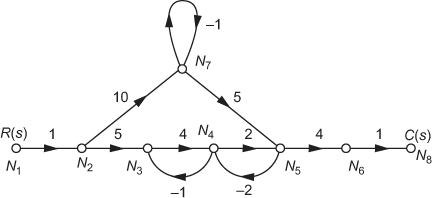
Fig. E4.4

Solution:

Step 1:The number of forward paths n in the SFG shown in Fig. E4.4 is and the corresponding gain of the forward path is given in Table E4.4(a).

Table E4.4(a) ∣ Gain for the forward path

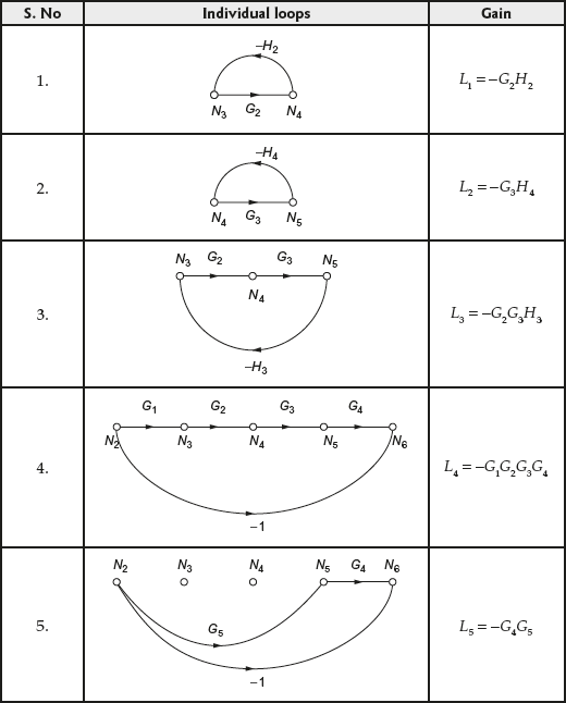
Step 2:The number of individual loops present in the SFG shown in Fig. E4.4 is and the corresponding gain of each loop is given in Table E4.4(b).

Table E4.4(b) ∣ Individual loop gains

Step 3:For the given SFG, .

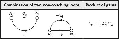
Step 4:For the given SFG, the product of gains of all possible combination of two non-touching loops is given in Table E4.4(c).

Table E4.4(c) ∣ Product of gains of combination of two non-touching loops

Step 5:In the given problem, there exist two different combination of two loops that have no node in common. Hence, and is zero.

Step 6:The part of the graph that does not touch the first and second forward paths, the ­corresponding gain and respective values are given in Tables E4.4(d) and (e) ­respectively.

Table E4.4(d) ∣ Determination of

Table E4.4(e) ∣ Determination of

Step 7:The transfer function of the system using Mason's gain formula is given by

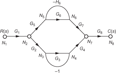
Fig. E4.5

Step 1: The number of forward paths in the SFG shown in Fig. E4.5 is and the gain corresponding to the forward path is given in Table E4.5(a).

Table E4.5(a) ∣ Gain for the forward path

Step 2:The number of individual loops present in the SFG shown in Fig. E4.5 is and the gain corresponding to each loop is given in Table E4.5(b).

Table E4.5(b) ∣ Individual loop gains

Step 3:For the given SFG,

Step 4:For the given SFG, the product of gains of all possible combination of two non-touching loops is given in Table E4.5(c).

Table E4.5(c) ∣ Product of gains of combination of two non-touching loops

Step 5:In the given problem, there exists only one different ­combination of two loops that have no node in common. Hence, , where is zero.

Therefore,

Step 6:The part of the graph that does not touch the first and second forward path, its corresponding gain and respective values are given in Tables E4.5(d) and (e).

Table E4.5(d) ∣ Determination of

Table E4.5(e) ∣ Determination of

Step 7:The transfer function of the system using Mason's gain formula is given by

.

Fig. E4.6

Solution:

Step 1:For the given SFG, and the corresponding gain is given in Table E4.6(a).

Table E4.6(a) ∣ Gains for different forward paths

Step 2:For the given SFG, and its corresponding gain is given in Table E4.6(b).

Table E4.6(b) ∣ Individual loop gains

Step 3:For the given SFG,

Step 4:For the given SFG, the product of gains of all possible combination of two non-touching loops is given in Table E4.6(c).

Table E4.6(c) ∣ Product of gains of combination of two non-touching loops

Step 5:In the given problem, there exists only one combination of two loops that have no node in common. Hence, , where is zero. Therefore,

Step 6:The part of the graph that does not touch the first and second forward path, its ­corresponding gain and respective values are given in Tables E4.6(d) and (e).

Table E4.6(d) ∣ Determination of

Table E4.6(e) ∣ Determination of

But there is no part of the graph that does not touch the other forward paths in the given SFG, the value of , where is one.

Step 7:The transfer function of the system using Mason's gain formula is given by

Fig. E4.7

Solution:

Step 1:The number of forward paths in the SFG shown in Fig. E4.7 is and the gain corresponding to the forward path is given in Table E4.7(a).

Table E4.7(a) ∣ Gain for the forward path

Step 2:The number of individual loops present in the SFG shown in Fig. E4.7 is and the gain corresponding to each loop is given in Table E4.7(b).

Table E4.7(b) ∣ Individual loop gains

Step 3:For the given SFG,

Step 4:For the given SFG, the product of gains of all possible combination of two non-touching loops is given in Table E4.7(c).

Table E4.7(c) ∣ Product of gains of combination of two non-touching loops

Step 5:In the given problem, there exist different combination of two loops which have no node in common. Hence, , where is zero. Therefore,

Step 6:Since there exist no part of the graph which does not touch the second forward path, the value of is 1. The part of the graph which does not touch the first forward path and its corresponding gain are given in Table E4.7(d).

Table E4.7(d) ∣ Determination of

Step 7:The transfer function of the system using Mason's gain formula is given by

Fig. E4.8(a)

Solution: To determine the transfer function of an electrical circuit, the following ­procedure has to be followed:

Step A: Determine the block diagram of the given electrical circuit.

Step B: Determine the SFG of the system equivalent to the block diagram.

Step C: Determine the transfer function of the system using Mason's gain formula.

Step A: To determine the block diagram of the given electrical circuit: Admittances Y₁ and Y₂ are in series path. Impedances Z₂ and Z₄ are in shunt path. The node voltages in the given electrical circuit are and . The loop currents in the given electrical circuit are and .

The current flowing through each element present in the series path is found by using node voltages.

1. The current flowing through admittance Y₁ is given by

   (1)

2. The current flowing through admittance Y₂ is given by

   (2)

The voltages across each element present in the shunt path are found out by using loop currents.

1. The voltage across Z₂ is given by

   (3)

2. The voltage across Z₄ is given by

   (4)

Individual block diagrams representing each of the above equations can be determined by examining the input and output of the respective equation. Then, the determined ­individual block diagrams can be combined in an appropriate way to represent the given electrical ­circuit.

To determine the individual block diagrams:

For Eqn. (1):

Taking Laplace transform of Eqn. (1), we obtain

(5)

where the inputs are , and the output is . Hence, the block diagram for the above equation is shown in Fig. E4.8(b).

Fig. E4.8(b)

For Eqn. (2):

Taking Laplace transform of Eqn. (2), we obtain

(6)

where the inputs are , and the output is . Hence, the block diagram for the above equation is shown in Fig. E4.8(c).

Fig. E4.8(c)

For Eqn. (3):

Taking Laplace transform of Eqn. (3), we obtain

(7)

where the inputs are and and the output is . Hence, and the block diagram for the above equation is shown in Fig. E4.8(d).

Fig. E4.8(d)

For Eqn. (4):

Taking Laplace transform of Eqn. (4), we obtain

(8)

where the input is and the output is . Hence, the block diagram for the above equation is shown in Fig. E4.8(e).

Fig. E4.8(e)

Hence, the overall block diagram for the given electrical circuit shown in Fig. E4.8(a) is obtained by interconnecting the block diagrams shown in Fig. E4.8(b) through (e). The overall block diagram of the given electrical circuit is shown in Fig. E4.8(f).

Fig. E4.8(f)

Step B: SFG for the given electrical circuit: The SFG equivalent of the block diagram shown in Fig. E4.8(f) is shown in Fig. E4.8(g).

Fig. E4.8(g)

Step C: To determine the transfer function of the given electrical circuit

Step 1: For the given SFG, and the gain corresponding to the forward path is given in Table E4.8(a).

Table E4.8(a) ∣ Gain corresponding to the forward path

Step 2:For the given SFG, and the corresponding loop gains are given in Table E4.8(b).

Table E4.8(b) ∣ Individual loop gains

Step 3:For the given SFG,

Step 4:For the given SFG, the product of gains of all possible combination of two non-touching loops is given in Table E4.8(c).

Table E4.8(c) ∣ Product of gains of combination of two non-touching loops

Step 5:In the given problem, there exists one combination of two loops that have no node in common. Hence, , where is zero. Therefore,

Step 6:Since there exists no part of the graph that does not touch the first forward path in the given SFG, the value of is 1.

Step 7:The transfer function of the system using Mason's gain formula is given by

Solution: As the given transfer function is difficult to factorize, we can use the third method (observer canonical form) to obtain SFG of the system. The steps to obtain SFG of the system from transfer function are given below:

Step 1:The transfer function of the system (both numerator and denominator) should be divided by the highest power present in the respective terms. Therefore,

(1)

Step 2:Cross-multiplying the Eqn. (1), we obtain

(2)

Step 3:Combining the terms of like powers of integration gives

(3)

Step 4:From Eqn. (3), the SFG of the system can be drawn. It is very clear that the system requires three integration ( highest power of ). Hence, as an initial step to draw the SFG of the system, a straight line with three integration is drawn as shown in Fig. E4.9(a).

Fig. E4.9(a)

Step 5:By integrating the first term of Eqn. (3), i.e., once, part of an output can be obtained. The integration of the first term is shown in Fig. E4.9(b).

Fig. E4.9(b)

Step 6:By integrating the second term of Eqn. (3), i.e., 3R(s) − 3C(s), another part of the output can be obtained. The integration of the second term is shown in Fig. E4.9(c). As the second term has to be integrated twice, it must be present in the existing loop, i.e., in Fig. E4.9(b).

Fig. E4.9(c)

Step 7:By integrating the third term of Eqn. (3), i.e., 3R(s) − 3C(s), the whole output can be obtained. The integration of the third term is shown in Fig. E4.9(d). As the second term has to be integrated twice, it must be present in the existing loop, i.e., in Fig. E4.9(c).

Fig. E4.9(d)

Hence, the diagram shown in Fig. E4.9(d) is the SFG representation of the given transfer function.

Fig. E4.10(a)

Solution:

Step 1:The SFG for the block diagram shown in Fig. E4.10(a) is shown in Fig. E4.10(b).

Fig. E4.10(b)

Step 2:For the given SFG, and the gains corresponding to each forward path are given in Table E4.10(a).

Table E4.10(a) ∣ Gains for different forward paths

Step 3:For the given SFG, and the corresponding loop gains are given in Table E4.10(b).

Table E4.10(b) ∣ Individual loop gains

Step 4:For the given SFG,

Step 5:For the given SFG,

Step 6:Determine , where for the given SFG. Since there exists no part of the graph that does not touch the first and second forward path in the given SFG, the values of and are 1.

Step 7:The transfer function of the system using Mason's gain formula is given by

(1)

Verification using block diagram reduction technique

Step 1:The SFG of a system is shown in Fig. E4.10(a). The equivalent block diagram of the system is shown in Fig. E4.10(c).

Fig. E4.10(c)

Step 2:The takeoff point that exists between the blocks and as shown in Fig. E4.10(d) is shifted before the block . The resultant block diagram is shown in Fig. E4.10(e).

Fig. E4.10(d)

Step 3:The blocks in series as shown in Fig. E4.10(e) can be combined to form a single block and the resultant block diagram is shown in Fig. E4.10(f).

Fig. E4.10(e)

Step 4:The blocks in parallel as shown in Fig. E4.10(f) can be combined to form a single block. In addition, the summing point existing after the block as shown in Fig. E4.10(f) is shifted before the block. The resultant block diagram is shown in Fig. E4.10(g).

Fig. E4.10(f)

Step 5:The blocks in series as shown in Fig. E4.10(g) can be combined to form a single block. In addition, the two summing points that exist before the block as shown in Fig. E4.10(g) can be interchanged. The resultant block diagram is shown in Fig. E4.10(h).

Fig. E4.10(g)

Step 6:The feedback path shown in Fig. E4.10(h) can be reduced to form a single block. The resultant block diagram is shown in Fig. E4.10(i).

Fig. E4.10(h)

Step 7:The blocks in series as shown in Fig. E4.10(i) can be reduced to form a single block. In addition, the common takeoff point as shown in Fig. E4.10(i) can be separated. The resultant block diagram is shown in Fig. E4.10(j).

Fig. E4.10(i)

Step 8:The feedback loop existing in the block diagram as shown in Fig. E4.10(j) can be reduced to form a single block and the resultant block diagram is shown in Fig. E4.10(k).

Fig. E4.10(j)

Step 9:The feedback loop existing in the block diagram as shown in Fig. E4.10(k) can be reduced to determine the transfer function of the system whose SFG is shown in Fig. E4.10(a).

Fig. E4.10(k)

Hence, the transfer function of the system is obtained as

(2)

From Eqs. (1) and (2), it is clear that the transfer function of the system shown in Fig. E4.10(a) using SFG and block diagram reduction techniques are the same.

Fig. E4.11(a)

Solution:

(a) To determine the transfer function by using block diagram reduction technique

Step 1:The blocks in parallel as shown in Fig. E4.11(b) are combined to form a single block. The resultant block diagram is shown in Fig. E4.11(c).

Fig. E4.11(b)

Step 2:The blocks in series as shown in Fig. E4.11(c) are combined to form a single block. The resultant block diagram is shown in Fig. E4.11(d).

Fig. E4.11(c)

Step 3:The summing point present after the block as shown in Fig. E4.11(d) can be moved after the block . The resultant block diagram is shown in Fig. E4.11(e).

Fig. E4.11(d)

Step 4:The blocks in series as shown in Fig. E4.11(e) are combined to form a single block. Also, the two summing points that exist in the block diagram shown in Fig. E4.11(e) can be combined to obtain a single summing point and the resultant block diagram is shown in Fig. E4.11(f).

Fig. E4.11(e)

Step 5:The summing point with three inputs as shown in Fig. E4.11(f) is split into two summing points and the resultant block diagram is shown in Fig. E4.11(g).

Fig. E4.11(f)

Step 6:The blocks in parallel and the feedback loop existing in the block diagram as shown in Fig. E4.11(g) can be reduced to form a single block and the resultant block diagram is shown in Fig. E4.11(h).

Fig. E4.11(g)

Step 7:The blocks in series as shown in Fig. E4.11(h) can be combined to determine the transfer function of the system.

Fig. E4.11(h)

Hence, the transfer function of the given system is obtained as

(1)

(b) To determine transfer function by using SFG

Step 1:The SFG for the given block diagram shown in Fig. E4.11(a) is drawn and is shown in Fig. E4.11(i).

Fig. E4.11(i)

Step 2: The number of forward paths in the SFG, shown in Fig. E4.11(i) is 4 and the gain corresponding to the forward path is given in Table E4.11(a)

Table E4.11(a) ∣ Gain for the forward path

Step 3:The number of individual loops present in the SFG shown in Fig. E4.11(a) is and the gain corresponding to each loop is given in Table E4.11(b).

Table E4.11(b) ∣ Individual loop gains

Step 4:For the given SFG,

Step 5:Since there exists no combination of two non-touching loops without a common node in the given SFG, the product of gains of the non-touching loops is zero, i.e., higher orders of are zero, where j = 2, 3, …, m.

Step 6:Since there exists no part of the graph that does not touch the forward paths in the given SFG, the values of are one.

Step 7:The transfer function of the system using Mason's gain formula is given

(2)

From Eqs. (1) and (2), it is clear that the transfer functions obtained for the system shown in Fig. E4.11(a) using block diagram reduction technique and SFG technique are same.

Fig. E4.12(a)

Solution:

Step 1:For the given SFG, and the gains corresponding to each forward path are given in Table E4.12(a).

Table E4.12(a) ∣ Gains for different forward paths

Step 2:For the given SFG, and the corresponding loop gains are given in Table E4.12(b).

Table E4.12(b) ∣ Individual loop gains

Step 3:For the given SFG,

Step 4:For the given SFG, the product of gains of all possible combination of two non-touching loops is given in Table E4.12(c).

Table E4.12(c) ∣ Product of gains of combination of two non-touching loops

Step 5:In the given problem, there exist only two different ­combination of two loops that have no node in common. Hence, S_j, where is zero. Therefore,

Step 6:Since there exists no part of the graph that does not touch the first forward path in the given SFG, the value of is 1.

But, the part of the graph that does not touch the second forward path and its corresponding gain are given in Table E4.12(d).

Table E4.12(d) ∣ Determination of

Step 7:The transfer function of the system using Mason's gain formula is

Fig. E4.13(a)

Solution:

Step 1:The SFG for the block diagram shown in Fig. E4.13(a) is shown in Fig. E4.13(b).

Fig. E4.13(b)

Step 2:The number of forward paths in the SFG, n shown in Fig. E4.13(b) is 1 and the gain corresponding to the forward path is given in Table E4.13(a).

Table E4.13(a) ∣ Gain for the forward path

Step 3:The number of individual loops present in the SFG shown in Fig. E4.13(b) is and the gain corresponding to each loop is given in Table E4.13(b).

Table E4.13(b) ∣ Individual loop gains

Step 4:For the given SFG,

Step 5:For the given SFG, the product of gains of all possible combination of two non-touching loops is given in Table E4.13(c).

Table E4.13(c) ∣ Product of gains of combination of two non-touching loops

Step 6:In the given problem, there exists one combination of two loops that have no node in common. Hence, S_j, where is zero. Therefore,

Step 7:Since there exists no part of the graph that does not touch the forward paths in the given SFG, the values of are 1.

Step 8:The transfer function of the system using Mason's gain formula is

Fig. E4.14(a)

Solution: To determine the transfer function of the system, the following steps have to be followed:

1. The transfer function of the system, is obtained by considering as the input and as the output.
2. Then, the transfer function of the system, is obtained by considering as the input and as the output.
3. Then, the required transfer function of the system, is obtained as

(a) To determine the transfer function of the system,

Step 1:The number of forward paths in the SFG, n shown in Fig. E4.14(a) is 2 and the gain corresponding to the forward path is given in Table E4.14(a).

Table E4.14(a) ∣ Gain for the forward path

Step 2:The number of individual loops present in the SFG shown in Fig. E4.14(a) is and the gain corresponding to each loop is given in Table E4. 14(b).

Table E4.14(b) ∣ Individual loop gains

Step 3:For the given SFG,

Step 4:For the given SFG, the product of gains of all possible combination of two non-touching loops is given in Table E4.14(c).

Table E4.14(c) ∣ Product of gains of combination of two non-touching loops

Step 5:In the given problem,

Step 6:The next step is to determine for the given SFG. Since there exists no part of the graph that does not touch the forward paths in the given SFG, the values of are one.

Step 7:The transfer function of the system using Mason's gain formula is given by

(b) To determine the transfer function of the system,

Step 1: The modified SFG for determining the transfer function of the system, is shown in Fig. E4.14(b).

Fig. E4.14(b)

Step 2:The number of forward paths in the SFG, n shown in Fig. E4.14(b) is 1 and the gain corresponding to the forward path is given in Table E4.14(d).

Step 3:The number of individual loops present in the SFG shown in Fig. E4.14(a) is and the gain corresponding to loop is given in Table E4.14(e).

Step 4:For the given SFG,

Step 5:Since there exists no combination of two non-touching loops without a common node in the given SFG, the product of gains of the non-touching loops is zero, i.e., higher orders of are zero, where j = 2, 3, …, m.

Step 6:The next step is to determine for the given SFG. Since there exists no part of the graph that does not touch the forward paths in the given SFG, the value of is 1.

Step 7:The transfer function of the system using Mason's gain formula is given by

(c) To determine the required transfer function of the system,

Required transfer function,

Fig. E4.15(a)

Solution: To determine the transfer function of an electrical circuit, the following procedure has to be followed:

Step A: Determine the individual SFG of the electrical equations.

Step B: Determine the SFG for the given electrical circuit.

Step C: Determine the transfer function of the given electrical circuit using Mason's gain formula.

Step A: To determine the individual SFG of the electrical equations.

The currents flowing through R₁ is i₁(t) and R₂ is i₂(t). Hence, using node voltages v₂(t) and v₃(t), the currents i₁(t) and i₂(t) are obtained as

(1)

(2)

Also, from Fig. E4.15(a), we obtain

(3)

Equating Eqs. (2) and (3) and simplifying, we obtain

(4)

The voltage across R₃ is given by

(5)

The voltage across R₄ is given by

(6)

For Eqn. (1):

Taking Laplace transform of Eqn. (1), we obtain

(7)

where the input is and and the output is . Hence, the SFG of the above equation is shown in Fig. E4.15(b).

Fig. E4.15(b)

For Eqn. (4):

Taking Laplace transform of Eqn. (4), we obtain

(8)

where the inputs are and and the output is . Hence, the SFG of the above equation is shown in Fig. E4.15(c).

Fig. E4.15(c)

For Eqn. (5):

Taking Laplace transform of Eqn. (5), we obtain

(9)

where the inputs are and and the output is . Hence, the SFG of the above equation is shown in Fig. E4.15(d).

Fig. E4.15(d)

For Eqn. (6):

Taking Laplace transform of Eqn. (6), we obtain

(10)

where the input is and the output is . Hence, the SFG of the above equation is shown in Fig. E4.15(e).

Fig. E4.15(e)

Step B: SFG for the given electrical circuit

Hence, the overall SFG for the given electrical circuit shown in Fig. E4.15(a) is obtained by interconnecting the individual SFGs shown in Figs. E4.15(b) through (e) and is shown in Fig. E4.15(f).

Fig. E4.15(f)

Step C: To determine the transfer function of the given electrical circuit using Mason's gain formula

Step 1:For the given SFG, and the gain corresponding to the forward path is given in Table E4.15(a).

Table E4.15(a) ∣ Gain corresponding to the forward path

Step 2:For the given SFG, and the corresponding loop gains are given in Table E4.15(b).

Table E4.15(b) ∣ Individual loop gains

Step 3:For the given SFG,

Step 4:For the given SFG, the product of gains of all possible combination of two non-touching loops is given in Table E4.15(c).

Table E4.15(c) ∣ Product of gains of combination of two non-touching loops

Step 5:In the given problem,

Step 6:Since there exists no part of the graph that does not touch the first forward path in the given SFG, the value of is 1.

Step 7:The transfer function of the system using Mason's gain formula is given by

Fig. E4.16(a)

Solution: Since the given problem has two inputs , the total output of the system is determined by adding the individual outputs obtained by taking one input at a time. Hence, the total output of the system is given by

C(s) = C₁(s) + C₂(s)(1)

where C₁(s) is the output obtained by taking input R(s) and C₂(s) is the output obtained by taking input D(s).

(a) Output when D(s) = 0:

Step 1:The modified SFG for the block diagram shown in Fig. E4.16(a) when the input D(s) = 0 is shown in Fig. E4.16(b).

Fig. E4.16(b)

Step 2: The number of forward paths in the SFG, n shown in Fig. E4.16(a) is 2 and the gain corresponding to the forward path is given in Table E4.16(a).

Table E4.16(a) ∣ Gain for the forward path

Step 3:The number of individual loops present in the SFG shown in Fig. E4.16(a) is and the gain corresponding to each loop is given in Table E4.16(b).

Table E4.16(b) ∣ Individual loop gains

Step 4:For the given SFG,

Step 5:Since there exist no combination of non-touching loops, higher orders of are zero, where j = 2, 3, …, m.

Step 6:Since there exists no part of the graph that does not touch the forward paths in the given SFG, the values of are 1.

Step 7:The transfer function of the system using Mason's gain formula is given by

Hence, the output of the system when the input R(s) is only applied to the system is given by

(b) When the input R(s) = 0:

Step 1:The modified SFG for the block diagram shown in Fig. E4.16 (a) when the input R(s) = 0 is shown in Fig. E4.16 (c).

Fig. E4.16(c)

Step 2: The number of forward paths in the SFG, n, shown in Fig. E4.16(c) is 1 and the gain corresponding to the forward path is given in Table E4.16(c).

Table E4.16(c) ∣ Gain for the forward path

Step 3:The number of individual loops present in the SFG shown in Fig. E4.16(a) is m = 3 and the gain corresponding to each loop is given in Table E4.16(d).

Table E4.16(d) ∣ Individual loop gains

Step 4:For the given SFG,

Step 5:Since there exists no combination of non-touching loops, higher orders of are zero, where j = 2, 3, …, m.

Step 6:The part of the graph that does not touch the forward path one is given in Table E4.16(e). The corresponding value of is also shown in the table.

Table E4.16(e) ∣ Determination of

Step 7:The transfer function of the system using Mason's gain formula is given by

Hence, the output of the system when the input R(s) is only applied to the system is given by

Hence, the total output of the system shown in Fig. E.4.16(a) is given by

Fig. E4.17(a)

Solution: To determine the transfer function of an electrical circuit, the following procedure has to be followed:

Step A: Determine the SFG of the individual electrical equations.

Step B: Determine the SFG for the given electrical circuit.

Step C: Determine the transfer function of the given electrical circuit using Mason's gain formula.

Step A: To determine the SFG of the individual electrical equation

The loop equations for the given electrical circuit are

Loop 1:

(1)

Loop 2:

(2)

Also, the output is given by

(3)

Taking Laplace transform on both sides of the above two equations, we obtain

(4)

(5)

(6)

The SFGs for Eqs. (4) to (6) are shown in Figs. E4.47(b) through (d) respectively.

Fig. E4.17(b)

Fig. E4.17(c)

Fig. E4.17(d)

Step B: SFG for the given electrical circuit

The SFG of the given electrical circuit is obtained by combining the SFGs shown in Figs. E4.47(b) through (d) in an appropriate way and is shown in Fig. E4.17(e).

Fig. E4.17(e)

For the SFG shown in Fig. E4.17(e), , , , and .

Step C: To determine the transfer function of the given electrical circuit using Mason's gain formula

Step 1: For the given SFG, and the gain corresponding to the forward path is given in Table E4.17(a).

Table E4.17(a) ∣ Gain corresponding to the forward path

Step 2:For the given SFG, and the corresponding loop gains are given in Table E4.17(b).

Table E4.17(b) ∣ Individual loop gains

Step 3:For the given SFG,

Step 4:Hence, and .

Step 5:Since there exists no part of the graph that does not touch the first forward path in the given SFG, the value of is 1.

Step 6:The transfer function of the system using Mason's gain formula is given by

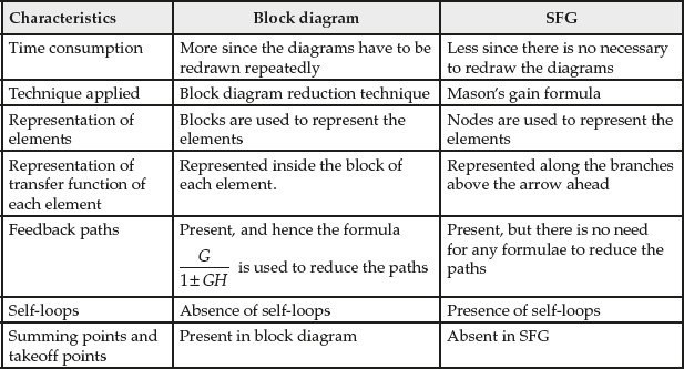
4.1.6 Comparison between SFG and Block Diagram

The comparison between SFG and block diagram based on certain characteristics is given in Table 4.3.

Table 4.3 ∣ SFG vs block diagram

Review Questions

1. Define signal flow graph of a system.
2. What are the terminologies used in a signal flow graph of the system?
3. Define a node.
4. What are the different types of nodes present in a signal flow graph representation of a system?
5. Define different types of node present in the SFG of the system.
6. Define a path.
7. What are the different types of paths?
8. Define different types of paths present in SFG of the system.
9. Define self-loop and non-touching loops.
10. Define gain.
11. What are the different types of gains?
12. Define forward-path gain and loop gain/feedback path gain.
13. What are the properties of a signal flow graph?
14. What do you mean by a signal flow graph algebra?
15. What are the rules for deriving the transfer function of a system using SFG?
16. Explain the different rules used in SFG of the system.
17. Define the following terms with reference to signal flow graphs: path, input node, sink, path gain, and loop gain.
18. Write down the Mason's gain formula for signal flow graph. Give the meaning for each symbol.
19. Explain with a neat flow chart, the procedure for deriving the SFG from a differential equation.
20. Compare block diagram with SFG technique.
21. The block diagram for a particular system is shown in Fig. Q4.21. (i) Obtain the SFG equivalent to the block diagram and (ii) determine the transfer ­function of the system using Mason's gain formula.
    

    Fig. Q4.21

22. The block diagram representation of a system is shown in Fig. Q4.22. (i) Obtain the transfer function using block diagram reduction technique and (ii) verify the result obtained using SFG.
    

    Fig. Q4.22

23. The block diagram for a particular system is shown in Fig. Q4.23. (i) Obtain the SFG equivalent to the block diagram and (ii) determine the transfer function of the system using Mason's gain formula.
    

    Fig. Q4.23

24. The block diagram for a particular system is shown in Fig. Q4.24. (i) Obtain the SFG equivalent to the block diagram and (ii) determine the transfer function of the system using Mason's gain formula.
    

    Fig. Q4.24

25. For the SFG of a system shown in Fig. Q4.25, obtain the transfer function of the system represented by SFG using Mason's gain formula.
    

    Fig. Q4.25

26. The SFG for a particular system is shown in Fig. Q4.26. Determine the transfer function of the system using Mason's gain formula.
    

    Fig. Q4.26

27. The SFG of a system is shown in Fig. Q4.27, obtain the transfer function of the given SFG using Mason's gain formula.
    

    Fig. Q4.27

28. The signal flow diagram for a particular system is shown in Fig. Q4.28. Determine the transfer function of the system using Mason's gain formula.
    

    Fig. Q4.28

29. For the SFG of a system shown in Fig. Q4.29, obtain the transfer function of the system represented by SFG using Mason's gain formula.
    

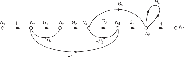
    Fig. Q4.29

30. The SFG for a system is shown in Fig. Q4.30. Obtain the transfer function of the given SFG using Mason's gain formula.
    

    Fig. Q4.30

31. The SFG for a system is shown in Fig. Q4.31. Obtain the transfer function of the given SFG using Mason's gain formula.
    

    Fig. Q4.31

32. The SFG for a system is shown in Fig. Q4.32. Obtain the transfer function of the given SFG using Mason's gain formula.
    

    Fig. Q4.32

33. The block diagram for a particular system is shown in Fig. Q4.33. (i) Obtain the SFG equivalent to the block diagram and (ii) determine the transfer ­function of the system using Mason's gain formula.
    

    Fig. Q4.33

34. The block diagram for a particular system is shown in Fig. Q4.34. (i) Obtain the SFG equivalent to the block diagram and (ii) determine the transfer ­function of the system using Mason's gain formula.
    

    Fig. Q4.34

35. The block diagram of the system is shown in Fig. Q4.35. Determine the transfer function by using block diagram reduction technique and verify it using SFG technique.
    

    Fig. Q4.35

36. The SFG for a system is shown in Fig. Q4.36. Obtain the transfer function of the system represented by SFG using Mason's gain formula.
    

    Fig. Q4.36

37. The SFG for a system is shown in Fig. Q4.37. Obtain the transfer function of the system represented by SFG using Mason's gain formula.
    

    Fig. Q4.37

38. The SFG for a system is shown in Fig. Q4.38. Obtain the transfer function of the system represented by SFG using Mason's gain formula.
    

    Fig. Q4.38

39. The SFG for a system is shown in Fig. Q4.39. Obtain the transfer function of the system represented by SFG using Mason's gain formula.
    

    Fig. Q4.39

40. The SFG for a system is shown in Fig. Q4.40. Obtain the transfer function of the system represented by SFG using Mason's gain formula.
    

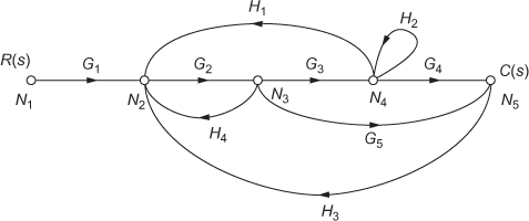
    Fig. Q4.40

41. For the SFG system shown in Fig. Q4.41, obtain the transfer function of the given SFG using Mason's gain formula.
    

    Fig. Q4.41

42. The SFG for a system is shown in Fig. Q4.42. Obtain the transfer function of the system represented by SFG using Mason's gain formula.
    

    Fig. Q4.42

43. The block diagram for a particular system is shown in Fig. Q4.43. (i) Obtain the SFG equivalent to the block diagram and (ii) determine the transfer function of the system using Mason's gain formula.
    

    Fig. Q4.43

44. The SFG for a system is shown in Fig. Q4.44. Obtain the transfer function of the system represented by SFG using Mason's gain formula.
    

    Fig. Q4.44

45. The SFG for a system is shown in Fig. Q4.45, obtain the transfer function of the system represented by SFG using Mason's gain formula.
    

    Fig. Q4.45

46. The SFG for a system is shown in Fig. Q4.46. Obtain the transfer ­function of the system represented by SFG using Mason's gain formula.
    

    Fig. Q4.46

47. The SFG for a system is shown in Fig. Q4.47. (i) Obtain the transfer function of the system using Mason's gain formula; (ii) draw its equivalent block diagram and verify the transfer function obtained.
    

    Fig. Q4.47

48. The block diagram for a particular system is shown in Fig. Q4.48. (i) Obtain the SFG equivalent to the block diagram and (ii) determine the transfer function of the system using Mason's gain formula.
    

    Fig. Q4.48

49. The SFG for a system is shown in Fig. Q4.49. Obtain the transfer function of the system represented by SFG using Mason's gain formula.
    

    Fig. Q4.49

50. For the electrical circuit shown in Fig. Q4.50, determine the transfer function of the system, using Mason's gain formula.
    

    Fig. Q4.50