
CONTENTS
15.2 Mechanism of Heat Transfer in Soil
15.3 External Thermal Environment
15.4 Native Soil Thermal Resistivity
15.5 Seasonal Temperature Changes at Operating Depth
15.11 Use of Corrective Thermal Backfills
15.12 Corrective Thermal Backfills
15.12.1 Compacted Granular Backfills
15.12.4 Fluidized Thermal Backfills (FTB)
15.13.1 Concrete for Cable Backfill
15.13.2 Florida Test Installation
15.14 Earth Interface Temperature
15.15 Elements of a Route Thermal Survey
15.15.5 Corrective Thermal Backfill and Thermal Stability
The determination of the ampacity of electric power cables has been discussed in Chapter 14. In that chapter, considerable emphasize has been placed on the “internal” aspects of the cable and the generation of heat inside the cable. This chapter will emphasize the external heat flow considerations that are required to carry the internal heat to the ultimate heat sink, the ambient earth’s surface.
The first practical calculation of the temperature rise in the earth portion of a cable circuit was presented by Dr. A. E. Kennelly in 1893 [2]. His work was not fully appreciated until Neher and Mr. Grath [23] demonstrated the adaptability of Kennelly’s method to cable engineering. As early as 1949, Jack Neher described the patterns of isotherms surrounding buried cables and showed that they were eccentric circles offset down from the axis of the cable [3]. This was later reported in detail by Balaska, McKean, and Merrell after they ran load tests on simulated pipe cables in a sandy area in New York [9]. They reported very high resistivity sand adjacent to the pipes. Analyses of the thermal resistivity of soils by Sinclair [3], Adams and Baljet [4], Black and Martin [5], and others have clearly shown that migration of moisture from the backfill soil is a critical element in the ampacity of cable systems [8]. Although a moisture content value per se is not a part of the ampacity calculation, it has the highest impact on the thermal resistivity of soil.
In-situ tests to determine the thermal resistivity of the native soil can be conducted by thermal needle method. IEEE Guide 442 outlines this procedure. Black and Martin have recorded many of the practical aspects of these measurements in reference [5].
15.2 MECHANISM OF HEAT TRANSFER IN SOIL
Heat flows through a soil primarily by conduction through mineral particles, and secondarily by conduction and convection through the moisture or air that occupies the pore space between solid particles. Thermal resistivity depends on soil composition and texture, water content, density, and various other factors to a lesser degree. This complex interrelationship does not lend itself to a simple formula; rather testing must be carried out on any given soil to determine its resistivity. Note that once a cable is installed, the soil moisture is the only parameter that changes significantly with time.
There are many factors that affect the thermal resistivity of soils:
1. Soil Composition
a. Mineral type and content
b. Organic content
c. Chemical bonding between particles
2. Texture
a. Grain size distribution
b. Grain shape
3. Water/Moisture Content
a. Degree of saturation
b. Porosity
4. Dry Density
a. Porosity
b. Solid content
c. Inter particle contacts
d. Pore size distribution
5. Ambient Temperature
6. Other Factors
a. Dissolved salts and minerals
b. Changes in water levels
Soil is a composite consisting of solid mineral grains, typically making point-to-point contact, and pore space filled with water and air. The thermal resistivity of a given soil mass is a function of the intrinsic resistivities of its components. These may range from 12°C-cm/W for quartz mineral, to 40°C-cm/W for limestone, to 165°C-cm/W for water, to about 500°C-cm/W for organics (Table 15.1). Even certain highly compacted soils can have up to 30% voids between solid particles, which in a dry state are filled with very high resistivity air (about 4,500°C-cm/W).
Quartz is three to five times more conductive than other minerals. Reactive clay minerals enhance particle bonding; flaky mica particles can be indicative of a loose microstructure. In addition, grain shape (round, elongated, platy) and angularity influence soil density, grain contacts, and microstructure. A significant organic content (say >4%) can substantially increase resistivity.
Soil texture refers to the soil grain size, shape, and particle size gradation. Since most of the heat conduction is through the solid particles and their contacts, the resistivity is minimized for soils that maximize these contacts—Figure 15.2. Well-graded materials and those consisting of crushed particles (i.e., angular as opposed to rounded or uniform grains—Figure 15.1) generally have more particle contacts and compact to higher densities. This has the added benefit of retarding moisture migration because of the smaller pore spaces. To ensure backfill thermal performance, particle gradation limits are specified based on a sieve analysis.
Material |
Thermal Resistivity |
Quartz, Silica |
12 |
Granite |
30 |
Limestone |
40 |
Sandstone |
50 |
Shale |
60 |
Shale (friable) |
200 |
Mica |
170 |
Ice |
45 |
Water |
165 |
Organics |
~500 |
Air |
~4,500 |
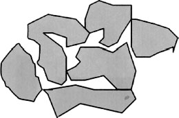
FIGURE 15.1 High thermal resistivity soil (low density and high porosity).
In a wet soil, water provides an easy path for heat conduction over these thermal bridges. As the soil dries, discontinuities develop in the heat conduction path and the thermal resistivity increases.
Densification increases mineral grain contacts and displaces air (i.e., lowers the porosity), thereby reducing the soil resistivity, most notably at low moisture contents. Well-graded soils are potentially denser because smaller grains can efficiently fill the spaces between the larger particles (Figure 15.2). The specification of a minimum dry density for a corrective thermal backfill is one factor in obtaining the required thermal performance.
For a given soil, the major influence on the thermal resistivity is the moisture content. In a dry state, the pore spaces are filled with air (~4,500°C-cm/W); thus extremely restricted heat conduction paths exist only along the mineral contacts. As water (~165°C-cm/W) replaces air, the soil resistivity is substantially lowered (as much as three to eight times) as the relatively good heat conduction paths are expanded (thermal bridges, Figure 15.3). This is illustrated by the thermal dryout curve (thermal resistivity vs. soil moisture content, Figure 15.4). A soil that is better able to retain its moisture, as well as able to efficiently re-wet when dried, will have better thermal performance characteristics.
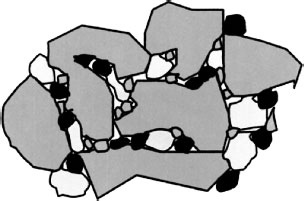
FIGURE 15.2 Low thermal resistivity soil (higher density and lower porosity).
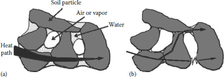
FIGURE 15.3 Influence of water (moisture content) on thermal resistivity. (a) Wet soil: high water content provides an easy path for heat conduction (“thermal bridges”), therefore the soil thermal resistivity is low. (b) Damp soil: as soil dries, discontinuities develop in the heat conduction path due to low water content, therefore themal resistivity increases.
Cables that are installed under the groundwater table will experience a constant and low soil thermal resistivity; but, if the water table should ever drop below the cable level, then the potential for thermal drying of the soil and attendant high thermal resistivity exist. Below the groundwater table, thermal stability is generally not a problem, although some drying may occur in very clayey soils under an extended application of an excessive cable heat load.
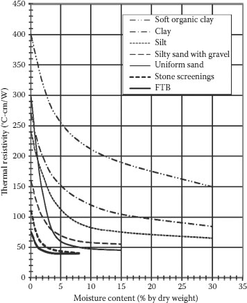
FIGURE 15.4 Impact of moisture on ampacity.
Above the water table, the ambient soil moisture varies with the seasons. The thermal resistivity should be assessed at the driest expected conditions.
For a native soil, the dry density does not change with time, but spatially, a soil of the same composition and moisture content may exist at different densities; or it may be backfilled at a density different from the natural condition.
At higher soil moistures, the thermal dryout curve is relatively flat. At lower moistures, the curve slopes upward more steeply, such that a small amount of soil drying gives rise to a larger increase in thermal resistivity. The critical moisture is defined as the point below which the thermal resistivity begins to increase disproportionately. Well-graded and granular soils have a sharp knee in their thermal dryout curves and the critical moisture is clearly defined (Figure 15.4). For these soils, as a rule, the critical moisture may be taken at the point where the wet (flat line) thermal resistivity has increased by 10%.
The critical moisture is not so evident for the gradually sloping curve of fine grained soils and becomes a more subjective choice; for these soils, the Atterberg plastic limit/ASTM D4318 is a good indicator of the critical moisture.
Intuitively this makes sense, since the plastic limit is the lowest moisture at which the soil is malleable. It no longer contains “free” gravitational water and at lower moistures begins to crumble when handled. Thermally this limit corresponds to the breakdown of the moisture thermal bridges; therefore, it follows that below the plastic limit, the thermal resistivity should begin to increase proportionally more.
15.3 EXTERNAL THERMAL ENVIRONMENT
In simple terms, a cable can be considered as the “heat source” and the earth’s surface as the “heat sink.” All the heat generated by a cable must reach the earth’s surface through the external thermal environment of the cable. This may consist of a corrective thermal backfill surrounding the cable, the native soil, and other materials. Installations in urban areas may consist of “road base,” concrete and asphalt. Some of these materials and the thickness of the layers may be defined (regulated) by other agencies such as department of transportation (DOT) and local municipalities. For all practical purpose, the mechanism of heat transfer from underground cables is by conduction and therefore each layer and its thermal resistivity will impact the cable rating.
In order to calculate the ampacity of any underground cable, it is necessary to know the
1. Soil thermal characteristics
2. Earth ambient temperature at burial depth
3. Surface or air temperature
15.4 NATIVE SOIL THERMAL RESISTIVITY
An aspect that must be considered is the long-term stability of the soil during the heating process. Heat tends to force moisture out of soils, increasing their resistivity substantially over the soil in its native, undisturbed environment. This means that measuring the soil resistivity prior to the cable carrying load current can result in an optimistically low value. Therefore, it is essential to conduct “thermal dryout characterization” of the soil and that of the backfill. An appropriate value of the thermal resistivity is determined from this dryout curve. Factors that affect the drying rate and thermal stability will be discussed.
Common components of soils with their thermal resistance (rho) in °C-cm/watts are shown in Table 15.1. The values for water and air are based on conduction—not for moving air or water.
The earth that surrounds a cable system can have great variations in thermal resistance along its route. This can be the result of natural soil variations as well as moisture migration caused by heat produced current flow. The backfill material that surrounds a cable system is an extremely critical element in achieving optimum heat dissipation of the system.
Along a cable route, the native soil thermal resistivity can vary significantly as a function of the distance and also of depth. In addition, these values can change from, say, 50°C-cm/W–60°C-cm/W at a moisture content of 10% to, say, about 150°C-cm/W at 10% and as high as 350°C-cm/W in totally dry condition (0% moisture content) (Figure 15.4).
Organic soils such as “peat” and “top soil” or soils with vegetation or root matter exhibit high thermal resistivity, both in wet and especially in dry condition. These type of soils have relatively high moisture content but fairly low density. They are very porous (permeable) and therefore will dry relatively easily. The high porosity results in high voids (air content) and thus very high resistivity. If native soil is considered to be used as a nonclassified backfill over a good quality “corrective thermal backfill envelope” or over a “concrete duct-bank,” it must be free of all organic matter.
The impact of soil thermal resistivity on ampacity of cables directly buried in a native soil is shown in Figure 15.5. While actual values for rho and amperes vary widely, this relationship holds for any cable system, regardless of the voltage. The change in the soil thermal characteristic (primarily the thermal resistivity) is purely a function of the heat output of an energized cable system and not the voltage. A low voltage cable system may have numerous cables in a single trench or only a few cables carrying very high current. The resultant net heat output per unit length of the trench is the prime factor that induces the soil moisture migration (drying) that results in higher thermal resistivity.
On wind and solar farm projects, the cables are operated at relatively low voltages (34 kV). However, the risk of cable failure is quite high if the native soil that is used to backfill the trenches is not installed at the specified density in order to meet the design thermal resistivity.
The effective thermal resistivity of a combination of imported backfill and the native soil surrounding a trench is shown in Figure 15.6. Optimized thermal characteristics and dimensions of the envelope of the controlled backfill around the cable will produce a lower effective thermal resistivity. Most computer-based ampacity programs are capable of handling the numerous variables and parameters for such situations.
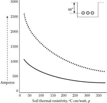
FIGURE 15.5 Effect of soil thermal resistivity on ampacity.
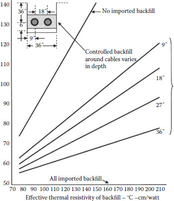
FIGURE 15.6 Effective thermal resistivity.
15.5 SEASONAL TEMPERATURE CHANGES AT OPERATING DEPTH
Another important factor that influences the ampacity of a cable is that earth temperatures change with depth. Ground temperature changes on a seasonal basis, following the air temperature but with a much reduced amplitude. The soil temperature varies significantly in the top 3 ft (1 m) and the variation decreases rapidly with the depth as indicated by the typical curves in Figure 15.7. Temperatures are quite constant below 4 m (13 ft) depth. Also there is a time lag between the maximum air temperature and the maximum soil temperature at a given depth. Local data is available from government environment, weather, and agriculture agencies.
Thermal stability is a concept used to describe the ability of a moist soil to maintain a relatively constant thermal resistivity when subjected to an imposed heat load, thus allowing a power cable not to exceed a safe operating temperature. Thermal instability (or thermal runaway) occurs when a soil is unable to sustain the heat from a cable and the soil progressively dries resulting in a substantial increase in the soil thermal resistivity and attendant increase in the cable operating temperature. If moisture is not replenished or current reduced, the ultimate result may be cable failure due to overheating.
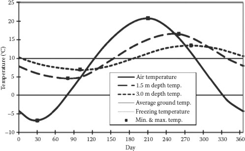
FIGURE 15.7 Seasonal temperature change with depth.
Heat flow through a moist soil takes place predominantly by conduction. At high moisture levels, liquid fills the gaps between soil particles and provides a continuous medium, which makes an efficient thermal conductor (Figure 15.3). When an appreciable heat rate is emitted by a heat source, there is a tendency for the liquid to vaporize near the heat source and to condense in the cooler regions away from it (moisture migration). On the other hand, there is significant liquid return flow by capillary suction, which tends to maintain a balanced liquid moisture distribution throughout the soil (thermal stability—region A in Figure 15.3).
If the amount of liquid drops below the critical moisture content, then the imposed heat causes the liquid thermal bridges between the soil particles to break down more rapidly than the capillary suction can replace them. This in turn increases the thermal gradient in the soil, forcing more moisture migration, resulting in a significant increase in the thermal resistivity around the heat source (thermal instability—region B in Figure 15.3).
The heat transfer rate at the cable–soil interface is the driving force tending to cause moisture migration in the soil. Depending on the soil type and moisture conditions, a minimum heat rate must be exceeded before thermal instability conditions can arise. Larger diameter cables may not promote moisture migration as they dissipate heat over a larger surface area. That is, although a thermal probe, single-conductor cable, or pipe-type cable, may generate the same heat rate (watts per centimeter), the heat flux or watts density (watts per centimeter squared) at the soil interface is less for the larger diameter. The effective diameter is the diameter of an individual cable for directly buried cables and the pipe or conduit diameter for pipe-type cables or cables in ducts. Depending on the arrangement, the individual cable heat rate for a multicable system may be increased because of the mutual heating effect. As a worst case, the heat rate impinging on the soil can be taken as the sum of the individual heat rates.
A thermally stable backfill placed around a cable effectively moves the critical cable–soil interface outward to the backfill–soil interface. Thus, the native soil experiences a greatly reduced heat flux that will not cause it to become thermally unstable.
Stability is also a function of the cable loading history. Although a steady application of a heat rate may eventually dry a soil, load cycling may allow time for the soil to replenish lost moisture, delaying or negating the onset of instability. Emergency loadings tend to dry the soil near the cable, but the duration is generally not long enough to do much damage. Thermal stability testing can indicate a safe length of time for emergency loadings for a given cable–soil system.
Thermal stability is not a function of cable temperature. Rather, the temperature is an effect of the cable heat–soil resistance interaction. Previously, ampacity tables had been developed based on allowable cable interface temperatures, since these temperatures were an easy thing to measure. This concept is incomplete since it does not consider different soil types, moisture variations, or the dynamic nature of the soil thermal resistivity. The ampacity tables may have generally provided safe cable designs and operations only because of a high degree of conservatism.
Certain soils and soil conditions enhance the thermal stability of a cable system. A soil must be an efficient heat conductor and have the ability to resist moisture migration when subjected to a heat load, as well as re-wet quickly if dried. This is best accomplished with a well-graded sand to fine gravel (sound mineral aggregate), with a small percentage of fines (silt and clay), that can be easily compacted to a high density. For maximum density, the smaller grains efficiently fill the spaces between the larger particles, and the fines enhance the moisture retention. A sound mineral aggregate, without organics, and without porous or friable particles, ensures efficient thermal conduction. Porous soils will dry quickly and therefore they are unstable; although a clayey soil dries very slowly, it cannot be easily re-wetted and therefore it is also a poor soil.
Above the water table, the natural soil moisture content is not constant but varies in response to climatic conditions. In the operation of a cable, the soil has the greatest potential for induced instability when it is in its driest state. At this point, the added heat load from a cable may create an unstable situation. The stability of a soil must be assessed at its lowest expected ambient moisture content; but this is frequently not an easy parameter to determine.
Figure 15.8 indicates a typical temperature–log time response of a thermal probe inserted in a moist soil and emitting an appreciable heat rate. The slope of the initial straight line is proportional to the thermal resistivity of the moist, thermally stable soil. When sufficient moisture migration has taken place to cause a substantial drying of the soil (critical moisture content), the line begins to curve upward. This point, called the initial drying time, is the onset of thermal instability. Further heating will result in rapidly increasing resistivity and the complete drying of the soil around the probe, as indicated by the final straight line portion of the curve, whose slope is proportional to the resistivity of the dry soil.
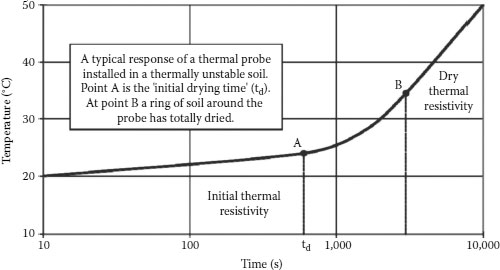
FIGURE 15.8 Thermal stability limit.
Analytically the initial drying times for different diameter heat sources dissipating the same constant heat rate (watts per centimeter), in identical soils, are related by the ratio of the diameters squared (the Fourier number). Thus, the initial drying time determined in the laboratory using a small diameter thermal probe can be extrapolated to the initial drying time for a large diameter, operating underground power cable:
The parameter t/d2, called the thermal stability limit, is a constant and depends only on the heat rate and initial moisture content for a given soil. Test results are presented as a plot of heat rate vs. thermal stability limit for a range of initial moistures (Figure 15.9).
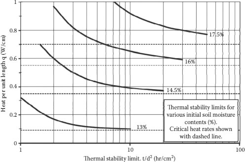
FIGURE 15.9 Thermal stability limits for various initial moisture contents.
The initial drying time is a conservative estimate of the time to instability for an installed cable. First, it assumes the constant application of the full heat load, when in fact an operating system is subjected to load cycles. Second, it only indicates when an unstable condition first appears, but a cable would not experience significant heating for some time. Third, it assumes no moisture replenishment, which could occur in the field. Overall, though, a conservative estimate of the drying time may be a reasonable, safe value to use to calculate the thermal stability limit, since the lowest expected ambient soil moisture content is not usually well known and may be less than the initial moisture contents chosen for the tests.
The analytical model also predicts the existence of a limiting heat rate. This is indicated by the asymptotes of the empirical curves in Figure 15.9. Below the critical heat rate, a poor thermal soil will remain stable for an essentially indefinite period of time.
Once a drying time has been determined in the laboratory and extrapolated for the cable, a soil can be considered stable if:
1. The drying time exceeds the longest expected drought.
2. The cable loading is below the critical heat rate for a substantial time, particularly when the soil is driest.
A search for a local source of an ideally graded, natural soil often proves difficult. Native soils frequently have a rather uniform size and hence dry out very quickly when a heat source is applied. Typical silica sand has 88% of the sand passing through a #40 sieve (0.42 mm or smaller) and with 0.6% silt. Dry densities of only about 100 pounds per cubic foot, mostly made of quartz crystals that have a thermal resistivity of about 12, are attainable with normal construction techniques. The thermal resistivity of these sands in their native state is about 60 to 80 rho as long as they have about 3% by weight of moisture. Typically, a load of about 30 watts per foot from a cable or duct bank is sufficient to dry such sand to less than 1% moisture where the rho can rise to 350–400.
Thermal runaway conditions of native soils have been experienced by many utilities involving transmission cables as well as single-circuit, direct buried distribution feeder cables. In one situation, the sand had less than half percent moisture adjacent to a direct buried feeder cable exiting a substation even though lawn irrigation sprinklers were only 2 ft above. With 4 hours of watering every night, the sand could not retain enough moisture to prevent thermal runaway of a buried three-conductor 500 kcmil copper feeder cable. The pattern of eccentric circles of dry sand was found to be in agreement with the paper of Balaska, Merrell, and McKean [9], which described a simulated transmission cable in a sand hill in New York.
In another example, the native soil around a pipe cable was found to be baked completely dry and adhering to the pipe’s outer surface even though the cable was 30 ft under the surface of a bay. The material in this situation had a clay-like composition (marl) with a high amount of organic fillers.
Similar reports have been given regarding high thermal resistivity of soils around cables under waterways in Denmark, England [10], and the deepest water in Lake Champlain [11].
In the situation described in Denmark, it was stated that “Cooling conditions for a submarine cable are normally assumed to be very good and the ampacity is based on a low value of thermal resistivity of the seabed.” Since the land section had a thermal resistivity of 43°C-cm/watt to 54°C-cm/watt, it was assumed that the value in the seabed was equally as low. After two joints failed in service, it was discovered in laboratory investigations that the seabed material contained high organic levels and that the thermal resistivity was 105°C-cm/watt. Needle probes into the seabed discovered a rho of 94°C-cm/watt.
In the London investigation [10], they found the silt in the bottom of canals to be as high as 118°C-cm/watt and that even higher values could be reached in the presence of heated cables.
The Lake Champlain 115 kV cables [11] were installed in 1958 and failed in 1969 at a depth of about 300 ft. A sample of the soil near the site of failure was sent to a laboratory for analysis. They found the silt to have an average value of rho of 90 to 100 even though the silt “was not tested in the condition that it was in the lake bottom….” The new cable rating was based on the lakebed silt to have a rho of 140°C-cm/watt.
The lesson to be learned here is that moisture can migrate from soils even in deep waterways. To maintain a low thermal resistivity soil in a seabed, water must be free to move through a porous or granular environment and have a limited level of organic material. It should also be pointed out that readings taken with thermal probes along a proposed route may give optimistically low values of thermal resistivity if the heat source is not left on long enough to detect moisture migration in that soil.
The thermal dryout curve of a good thermal soil has a sharp knee at low moisture content and thus the critical moisture can be clearly defined; also, the totally dry thermal resistivity is quite low. Furthermore, above the critical moisture the thermal dryout curve is quite flat, that is, the resistivity is fairly constant and relatively independent of the soil moisture (i.e., crushed stone screenings in Figure 15.4). For these soils the thermal stability may be treated as a simple “binary” concept that is, above the critical moisture content the soil is stable (fairly constant resistivity), whereas below this moisture it is unstable (rapidly increasing resistivity). In the thermally stable range, an imposed heat rate causes a local redistribution of the moisture but an equilibrium between vapor outflow and liquid return is established leaving the resistivity virtually unchanged because of the flat nature of the thermal dryout curve.
In a cable installation, good thermal soil should be placed next to the cable, therefore, under normal heat loads, the simple concept of critical moisture can be used as the indication of the thermal stability. For these backfills, above the critical moisture, realistic cable heat loads do not exceed the critical heat rate as this would result in very long drying times (in the order of months). An exceptional heat load, though, may cause a stable situation to become unstable. In this case the drying time test, as previously discussed, may also be carried out for the good thermal backfill.
Thus, if the lowest expected ambient soil moisture is above the critical moisture, then the good thermal soil may be considered to be stable, and the lowest expected ambient soil moisture is used to determine the design thermal resistivity from the thermal dryout curve. If the lowest expected moisture content is below the critical moisture, then an unstable condition exists and the totally dry thermal resistivity must be used for the design. For a good thermal soil, though, the dry resistivity is still quite reasonable for cable operation.
For clayey soils, the thermal resistivity increases fairly steadily as the moisture decreases without a definite critical moisture (Figure 15.4). For these fine grained soils, moisture movement is a slow, continuous process because of the extremely low permeability of the liquid phase. Therefore, a liquid–vapor equilibrium is not attained in a short-term thermal loading, and for these poor thermal soils the question is one of the time required for a substantial increase in thermal resistivity for a given heat rate.
Even though a uniform sandy soil (Ottawa sand in Figure 15.4) has a fairly constant and low thermal resistivity above the critical moisture, it is a poor thermal soil because of the high dry resistivity. For these porous soils, moisture movement and drying take place very easily, and large moisture redistribution above the critical moisture is likely.
The drying time concept must be used if one wishes to analyze the thermal stability of poor thermal soils.
15.11 USE OF CORRECTIVE THERMAL BACKFILLS
Invariably, native soils do not make good thermal backfills because their thermal performance is poor, or they are difficult to backfill properly. In its natural state a native soil may exhibit the thermal dryout curve of a good thermal soil. But, if the native soil does not have the correct texture or moisture content, once it is excavated it is difficult to handle and re-compact efficiently, and a poor thermal dryout curve may result. Also contamination with topsoil and other organic soils is difficult to avoid. Importing a corrective thermal backfill, with its assured excellent thermal performance, may not be much more expensive than attempting to use a marginal native soil. In the long run, the operational reliability gained by placing a classified thermal backfill around the cable has advantages over the possible variability and uncertainty of re-compacted native soil.
The common practice has been to use granular bedding material around a cable. In the past, fairly uniform sands that may compact well but have a poor thermal performance have been used. Only a good thermal backfill is to be placed around the cable (Section 15.10). The thickness of the backfill envelope should be such that the heat flux impinging on the native soil is so low as to be inconsequential for instability considerations. Now only the thermal stability of the backfill must be considered, which can be established by applying the binary concept.
15.12 CORRECTIVE THERMAL BACKFILLS
The use of a well-designed corrective thermal backfill can significantly enhance the heat dissipation and increase the ampacity of an underground power cable, as well as alleviate thermal instability concerns. The corrective backfill will reduce the heat flux experienced by the native soil so that it will not dry out. A good backfill should be better able to resist total drying and also have a low dry resistivity if it is completely dried. Typically, a trench is filled with thermal backfill to a minimum height of 300 mm above the cable. If poor quality native soils are encountered along a route, the thickness of the backfill can be increased to maintain a low composite resistivity.
Generally, utilities have relied upon the suppliers of such backfill materials to meet acceptable thermal and mechanical performance characteristics. Very few utilities have set stringent specifications or have a quality assurance program for installed backfills, especially with respect to thermal performance. The extra cost involved in the use of a properly designed and installed thermal backfill is somewhat higher than that involved in the use of unclassified material (i.e., native soils, bedding sands), yet cable rating increases are significant and can amount to substantial revenue gains for a utility over the life of a cable. It is usually not cost-effective to modify the native soil by using additives to improve its thermal properties.
Placing corrective thermal backfill in a cable trench will reduce the effects of high native soil resistivities. A constant composite resistivity can be maintained along the whole cable route by adjusting the thickness of Fluidized Thermal Backfills™ (FTB) to balance the variations in the native soil resistivity. Other factors, such as trench dimensions, cable spacing, burial depth, ambient conditions, etc., should also be taken into account for optimum design. This can easily be done using computerized cable ampacity programs.
It is important to note that the adverse effects of poorly constituted or installed thermal backfills are not reflected in the performance of the cable system in the early stages when the loads may be low. However, temperatures may rise beyond allowable levels as the loadings increase. The remedial cost of removal and replacement of such backfills is very high, especially if the area is paved. On the other hand, the loss of revenues from de-rating a system may be even higher.
Generally, native soils do not make good thermal backfills because their thermal performance is poor, or they are difficult to properly re-compact in a cable trench. In its natural state, a native soil may exhibit the thermal dryout curve of a good thermal soil. But, if the soil does not have the correct texture or moisture content and once it is excavated, it is difficult to handle and re-compact efficiently (especially clayey soils), and a poor thermal dryout curve may result. Also, contamination with topsoil and other organic soils is difficult to avoid. Importing a corrective thermal backfill, with its assured excellent thermal performance, may not be much more expensive than attempting to use a marginal native soil. In the long run, the operational reliability gained by placing a classified thermal backfill around the cable has advantages over the possible variability and uncertainty of re-compacted native soil.
15.12.1 COMPACTED GRANULAR BACKFILLS
Over the years, many unsuitable sands have been used as thermal backfills (so called “thermal sands”) because of the ease of installation. Almost any sand, when moist, will give a reasonably low resistivity. The crucial aspect is its thermal performance when subjected to cable heat loads and when partially or totally dried. Uniform bedding sands dry easily and can have dry thermal resistivities exceeding 250°C-cm/W.
Since most of the heat conduction is through the soil mineral particles and their contacts, one must ensure a soil mixture that maximizes these contacts, that is, a high density soil. Well-graded soils are denser because smaller grains can efficiently fill the spaces between the larger particles. A good thermal backfill is specified by a narrow range of gradings based on a sieve analysis, and should have a wet thermal resistivity of 35°C-cm/W to 50°C-cm/W and a dry resistivity of 90°C-cm/W to 120°C-cm/W.
For a given soil, the major influence on the resistivity is the moisture content. A soil that is better able to retain its moisture, as well as able to efficiently re-wet when dried, will have a better thermal performance. A small amount of very fine particles (i.e., silt and clay size) or cement enhances this property.
It is easy to conclude that, in general, a well-graded sand to fine gravel (sound mineral aggregate), free of organics, and with a small percentage of fines, would make an ideal thermal backfill when compacted to its maximum density. Some natural sands may be suitable, although they must often be blended, which can be costly. Most crushed stone screenings meet these gradation characteristics, but the sharpness of the stone chips may cause concerns about damage to cable insulation. For a specific backfill, the laboratory determination of an optimum standard Proctor density and moisture and thermal dryout curve are essential to confirm its thermal performance.
The addition of a binder can improve the thermal performance of a poorly graded sand. Thorough mixing and proper compaction are crucial to the performance. A small quantity of cement (~2%) enhances the resistivity and stability of granular backfills. The addition of chemical, wax, or latex binders has also been suggested. Although the thermal properties are improved, field application is not practical. They are expensive and difficult to handle and transport, as well as being environmentally incompatible. Basically, cement is the only practical binder that should be considered.
One often neglected factor about compacted backfills is the need for quality assurance during installation. If the gradation of the backfill is not correct, or it is not at the optimum moisture content, or not enough compaction effort is applied, or the backfill lifts are too thick, then the maximum density will not be achieved and the thermal performance is degraded. This is especially significant in the restricted areas around cable groups where proper compaction is very difficult. Yet it is precisely in these zones, adjacent to the cables, that proper compaction is most important to ensure maximum heat dissipation from the cables.
A classified granular soil (i.e., specified grading and mineral quality) is more expensive than unclassified pit-run material. The transportation cost, though, is the prime factor in the site delivered cost and therefore suppliers should be as close as possible to the project site. The installation and quality assurance costs must be added to the material and transportation costs to arrive at the final cost. When compared on a final cost basis, it may be less expensive to use an FTB.
Corrective backfills must meet several criteria, including thermal efficiency and engineering performance compatible with road base material (mechanical support, no settlement, resistance to erosion, and frost heave). The backfill is specified by a gradation of grain sizes and a dry density. Proper installation of a granular backfill is crucial in meeting the above criteria.
A granular backfill reaches a maximum density at a specific optimum moisture content; at higher or lower moistures a lower density is attained. This behavior is indicated by the standard Proctor laboratory test (Figure 15.10). Installation specifications for a particular material usually require that 95% of the maximum Proctor dry density be attained. In order to meet the required density, the contractor must use suitable compaction equipment, ensure optimum moisture, compact in thin lifts, and use several passes over the same area.
Compacting in thick lifts may be faster but it leaves low density fill material beneath a dense crust. This is why rigorous inspection is required. For smaller, trench-type compactors the lifts should not exceed 150 to 200 mm (6–8 inches), especially close to the cables where more care and effort are needed to ensure maximum density. Thicker lifts may be permitted as the backfill reaches the ground surface (Figure 15.10).
Usually, stock-piled backfill is not at the optimum moisture content. Generally, it is too dry and moisture must be mixed in or sprayed on each lift before compacting. For granular, noncohesive soils the optimum moisture is about 8% to 12% and the soil appears quite wet.
The commonly used trench compactors are plate vibrators, vibrating rollers, and dynamic impactors (jumping jacks). The vibratory types are better for granular soils while the impact types are more effective with clayey soils. The smaller hand operated compactors are preferred because they are easy to maneuver in narrow areas. Flooding and hydraulic filling will not yield the same result as backfill may segregate. Ramming or drop weights are not acceptable because of poor control and the possibility of damage to cables.
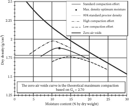
FIGURE 15.10 Soil compaction.
The corrective backfill may be sourced from several suppliers. From each supplier, a specific material is chosen based on mineral quality, sieve analysis, standard Proctor density, and thermal dryout curve. For field installation, a minimum density (or maximum thermal resistivity) is specified for the specific backfill. A field quality assurance program is a must; otherwise, there is no way of ascertaining that the performance specifications are met.
An experienced on-site inspector should be able to visually check the consistency and quality of the material supplied. Occasional sieve analyses (two or three times) will confirm the grading.
The inspector should monitor the backfill moisture, lift thickness, and thoroughness of compaction. Regular in-situ moisture and density tests should be performed (say, every 20 m along the trench), according to ASTM procedures, by an independent firm. Troxler nuclear density devices are commonly used. The level of back-scatter from a nuclear source can be related to density. Only certified personnel may use these devices. A sand cone method is still used. Standard sand is poured from a calibrated cone into a small hole dug in the backfill. The weight of the sand used can be related to a volume. The weight of the backfill removed divided by the volume is the density. If measured densities are significantly deficient, the backfill must be removed and re-compacted.
The thermal resistivity of the installed backfill may be tested periodically (say, every 100 m). If the backfill is compacted properly, then there should be no problem with the thermal properties. Preferably, an undisturbed Shelby tube sample should be obtained, which can be dried out in the laboratory to check the dry resistivity.
15.12.4 FLUIDIZED THERMAL BACKFILLS (FTB)
FTB is a material engineered to meet specific thermal resistivity, thermal stability, strength, and flow criteria, as well as to offer construction advantages. Such a free flowing, controlled density fill is ideally suited for hard-to-access areas such as narrow trenches, small diameter tunnels, or areas congested with many underground services—basically where mechanical compaction is neither feasible nor practical. In addition, although a compacted backfill may provide a good thermal envelope, it is a labor-intensive process that requires strict quality control. While the material cost of FTB may be high, it should even be considered for general usage because of its assured quality and performance standards and because it can be installed very quickly, thereby speeding up construction and decreasing overall costs.
Commonly available “controlled density fills,” “flowable fills,” or “slurry backfills,” which use large volumes of fly ash or sand, may meet the mechanical and flow requirements for trench backfilling, but they are completely unsuitable with respect to thermal performance. FTB should be designed and formulated by soil thermal specialists.
FTB is a slurry backfill consisting of a medium stone aggregate, sand, a small amount of cement for strength and particle bonding, water, and a fluidizing agent such as fly ash to impart a homogeneous fluid consistency. The component proportions are chosen, by laboratory testing of trial mixes, to minimize thermal resistivity and maximize flow without segregation of the components.
FTB will flow readily to fill all the voids, without vibration, yet harden quickly to a uniform density. Future settlements, if any, are negligible. It also affords mechanical protection for the cables and provides support for underground and surface facilities. FTB has good heat dissipation properties even when totally dry. Depending on the mix design, typical thermal resistivity values are 35°C-cm/W to 45°C-cm/W wet and 65°C-cm/W to 100°C-cm/W dry and thermal stability is excellent with a low critical moisture (less than 3%).
FTB is supplied as a ready-mix in concrete trucks and may be installed by pouring or pumping and usually does not require specific shoring or bulkheading. It solidifies by consolidation, with excess water seeping to the top. Pipes or ducts must be anchored or weighted down because of the buoyancy effect of the slurry. Regular FTB can be pumped up to 100 m, and greater distances with special modifications, using conventional concrete pumping equipment. Direct buried cables will not be damaged during installation, which may be a concern when using mechanical compaction devices. FTB solidifies quickly so that the ground surface may be reinstated the next day; but the low strength ~150 psi (1 MPa) affords easy “diggability” if the cables must be accessed in the future. If a higher strength is required, the cement content can be increased, and water adjusted, without degrading the thermal performance.
Quality control, during installation, is a matter of a few simple tests, such as random grain size analyses of the aggregates at the batch plant; air content (less than 2%) and slump (200 to 250 mm) measurements on the FTB before pouring. If the mix is too wet it must be rejected, therefore it may be ordered drier than required and water added at the site. Sample cylinders should be cast for strength, density, and thermal resistivity determinations in the laboratory when the FTB has hardened. For low strength FTB, two test cylinders for strength and two for resistivity should be cast for every 50 m of trench length. (Cylinders for high strength FTB tests should be cast as specified by ASTM for normal concrete.)
Normal strength ~3,000 psi (20 MPa) concrete (100 mm slump, nonair entrained) also has good thermal performance characteristics (less than 100°C-cm/W, totally dry). The addition of air, fly ash, or porous aggregate will increase the thermal resistivity. For general applications, though, it does not flow readily, is more expensive than FTB, and cannot be removed easily if access to the cables is required. It may be used in duct banks or where high strength is a structural requirement [1,7].
Lean mix concrete (i.e., less cement, about 0.5 MPa), with a slump of about 100 mm, does not have the superior flow characteristics of FTB, and has a higher thermal resistivity because the crushed stone and sand aggregate combination is not ideal. For installation around cables, it requires either vibration or light compaction. Adding water to enhance the flow will increase the voids content, thus raising the thermal resistivity, and in the worst case, may lead to segregation of the mix components. Chemical additives, to increase the flow, are only effective at higher cement contents. Additives such as fly ash or bentonite when used in small quantities in lean mix concretes will substantially increase the flow characteristics.
15.13.1 CONCRETE FOR CABLE BACKFILL
Cement bound sand (weak concrete) has been used as a backfill material around direct buried cables in Europe for many years. A typical material in use with a 12:1 sand/cement mix. Although this provides for some cable movement and relative ease for removal, these mixes do attain a rather high thermal resistivity when a load is applied for many months. A resistivity of about 105°C-cm/watt is typical. Lower values of rho may be attained by decreasing the ratio of sand to cement; in other words, by making the concrete more structurally sound.
Greebler and Barnett [12] reported that concrete around a laboratory installed duct bank had a rho of 85. This paper was the source of the 85 rho that may be found in the original “black books” of AIEE-IPCEA Ampacity Tables [6]. This concrete was poured above the floor in a wooden trough and was in an air conditioned building. This resulted in a poor structural cure and poor thermal resistivity. Brookes and Starr [13] found that the thermal resistivity of concrete around a buried pipe in New Jersey stayed at about 50 rho until the test was stopped after 24 months.
Nagley and Neese [14] found that the thermal resistivity of concrete around duct banks in the Chicago area varied from 38 to 53. An interesting discovery of their study was that a thin envelope of concrete around heavily loaded duct banks (about 1.25 inches rather than the more frequently used 2.5 inches) allowed the soil around the duct bank to dry out. The effective thermal resistivity of the surrounding earth soon reached unacceptably high levels.
The publication by the US Bureau of Reclamation in 1940, “Thermal Properties of Concrete,” [7] showed that the thermal resistivity of concrete used in the Boulder (now Hoover) Dam varied from 28.5 to 42.5.
15.13.2 FLORIDA TEST INSTALLATION
To determine the actual resistivity of locally available structural concrete, a test facility was constructed in Florida. Two 8 1/8 inch steel pipes, covered with 0.5 inches of Somastic, were placed one above the other in a trench with 12 inches of separation. This configuration was chosen since it would permit evaluation of the effects of burial depth as well as provide more information on a configuration that might be required in a restricted area.
Thermocouples were installed on the pipe in each section, on the Somastic, 3 and 6 inches from the Somastic, and under the earth 6 inches from the outer surface of the concrete envelope. Figure 15.11 shows the test arrangement.
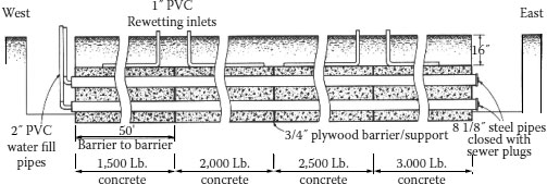
FIGURE 15.11 Arrangement of test envelope.
Four 50-foot sections were poured with various grades of commercially available structural grade concrete in a 6-inch envelope as shown in Figure 15.6. The compressive strengths of these four mixes were 1,500, 2,000, 2,500, and 3,000 pounds/in2. All sections were allowed to cure for 40 days prior to any application of heat to simulate normal cure in the earth.
The heat was increased from 15 to a high of 31 watts per foot in each pipe and continuing that load until the temperatures stabilized. Values of thermal resistivity were calculated for each pipe and its surrounding material separately by using Bauer’s version [15] of the Kennelly formula [2].
The thermal resistivity of the concrete varied throughout the test period, but the general trend was a slight decrease in resistivity for the three higher strength mixes. The section that had the 1,500 pound/in2 concrete was eliminated from the test after 3 months because the heater wires had burned out and the rho was increasing in that section (Table 15.2).
The 31 watts per foot level was chosen as the maximum because this resulted in an interface temperature that was considered at the time to be the maximum permissible value of 50°C. See Section 4.3 and the Minutes of the Insulated Conductors Committee of November 1984 for a six paper review of this thermal resistivity and interface issue and the effects of large heat levels (watts per foot of flux density) [16].
TABLE 15.2
Thermal Resistivity of Concrete Envelope
Concrete Strength |
Top Pipe °C-cm/watt |
Bottom Pipe °C-cm/watt |
Average °C-cm/watt |
3,000 pounds/in2 |
37.9 |
44.4 |
41.2 |
2,500 pounds/in2 |
41.1 |
40.4 |
40.8 |
2,000 pounds/in2 |
36.2 |
38.7 |
37.5 |
1,500 pounds/in2 |
48.9 |
51.2 |
50.1 |
15.14 EARTH INTERFACE TEMPERATURE
Over the past 50 years, one of the dominant questions for thermal stability of the surrounding soil has been the earth interface temperature. The original Ampacity Tables were printed with both 50°C and 60°C columns so that the user could decide which value to use. The theory is that many soils will attain a balance between heat flow, moisture migration, and capillary action that will allow moisture to flow back into the soil near the heat source. Caution is advised on using an interface temperature in this manner without tests to confirm the stability of the soil involved.
Heat flux is considered to be one reason why moisture migrates away from a heat source. Heat flux is a function of the heat flowing out from the source (in watts/foot) and the cable surface diameter (in inches). The method usually used to determine stability is to place a thermal probe using the maximum heat anticipated from the circuit (e.g., 30 watts/foot) and measure the thermal resistance of the soil as a function; the time at which the slope changes give a good estimate of the time to dry out as well as the thermal resistivity of the dry soil.
(15.1) |
where
tc = time for soil near cable to dry, in minutes
tp = time for soil near probe to dry, in minutes
Dc = diameter of cable or earth interface, in inches
Dp = diameter of probe, in inches
At the time of the described test, a maximum interface temperature of 50°C was chosen to be on the safe side. No adverse effects were noted on the surrounding soil for the loading simulated in the test.
15.15 ELEMENTS OF A ROUTE THERMAL SURVEY
Review all available soil data along the proposed route (from government agencies, other utilities, borehole logs for existing tower lines, etc.) to select test locations (about 2 per kilometer; more frequent if soil conditions are variable).
Select a geotechnical company familiar with thermal testing, or a soil thermal specialist who can work with a local soil boring company. Once the borehole locations are identified and marked, underground services will have to be located and cleared, and appropriate permits obtained. (If additional geotechnical boreholes are being done, these can be used to define boundaries for soil types. This approach can reduce the number of thermal tests while still adequately characterizing the route.)
The field investigation, using a soil drill rig, can proceed in the standard geotechnical fashion, including continuous Standard Penetration Tests (SPT) and soil descriptions (USCS) and relative densities; only, at the appropriate depths, in-situ thermal testing and Shelby tube sampling are carried out by the soil thermal specialist. Keep a complete field log, also noting the depth of the groundwater table.
At each test location, obtain field soil descriptions, in-situ measurements of native soil thermal resistivities, and ambient temperatures (using the THERMAL PROPERTY ANALYZER™) at several levels up to the cable burial depth (say, the cable is to be buried at 1.5 m, then test at 0.5, 1.0 and 1.5 m).
Retrieve undisturbed, minimum 75 mm diameter thinwall, Shelby tube soil samples (say, from a depth of 1.2 to 1.6 m for the above example). Failing this, a bulk soil sample should be obtained from the augers or SPT and sealed to prevent moisture loss.
In the laboratory, test the soil samples to determine: soil descriptions, moisture contents, dry densities, organic contents, thermal dryout curves, and critical moistures (optional: sieve gradations, Atterberg limits, standard Proctor density curves).
Compare field and laboratory test results and evaluate any inconsistencies. Assuming that the same soil was sampled and field tested, problems are usually due to differences in density caused by sampling disturbance. Correlate the laboratory thermal dryout curves to the field results. If discrepancies cannot be resolved, then further sampling may be required.
Determine lowest expected ambient soil moistures and choose a design resistivity for the native soils from the thermal dryout curves.
15.15.5 CORRECTIVE THERMAL BACKFILL AND THERMAL STABILITY
Source and test locally available granular materials suitable for thermal backfill (sieve gradation, standard Proctor density and optimum moisture, thermal dryout curve, and critical moisture), or develop a suitable FTB.
Choose a design resistivity for the backfill based on the lowest expected soil moisture, and choose a large enough thermal backfill envelope for the proposed cable so that the heat load on the native soil is inconsequential (use a computerized cable ampacity program). Also, using a cable ampacity program, the cable size and thermal backfill envelope can be optimized to minimize cost.
Examine the thermal stability of the proposed design. If the lowest expected soil moisture is safely above (say 25% greater than) the critical moisture of the backfill, then the system will be stable for normal heat loads and the design resistivities of the backfill, and native soil may be the resistivities associated with the lowest expected moisture level (add a safety factor).
If the lowest expected soil moisture is less than the critical moisture of the backfill, then the system will be unstable and the dry resistivity must be used as the design resistivity for the backfill. The design resistivity of the native soil can be the resistivity associated with the lowest expected soil moisture (add a safety factor) if the backfill envelope is large enough to allow only a marginal heat load on the native soil. For substantial heat loads, the drying time of the native soil must be investigated.
If the lowest expected soil moisture is above but near the critical moisture of the backfill, then the backfill may be considered unstable as a safe estimate; unless a drying time test indicates otherwise.
Since a thermal route survey only samples the soil in a few locations, during trench excavation, one may wish to make frequent on-the-spot thermal resistivity measurements of the native soil. If exceptionally poor soil conditions (potential “hot spots”) are encountered, then the thickness of the thermal backfill envelope can be increased to maintain a uniformly low composite resistivity for the entire route.
Since the corrective thermal backfill is the most important component for dissipating the heat from the cable, provide specifications for composition and installation and make sure that rigid quality assurance is carried out during installation.
Numerous documents are available that provide useful information on this subject such as [8,17,18,19,20,21,22,23,24,25,26,27,28 and 29].
1. Thue, W. A., 18–23 July 1971, “Thermal Resistivity of Concrete,” IEEE CP 562 – WR, Summer Power Meeting, Portland, OR.
2. Kennelly, A. E., 1893, “On the Carrying Capacity of Electrical Cables…,” Minutes, Ninth Annual Meeting, The Association of Edison Illuminating Companies, New York, NY.
3. Sinclair, W. A., et al, “Soil Thermal Characteristics in Relation to Underground Power Cables, Part IV,” IEEE PA&S, Vol. 79, Part III, pp. 820–832.
4. Adams, J. I. and Baljet, A. F., “The Thermal Behavior of Cable Backfill Materials,” IEEE 31 TP 67-9.
5. Black, W. Z. and Martin, Jr., M. A., 1–8 February 1981, “Practical Aspects of Applying Thermal Stability Measurements to the Rating of Underground Power Cables,” IEEE Paper No. 81 WM 050-4, Atlanta, GA.
6. Power Cable Ampacities, AIEE Pub. No. S-135-1 and IPCEA Pub. No. P-46-426, 1962.
7. “Thermal Properties of Concrete,” Bureau of Reclamation, Boulder Canyon Project, 1940.
8. IEEE Standard Power Cable Ampacities, IEEE 835-1994.
9. Balaska, T. A., McKean, A. L. and Merrell, E. J., 19–24 June 1960, “Long Time Heat Runs on Underground Cables in a Sand Hill,” AIEE Paper No. 60-809, Summer General Meeting.
10. “Problems Connected with the Thermal Characteristics of Soils,” Appendix XIII-c, Minutes of the Insulated Conductors Committee, 20–21 April 1964.
11. Cronin, L. D. and Tulloch, D. F., 15–17 November 1971, “Lake Champlain Submarine Cables,” Appendix F-3, Minutes of the Insulated Conductors Committee.
12. Greebler, P. and Barnett, G. F., 1950, “Heat Transfer Study on Power Cable Duct and Duct Assemblies,” AIEE Transactions, Vol. 69, Part I, pp. 857–867.
13. Brookes, A. S. and Starrs, T. E., October 1957, “Thermal and Mechanical Problems on 138 kV Pipe Cable in New Jersey,” AIEE Transactions, PA&S, pp. 773–784.
14. Nagley, D. C. and Nease, R. J., September 1967, “Thermal Characteristics of Two Types of Concrete Conduit Installations,” IEEE T-PAS 67, pp. 1117–1123.
15. Bauer, C. A. and Nease, R. J., February 1958, “A Study of the Superposition of Heat Fields and the Kennelly Formula as Applied to Underground Cable Systems,” AIEE Transactions, Vol. 76, pp. 1330–1337.
16. Insulated Conductors Committee Minutes, Appendices F-3, F-4, F-5, F-6, F-7, and F-8, St. Petersburg, FL, November 1984.
17. Black, W. Z., Hartley, J. G., Bush, R. A. and Martin, M. A., 1982 and 1987, “Thermal Stability of Soils Adjacent to Underground Transmission Power Cables,” EPRI EL-2595 & EL-5090, RP 7883.
18. Blackwell, J. H., 1954, “A Transient Flow Method for Determination of Thermal Constants of Insulating Materials in Bulk,” Journal of Applied Physics, Vol. 25 (No. 2), pp. 137–144.
19. Boggs, S. A., Radhakrishna, H. S., Chu, F. Y., Ford, G. L., Griffin, J. D. and Steinmanis, J. E., 1981, “Soil Thermal Resistivity and Thermal Stability Measuring Instrument,” EPRI EL-2128, RP 7861.
20. Carslaw, H. S. and Jaegar, J. C., 1959, “Conduction of Heat in Solids,” Second Edition, Oxford University Press, London.
21. Farouki, O. T., 1981, “Thermal Properties of Soils,” U. S. Army Corps of Eng., CRREL monograph 82-1.
22. Ford, G. L. and Steinmanis, J. E., 1981, “The Importance of Weather Dependent Processes on Underground Cable Design,” Proceedings of Symposium on Underground Cable Thermal Backfill, pp. 157–166, Pergamon Press, Toronto.
23. Neher, J. H. and McGrath, M. H., 1957, “The Calculation of the Temperature Rise and Load Capability of a Cable System,” AIEE Trans, Part III, Vol. 76, pp. 752–772.
24. Radhakrishna, H., 1981, “Fluidized Cable Thermal Backfill,” Proceedings of Symposium on Underground Cable Thermal Backfill, pp. 34–53, Pergamon Press, Toronto.
25. Salomone, L. A., Kovacs, W. D. and Wechsler, H., 1982, “Thermal Behavior of Fine-Grained Soils,” National Bureau of Standards, NBS BSS 149.
26. Shannon, W. L. and Wells, W. A., 1947, “Tests for Thermal Diffusivity of Granular Materials,” Proceedings of ASTM, Vol. 47, pp. 1044–1055.
27. Steinmanis, J. E., 1981, “Thermal Property Measurements Using a Thermal Probe,” Proceedings of Symposium on Underground Cable Thermal Backfill, pp. 72–85, Pergamon Press, Toronto.
28. “Guide For Thermal Stability Measurements,” ICC subcommittee 12-44, unpublished, 1996.
29. Malten, K. C., Kirby, M. J. and Williams, J. A., 1995, “Guidelines for the Design and Installation of Transmission and Distribution Cables Using Guided Drilling Systems,” EPRI TR-105850, RP 7925-01.