Chapter 14 Ampacity of Cables

Ampacity is the term conceived by William Del Mar in the early 1950s when he became weary of saying “current carrying capacity” too many times. The American Institute of Electrical Engineers (AIEE) and The Insulated Power Cable Engineers Association (IPCEA) published the term “ampacity” in 1962 in the “Black Books” of Power Cable Ampacities [1]. The term is defined as the maximum amount of current a cable can carry under the prevailing conditions of use without sustaining immediate or progressive deterioration. The prevailing conditions of use include environmental and time considerations.

Cables, whether only energized or carrying load current, are a source of heat. This heat energy causes a temperature rise in the cable which must be kept within limits that have been established through years of experience. The various components of a cable can endure some maximum temperature on a sustained basis with no undue level of deterioration.

There are several sources of heat in a cable, such as losses caused by current flow in the conductor, dielectric loss in the insulation, current in the shielding, sheaths, and armor. Sources external to the cable include induced current in a surrounding conduit, adjacent cables, steam mains, etc.

The heat sources result in a temperature rise in the cable that must flow outward through the various materials that have varying resistance to the flow of that heat. These resistances include the cable insulation, sheaths, jackets, air, conduits, concrete, surrounding soil, and finally to ambient earth.

In order to avoid damage, the temperature rise must not exceed those maximum temperatures that the cable components have demonstrated that they can endure. It is the careful balancing of temperature rise to the acceptable levels and the ability to dissipate the heat that determines the cable ampacity.

14.2 SOIL THERMAL RESISTIVITY

The thermal resistivity of the soil, rho, is the least known aspect of the thermal circuit. The distance for the heat to travel is much greater in the soil than the dimensions of the cable or duct bank, so thermal resistivity of the soil is a very significant factor in the calculation. Another aspect that must be considered is the stability of the soil during the long-term heating process. Heat tends to force moisture out of soils, increasing their resistivity substantially over the soil in its native, undisturbed environment. This means that measuring the soil resistivity prior to the cable being loaded can result in an optimistically lower value of rho than will be the situation in service.

The first practical calculation of the temperature rise in the earth portion of a cable circuit was presented by Dr. A. E. Kennelly in 1893 [2]. His work was not fully appreciated until Jack Neher and Frank Buller demonstrated the adaptability of Kennelly’s method to the practical world.

As early as 1949, Jack Neher described the patterns of isotherms surrounding buried cables and showed that they were eccentric circles offset down from the axis of the cable [3]. This was later reported in detail by Balaska, McKean, and Merrell after they ran load tests on simulated pipe cables in a sandy area [4]. They reported very high resistivity sand next to the pipes. Schmill reported the same patterns [5].

Factors that affect the drying rate include type of soil, grain size and distribution, compaction, depth of burial, duration of heat flow, moisture availability, and the watts of heat that are being released. A lengthy debate regarding the main concern of this drying has been in progress for over 20 years: the temperature of the cable/earth interface or the watts of heat that is driven across that soil. An excellent set of six papers was presented at the Insulated Conductors Committee Meeting in November 1984 [6].

In situ tests of the native soil can be measured with thermal needles. Institute of Electrical and Electronics Engineers (IEEE) Guide 442 outlines this procedure [7]. Black and Martin have recorded many of the practical aspects of these measurements [8].

14.3 AMPACITY CALCULATIONS

Dr. D. H. Simmons published a series of papers in 1925 with revisions in 1932, “Calculation of the Electrical Problems in Underground Cables” [9]. The National Electric Light Association (NELA) published the first ampacity tables in the US that covered PILC cables in ducts or air in 1931. In 1933, the Edison Electric Institute (EEI) published tables that expanded the NELA work to include other load factor conditions.

The major contribution was made by Jack Neher and Martin McGrath in their June 1957 classic paper [10]. The AIEE-IPCEA “black books” [1] are tables of ampacities that were calculated using the methods that were described in their work. Those books have now been revised and were published in 1995 by IEEE [11]. IEEE also sells these tables in an electronic form [12].

The fundamental theory of heat transfer in the steady-state situation is the same as Ohm’s law where the heat flow varies directly as temperature and inversely as thermal resistance:

$I = \sqrt{\frac{T_{C} - T_{A} - Δ T_{d}}{R_{e l} \times R_{t h}}} \times 10^{- 3}$ $I = \sqrt{\frac{T_{C} - T_{A} - Δ T_{d}}{R_{e l} \times R_{t h}}} \times 10^{- 3}$

(14.1)

where

I = current in amperes that can be carried (ampacity)

T_C = maximum allowable conductor temperature in °C

T_A = ambient temperature of ambient earth in °C

ΔT_d = temperature rise due to dielectric loss in °C

R_el = electrical resistance of conductor in ohms/foot at T_C

R_th = thermal resistance from conductor to ambient in thermal ohm feet

14.3.1 HEAT TRANSFER MODEL

Cable materials store as well as conduct heat. When operation begins, heat is generated, which is both stored in the cable components and conducted from the region of higher temperature to that of a lower temperature. A simplified thermal circuit for this situation is equivalent to an R–C electrical circuit (Figure 14.1).

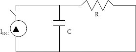
FIGURE 14.1 Simplified thermal circuit.

At time t = 0, the switch is closed and essentially all of the energy is absorbed by the capacitor. However, depending on the relative values of R and C, as time progresses, the capacitor is fully charged and essentially all of the current flows through the resistor. Thus, for cables subjected to large swings in loading for short periods of time, the thermal capacitance must be considered (see Section 14.4 of this chapter).

14.3.2 LOAD FACTOR

The ratio of average load to peak load is known as load factor. This is an important consideration since most loads on a utility system vary with the time of the day. The effect of this cyclic load on ampacity depends on the amount of thermal capacitance involved in the environment.

Cables in duct banks or directly buried in earth are surrounded by a substantial amount of thermal capacitance. The cable, surrounding ducts, concrete, and earth all take time to heat (and to cool). Thus, heat absorption takes place in those areas as the load increases and permits a higher ampacity than if the load had been continuous. Of course, cooling takes place during the dropping load portions of the load cycle.

For small cables in air or conduit in air, the thermal lag is small. The cables heat up relatively quickly, i.e., in 1 or 2 hours. For the usual load cycles, where the peak load exists for periods of 2 hours or more, load factor is not generally considered in determining the ampacity.

14.3.3 LOSS FACTOR

The loss factor may be calculated from the following formula when the daily load factor is known:

$L F = 0.3 (l f) + 0.7 {(l f)}^{2}$ $L F = 0.3 (l f) + 0.7 {(l f)}^{2}$

(14.2)

where LF = loss factor, and lf = daily load factor per unit.

Loss factor becomes significant at a specified distance from the center of the cable. This fictitious distance, D_x, derived by Neher and McGrath, is 8.3 inches (211 mm²). As the heat flows through the surrounding medium beyond this diameter, the effective rho becomes lower and hence the explanation of the role of the loss factor in that area.

14.3.4 CONDUCTOR LOSSES

When electric current flows through a material, there is a resistance to that flow. This is an inherent property of every material and the measure of this property is known as resistivity. The reciprocal of this property is conductivity. When selecting materials for use in an electrical conductor, it is desirable to use materials with as low a resistivity as is consistent with cost and ease of use.

Copper and aluminum are the ideal choices for use in power cables and are the dominant metals used throughout the world.

Regardless of the metal chosen for a cable, some resistance is encountered. It therefore becomes necessary to determine the electrical resistance of the conductor in order to calculate the ampacity of the cable. See Chapter 3 for details of the conductor loss calculation.

14.3.4.1 Direct Current Conductor Resistance

This subject has been introduced in Chapter 3. Some additional insight is presented here that applies directly to the determination of ampacity. The volume resistivity of annealed copper at 20°C is (Table 14.1):

$ρ_{20} = 0.017241 {ohm mm}^{2} / meter$ $ρ_{20} = 0.017241 {ohm mm}^{2} / meter$

(14.3)

In ohms-circular mil per foot units this becomes:

$ρ_{20} = 10.371 ohm-circular mil / foot$ $ρ_{20} = 10.371 ohm-circular mil / foot$

(14.4)

Conductivity of a conductor material is expressed as a relative quantity, i.e., as a percentage of a standard conductivity. The International Electrotechnical Commission (IEC) in 1913 adopted a resistivity value known as the International Annealed Copper Standard (IACS). The conductivity values for annealed copper were established as 100%.

TABLE 14.1
Direct Current Resistivity at 20°C

Metal	Volume Conductivity Percentage lACS	Volume Resistivity		Weight Resistivity Ohms-lb/mile²
Metal	Volume Conductivity Percentage lACS	Ohms-cmil/ft	Ohms-mm²/m	Weight Resistivity Ohms-lb/mile²
Soft copper	100.00	10.371	0.01724	875.2
Hard copper	96.16	10.785	0.01793	910.15
Copperweld	39.21	26.45	0.043971	2046.3
1350-H19	61.2	16.946	0.02817	434.81
5005-H19	53.5	19.385	0.03223	497.36
6201 T81	52.5	19.755	0.03284	506.85
Alumoweld	20.33	51.01	0.08401	3191.0
Steel	5.0	129.64	0.21551	9574.0

An aluminum conductor is typically 61.2% as conductive as an annealed copper conductor. Thus, a #1/0 AWG (53.5 mm²) solid aluminum conductor of 61.2% conductivity has a volume resistivity of 16.946 ohms—circular mil per foot and a cross-sectional area of 105,600 circular mils. Thus, the direct current (DC) resistance per 1,000 feet at 20°C is:

$R_{D C (20)} = 16, 946 \times 1, 000 / 105, 600$ $R_{D C (20)} = 16, 946 \times 1, 000 / 105, 600$

$R_{D C (20)} = 0.1605 ohms$ $R_{D C (20)} = 0.1605 ohms$

To adjust the tabulated values of conductor resistance to other temperatures that are commonly encountered, the following formula applies:

$R_{T 2} = R_{T 1} [1 + α (T_{2} - T_{1})]$ $R_{T 2} = R_{T 1} [1 + α (T_{2} - T_{1})]$

(14.5)

where

R_T2 = DC resistance of conductor at new temperature

R_T1 = DC resistance of conductor at “base” temperature

α = temperature coefficient of resistance

Temperature coefficients for various copper and aluminum conductors at several base temperatures are shown in Table 14.2.

14.3.4.2 Alternating Current Conductor Resistance

When the term “AC resistance of a conductor” is used, it means the DC resistance of that conductor plus an increment that reflects the increased apparent resistance in the conductor caused by the skin-effect inequality of current density. Skin effect results in a decrease of current density toward the center of a conductor. A longitudinal element of the conductor near the center is surrounded by more magnetic lines of force than is an element near the rim. Thus, the counter electromotive force (emf) is greater in the center of the element. The net driving emf at the center element is thus reduced with consequent reduction of current density.

Methods for calculating this increased resistance have been extensively treated in technical papers and bulletins, Reference [10] for instance.

TABLE 14.2
Temperature Coefficients for Conductor Metals

Metal	0°C	20°C	25°C	30°C
61.2% Al	0.00440	0.00404	0.00396	0.00389
100.0% Cu	0.00427	0.00393	0.00385	0.00378
98.0% Cu	0.00417	0.00385	0.00378	0.00371
96.0% Cu	0.00408	0.00377	0.00370	0.00364

14.3.4.3 Proximity Effect

The flux linking a conductor due to nearby current flow distorts the cross-sectional current distribution in the conductor in the same way as the flux from the current in the conductor itself. This is called proximity effect. Skin effect and proximity effect are seldom separable and the combined effects are not directly cumulative. If the distance between the conductors exceeds 10 times the diameter of a conductor, the extra I²R loss is negligible.

14.3.4.4 Hysteresis and Eddy Current Effects

Hysteresis and eddy current losses in conductors and adjacent metallic parts add to the effective alternating current (AC) resistance. To supply these losses, more power is required from the cable. They can be very significant in large ampacity conductors when the magnetic material is closely adjacent to the conductors. Currents greater than 200 amperes should be considered to be large for these effects.

14.3.5 CALCULATION OF DIELECTRIC LOSS

As has been seen in Chapter 4, dielectric losses may have an important effect on ampacity. For a single-conductor, shielded and for a multiconductor cable having shields over the individual conductors, the following formula applies:

$W_{d} = 2 π f C n E^{2} F_{p} \times 10^{- 6}$ $W_{d} = 2 π f C n E^{2} F_{p} \times 10^{- 6}$

(14.6)

and

$C = 7.354 ε / {Log}_{10} (D_{o} / D_{I})$ $C = 7.354 ε / {Log}_{10} (D_{o} / D_{I})$

(14.7)

where

f = operating frequency in hertz

n = number of shielded conductors in cable

C = capacitance of individual shielded conductors in micro-micro farads/ft

E = operating voltage to ground in kilovolts

F_p = power factor of insulation

ε = dielectric constant of the insulation

D_O = diameter over the insulation

D_I = diameter under the insulation

14.3.6 METALLIC SHIELD LOSSES

When current flows in a conductor, there is a magnetic field associated with that current flow. If the current varies in magnitude with time, such as with 60 hertz alternating current, the field expands and contracts with the current magnitude. In the event that a second conductor is within the magnetic field of the current carrying conductor, a voltage, which varies with the field, will be introduced in that conductor.

If that conductor is part of a circuit, the induced voltage will result in current flow. This situation occurs during operation of metallic shielded conductors. Current flow in the phase conductors induces a voltage in the metallic shields of all cables within the magnetic field. If the shields have two or more points that are grounded or otherwise complete a circuit, current will flow in the metallic shield conductor.

The current flowing in the metallic shields generates losses. The magnitude of the losses depends on the shield resistance and the current magnitude. This loss appears as heat. These losses not only represent an economic loss, but they also have a negative effect on ampacity and voltage drop. The heat generated in the shields must be dissipated along with the phase conductor losses and any dielectric loss. Recognizing that the amount of heat that can be dissipated is fixed for a given set of thermal conditions, the heat generated by the shields reduces the amount of heat that can be assigned to the phase conductor. This has the effect of reducing the permissible phase conductor current. In other words, shield losses reduce the allowable phase conductor ampacity.

In multiphase circuits, the voltage induced in any shield is the result of the vectoral addition and subtraction of all fluxes linking the shield. Since the net current in a balanced multiphase circuit is equal to zero when the shield wires are equidistant from all three phases, the net voltage is zero. This is usually not the case, so in the practical world there is some “net” flux that will induce a shield voltage/current flow. In a multiphase installation of shielded, single-conductor cables, as the spacing between conductors increases, the cancellation of flux from the other phases is reduced. The shield on each cable approaches the total flux linkage created by the phase conductor of that cable (Figure 14.2).

As the spacing, S, increases, the effect of phases B and C is reduced and the metallic shield losses in the A phase are almost entirely dependent on the A phase magnetic flux.

There are two general ways that the amount of shield losses can be minimized:

• Single point grounding (open circuit shield)

• Reduction of the quantity of metal in the shield

The open circuit shield presents other problems. The voltage continues to be induced and hence the voltage increases from zero at the point of grounding to a maximum at the open end that is remote from the ground. The magnitude of voltage is primarily dependent on the amount of current in the phase conductor. It follows that there are two current levels that must be considered: maximum normal current and maximum fault current in designing such a system. The amount of voltage that can be tolerated depends on safety concerns and jacket designs.

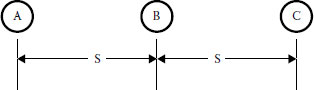
FIGURE 14.2 Effect of spacing.

Another approach is to reduce the amount of metal in the shield. Since the circuit is basically a one-to-one transformer, an increase in the resistance of the shield gives a reduction in the amount of current that will be generated in the shield. As an example, a 1,000 kcmil (507 mm²) aluminum conductor, three 15 kV cables with multiground neutrals that are installed in a flat configuration with 7.5 inch (190.5 mm²) spacing. A cable with one-third conductivity neutral will have four times as much current in the shields as a one-twelfth neutral cable. If the phase conductors are carrying a balanced 600 amperes, the outside, lagging phase cable will have 400 amperes in the shield. A similar cable configuration with one-twelfth neutral will have only 100 amperes. The total current is reduced from 1,000 amperes to 700 amperes. This translates to an increase of ampacity of roughly 25% for the reduced neutral cables.

In order to take shield losses into account when calculating ampacity, it is necessary to multiply all thermal resistances in the thermal circuit beyond the shield by one plus the ratio of the shield loss to the conductor loss. This incremental thermal resistance reflects the effect of the shield losses.

The shield loss calculations for cables in other configurations are rather complex, but very important. Halperin and Miller developed a method for closely approximating the losses and voltages for single-conductor cables in several common configurations.

14.4 TYPICAL THERMAL CIRCUITS

14.4.1 INTERNAL THERMAL CIRCUIT FOR A SHIELDED CABLE WITH JACKET

Thermal circuits will be shown in increasing complexity of the number of components. The symbols used throughout will be:

$\bar{R}$ $\bar{R}$ = thermal resistance (pronounced R bar) in thermal ohm-feet

Q = heat source in watts per foot

$\bar{C}$ $\bar{C}$ = thermal capacitance

The subscripts throughout are:

C = conductor

I = insulation

S = shield

J = jacket

D = duct

SD = distance between cable and duct

E = earth

14.4.2 SINGLE LAYER OF INSULATION, CONTINUOUS LOAD

The internal thermal circuit is shown in Figure 14.3 for a cable with continuous load. The conductor heat source passes through only one thermal resistance. This may be an insulation, a covering, or a combination as long as they have similar thermal resistances. Note that these circuits stop at the surface of the cable. The remainder of the thermal circuit will be added in examples that follow.

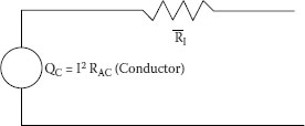
FIGURE 14.3 Continuous load flow.

Figure 14.3 shows a continuous load flowing through one layer of insulation. The heat does not travel beyond the surface of the cable in this example.

14.4.3 CABLE INTERNAL THERMAL CIRCUIT COVERED BY TWO DISSIMILAR MATERIALS, CONTINUOUS LOAD

In this example, the continuous load flows through two dissimilar materials, but the heat still stays at the surface of the last layer of insulation (Figure 14.4).

14.4.4 CABLE THERMAL CIRCUIT FOR PRIMARY CABLE WITH METALLIC SHIELD AND JACKET, CONTINUOUS LOAD

This thermal diagram (Figure 14.5) shows a primary cable with its several heat sources and thermal resistances still with a constant load where p and (1−p) divide the thermal resistance to reflect Q_i.

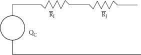
FIGURE 14.4 Load flow through two materials.

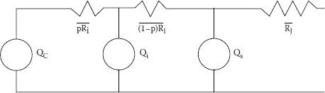
FIGURE 14.5 Shielded cable with several heat sources.

14.4.5 SAME CABLE AS EXAMPLE 3, BUT WITH CYCLIC LOAD

Figure 14.6 shows the same cable as in Figure 14.5, but the cyclic load is accounted for with the capacitors that are parallel to the three heat sources.

14.4.6 EXTERNAL THERMAL CIRCUIT, CABLE IN DUCT, CONTINUOUS LOAD

Figure 14.7 shows the resistances that are external to the cable.

14.4.7 EXTERNAL THERMAL CIRCUIT, CABLE IN DUCT, TIME VARYING LOAD, EXTERNAL HEAT SOURCE

See Figure 14.8, where H_X = external heat Source.

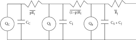
FIGURE 14.6 Cyclic load has been added.

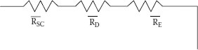
FIGURE 14.7 External circuit.

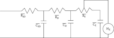
FIGURE 14.8 External heat source added.

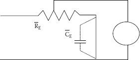
FIGURE 14.9 External thermal circuit.

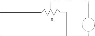
FIGURE 14.10 Cable in air.

14.4.8 EXTERNAL THERMAL CIRCUIT, CABLE BURIED IN EARTH, LOAD MAY BE CYCLIC, EXTERNAL HEAT SOURCE MAY BE PRESENT

The depiction of possible cyclic load and external heat source is shown in Figure 14.9 by dotted lines.

14.4.9 EXTERNAL THERMAL CIRCUIT, CABLE IN AIR, POSSIBLE EXTERNAL HEAT SOURCE

The external thermal circuit is shown in Figure 14.10 with the possible external heat source shown by dotted lines.

14.5 SAMPLE AMPACITY CALCULATION

14.5.1 GENERAL

Methods to calculate the ampacity of operating cables continue to be a popular subject for technical papers. Fortunately, the portion of the work that had been done by slide-rule and copious quantities of notepaper has been replaced with computers. Manipulations were handled by assuming intermediate values of the various parameters prior to the advent of the computer. The hand calculations were laborious, but the user did get a feel for the concept. The availability of tables and computer programs could lead to quick, but possibly incorrect, answers. The Neher–McGrath paper [10] is the best reference to use before a hand calculation is attempted. As a matter of fact, you should read that paper even if you have decided to use any available tables or programs!

The following simple example of a calculation is presented with the intent of giving insight into the process.

The general equation that has been previously given in Equation 14.1.

Another form of this equation recognizes the other possible heat sources that have been indicated in the thermal circuit diagrams. Equation 14.1 expands to:

$I = \sqrt{\frac{T_{C} - (T_{A} + Δ T_{d})}{R_{A C} (\bar{R_{i}} + \bar{R_{T H}})}}$ $I = \sqrt{\frac{T_{C} - (T_{A} + Δ T_{d})}{R_{A C} (\bar{R_{i}} + \bar{R_{T H}})}}$

(14.8)

where

ΔT_d = temperature rise due to dielectric loss in °C

$\bar{R_{i}}$ $\bar{R_{i}}$ = to account for thermal resistance of insulation and/or coverings between the conductor and the first heat source beyond the insulation.

$\bar{R_{T H}}$ $\bar{R_{T H}}$ = is the thermal resistance to ambient adjusted to account for additional heat sources such as shield loss, armor loss, steam lines, etc.

14.6 AMPACITY TABLES AND COMPUTER PROGRAMS

14.6.1 TABLES

The IEEE Standard Power Cable Ampacity Tables, [11,12], IEEE Standard 835-1994, is a book (or electronic version) that contains over 3,000 tables in 3,086 pages. Voltages range from 5 kV to 138 kV. Although there are situations that are not covered by these tables, this is an excellent beginning point for anyone interested in cable ampacities.

ICEA P-54-440, Ampacities of Cables in Open Top Trays covers ampacities in trays that is not covered in IEEE Standard 835.

The early ampacity tables AIEE S-135, Volumes 1 & 2, IPCEA Pub. P-46-426, 1962 continue to be used for appropriate situations.

It is important to point out that situations in the US falling under the jurisdiction of the National Electric Code are covered by the ampacity tables found in NFPA 70, National Electrical Code. Similar codes may be expected to exist in every country outside the US and the reader is advised to consult them as appropriate.

Manufacturers have also published catalogs that cover the more common situations [13,14].

14.6.2 COMPUTER PROGRAMS

Most of the large cable manufacturers and architect/engineering firms have their own computer programs for ampacity determination. This is an excellent source of information when you are engineering a new cable system. These programs generally are not for sale.

There are commercially available programs throughout North America. These are especially useful when you need to determine the precise ampacity of a cable, for instance, in a duct bank with other cables that are not fully loaded. The general cost of one of these programs is about $5,000 in US dollars.

14.7 “AMPACITIES” UNDER SHORT CIRCUIT CONDITIONS

Short circuit conditions commonly involve large inrushes of current. The heating associated with these can be extremely destructive and hazardous. Calculations to determine the capability of cables to withstand these currents (and durations) are generally handled by other calculation methods and assumptions.

In North America, some common methods are found in:

ICEA P-32-382 “Short Circuit Characteristics of Insulated Cables” latest edition

ICEA P-45-482 “Short Circuit Performance of Metallic Shields and Sheaths of Insulated Cable” latest edition

EPRI EL-3014, Project 1286-2, final report 4/83, “Optimization of Design of Metallic Shield–Concentric Conductors of Extruded Dielectric Cables Under Fault Conditions”

Similar methods are published in IEC 60949-9, “Calculations of Thermally Permissible Short Currents Taking Into Account Non-Adiabatic Heating Effects” and other national standards.

14.8 RELATIONSHIPS BETWEEN AMPACITY AND VOLTAGE DROP CALCULATIONS

Factors that impact ampacity calculations also impact voltage drop calculations. The AC and DC resistances of conductors increase with increasing temperature, thereby increasing voltage drop. Similarly, shield, sheath, and pipe losses have the effect of increasing the apparent conductor resistance and impacting inductive reactance. An excellent reference that discusses these relationships is reference [9].

REFERENCES

1. Power Cable Ampacities, 1962, AIEE Pub. No. S-135-1 and IPCEA Pub. No. P-46-426.

2. Kennelly, A. E., 1893, “On the Carrying Capacity of Electrical Cables…”, Minutes, Ninth Annual Meeting, Association of Edison Illuminating Companies, New York, NY.

3. Neher, J. H., 31 January–4 February 1949, “The Temperature Rise of Buried Cables and Pipes,” AIEE Paper No. 49-2, Winter General Meeting, New York, NY.

4. Balaska, T. A., McKean, A. L. and Merrell, E. J., 19–24 June 1960, “Long Time Heat Runs on Underground Cables in a Sand Hill,” AIEE Paper No. 60-809, Summer General Meeting.

5. Schmill, J. V., 30 January–4 February 1966, “Variable Soil Thermal Resistivity – Steady State Analysis,” IEEE Paper. No. 31 TP 66-14, Winter Power Meeting, New York, NY.

6. Insulated Conductors Committee Minutes, Appendices F-3, F-4, F-5, F-6, F-7, and F-8, November 1984.

7. IEEE Guide for Soil Thermal Resistivity Measurements, IEEE Std. 442-1979.

8. Black, W. Z. and Martin, M. A. Jr., 1–8 February 1981, “Practical Aspects of Applying Thermal Stability Measurements to the Rating of Underground Power Cables,” IEEE Paper No. 81 WM 050-4, Atlanta, GA.

9. Simmons, D. M., May–November 1932, “Calculation of the Electrical Problems of Underground Cables,” The Electrical Journal, East Pittsburgh, PA.

10. Neher, J. H. and McGrath, M. H., October 1957, “The Calculation of the Temperature Rise and Load Capability of Cable Systems,” AIEE Transactions, Vol. 76, Pt. III, pp. 752–772.

11. IEEE Standard Power Cable Ampacity Tables, IEEE Std. 835-1994 (hard copy version).

12. IEEE Standard Power Cable Ampacity Tables, IEEE Std. 835-1994 (electronic version).

13. Engineering Data for Copper and Aluminum Conductor Electrical Cables, 1990, EHB-90, The Okonite Company.

14. Power Cable Manual, 1997, Second Edition, The Southwire Company.

..................Content has been hidden....................

You can't read the all page of ebook, please click here login for view all page.

Table of Contents for Chapter 14 Ampacity of Cables

Create new playlist

Sign In

Sign Up

Table of Contents for
Chapter 14 Ampacity of Cables