2. Conversion and Reactor Sizing
Be more concerned with your character than with your reputation, because character is what you really are while reputation is merely what others think you are.
—John Wooden, head coach, UCLA Bruins
2.1 Definition of Conversion
In defining conversion, we choose one of the reactants as the basis of calculation and then relate the other species involved in the reaction to this basis. In virtually all instances we must choose the limiting reactant as the basis of calculation. We develop the stoichiometric relationships and design equations by considering the general reaction
The uppercase letters represent chemical species, and the lowercase letters represent stoichiometric coefficients. We shall choose species A as our limiting reactant and, thus, our basis of calculation. The limiting reactant is the reactant that will be completely consumed first after the reactants have been mixed. Next, we divide the reaction expression through by the stoichiometric coefficient of species A, in order to arrange the reaction expression in the form
to put every quantity on a “per mole of A” basis, our limiting reactant.
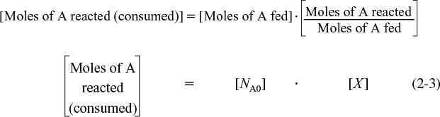
Now we ask such questions as “How can we quantify how far a reaction [e.g., Equation (2-2)] proceeds to the right?” or “How many moles of C are formed for every mole of A consumed?” A convenient way to answer these questions is to define a parameter called conversion. The conversion XA is the number of moles of A that have reacted per mole of A fed to the system:
Definition of X
Because we are defining conversion with respect to our basis of calculation [A in Equation (2-2)], we eliminate the subscript A for the sake of brevity and let .X ≡ XA. For irreversible reactions, the maximum conversion is 1.0, i.e., complete conversion. For reversible reactions, the maximum conversion is the equilibrium conversion Xe (i.e., Xmax = Xe). We will take a closer look at equilibrium conversion in Chapter 4.
2.2 Batch Reactor Design Equations
In most batch reactors, the longer a reactant stays in the reactor, the more the reactant is converted to product until either equilibrium is reached or the reactant is exhausted. Consequently, in batch systems the conversion X is a function of the time the reactants spend in the reactor. If NA0 is the number of moles of A initially present in the reactor (i.e., t = 0), then the total number of moles of A that have reacted (i.e., have been consumed) after a time t is [NA0X]
Now, the number of moles of A that remain in the reactor after a time t, NA, can be expressed in terms of NA0 and X:
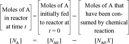
The number of moles of A in the reactor after a conversion X has been achieved is
Moles of A in the reactor at a time t
When no spatial variations in reaction rate exist, the mole balance on species A for a batch system is given by the following equation [cf. Equation (1-5)]:
This equation is valid whether or not the reactor volume is constant. In the general reaction, Equation (2-2), reactant A is disappearing; therefore, we multiply both sides of Equation (2-5) by –1 to obtain the mole balance for the batch reactor in the form
The rate of disappearance of A, –rA, in this reaction might be given by a rate law similar to Equation (1-2), such as –rA = kCACB.
For batch reactors, we are interested in determining how long to leave the reactants in the reactor to achieve a certain conversion X. To determine this length of time, we write the mole balance, Equation (2-5), in terms of conversion by differentiating Equation (2-4) with respect to time, remembering that NA0 is the number of moles of A initially present in the reactor and is therefore a constant with respect to time.
Combining the above with Equation (2-5) yields
For a batch reactor, the design equation in differential form is
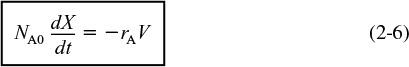
Batch reactor (BR) design equation
We call Equation (2-6) the differential form of the design equation for a batch reactor because we have written the mole balance in terms of conversion. The differential forms of the batch reactor mole balances, Equations (2-5) and (2-6), are often used in the interpretation of reaction rate data (Chapter 7) and for reactors with heat effects (Chapters 11-13), respectively. Batch reactors are frequently used in industry for both gas-phase and liquid-phase reactions. The laboratory bomb calorimeter reactor is widely used for obtaining reaction rate data. Liquid-phase reactions are frequently carried out in batch reactors when small-scale production is desired or operating difficulties rule out the use of continuous-flow systems.
To determine the time to achieve a specified conversion X, we first separate the variables in Equation (2-6) as follows:
Batch time t to achieve a conversion X
This equation is now integrated with the limits that the reaction begins at time equals zero where there is no conversion initially (when t = 0, X = 0) and ends at time t when a conversion X is achieved (i.e., when t = t, then X = X). Carrying out the integration, we obtain the time t necessary to achieve a conversion X in a batch reactor
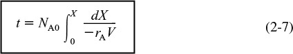
Batch Design Equation
The longer the reactants are left in the reactor, the greater the conversion will be. Equation (2-6) is the differential form of the design equation, and Equation (2-7) is the integral form of the design equation for a batch reactor.
2.3 Design Equations for Flow Reactors
For a batch reactor, we saw that conversion increases with time spent in the reactor. For continuous-flow systems, this time usually increases with increasing reactor volume, e.g., the bigger/longer the reactor, the more time it will take the reactants to flow completely through the reactor and thus, the more time to react. Consequently, the conversion X is a function of reactor volume V. If FA0 is the molar flow rate of species A fed to a system operated at steady state, the molar rate at which species A is reacting within the entire system will be FA0X.

The molar feed rate of A to the system minus the rate of reaction of A within the system equals the molar flow rate of A leaving the system FA. The preceding sentence can be expressed mathematically as
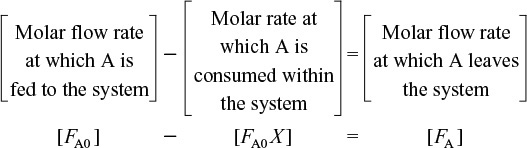
Rearranging gives
The entering molar flow rate of species A, FA0 (mol/s), is just the product of the entering concentration, CA0 (mol/dm3), and the entering volumetric flow rate, υ0 (dm3/s).
Liquid phase
For liquid systems, the volumetric flow rate, υ, is constant and equal to, and CA0 is commonly given in terms of molarity, for example, CA0 = 2 mol/dm3.
For gas systems, CA0 can be calculated from the entering mole fraction, yA0, the temperature, T0, and pressure, P0, using the ideal gas law or some other gas law. For an ideal gas (see Appendix B):
Gas phase
Now that we have a relationship [Equation (2-8)] between the molar flow rate and conversion, it is possible to express the design equations (i.e., mole balances) in terms of conversion for the flow reactors examined in Chapter 1.
2.3.1 CSTR (Also Known as a Backmix Reactor or a Vat)
Recall that the CSTR is modeled as being well mixed such that there are no spatial variations in the reactor. For the general reaction
the CSTR mole balance Equation (1-7) can be arranged to
We now substitute for FA in terms of FA0 and X
and then substitute Equation (2-12) into (2-11)

Perfect mixing
Simplifying, we see that the CSTR volume necessary to achieve a specified conversion X is

Because the reactor is perfectly mixed, the exit composition from the reactor is identical to the composition inside the reactor, and, therefore, the rate of reaction, –rA is evaluated at the exit conditions.
Evaluate –rA at the CSTR exit conditions!!
2.3.2 Tubular Flow Reactor (PFR)
We model the tubular reactor as having the fluid flowing in plug flow—i.e., no radial gradients in concentration, temperature, or reaction rate.1 As the reactants enter and flow axially down the reactor, they are consumed and the conversion increases along the length of the reactor. To develop the PFR design equation, we first multiply both sides of the tubular reactor design equation (1-12) by –1. We then express the mole balance equation for species A in the reaction as
1 This constraint can be removed when we extend our analysis to nonideal (industrial) reactors in Chapters 16 through 18.
For a flow system, FA has previously been given in terms of the entering molar flow rate FA0 and the conversion X
Differentiating
dFA = –FA0dX
and substituting into (2-14) gives the differential form of the design equation for a plug-flow reactor (PFR)

We now separate the variables and integrate with the limits V = 0 when X = 0 to obtain the plug-flow reactor volume necessary to achieve a specified conversion X

To carry out the integrations in the batch and plug-flow reactor design equations (2-7) and (2-16), as well as to evaluate the CSTR design equation (2-13), we need to know how the reaction rate –rA varies with the concentration (hence conversion) of the reacting species. This relationship between reaction rate and concentration is developed in Chapter 3.
2.3.3 Packed-Bed Reactor (PBR)
Packed-bed reactors are tubular reactors filled with catalyst particles. In PBRs it is the weight of catalyst W that is important, rather than the reactor volume. The derivation of the differential and integral forms of the design equations for packed-bed reactors are analogous to those for a PFR [cf. Equations (2-15) and (2-16)]. That is, substituting Equation (2-12) for FA in Equation (1-15) gives

PBR design equation
The differential form of the design equation [i.e., Equation (2-17)] must be used when analyzing reactors that have a pressure drop along the length of the reactor. We discuss pressure drop in packed-bed reactors in Chapter 5.
In the absence of pressure drop, i.e., ΔP = 0, we can integrate (2-17) with limits X = 0 at W = 0, and when W = W then X = X to obtain


Equation (2-18) can be used to determine the catalyst weight W (i.e., mass) necessary to achieve a conversion X when the total pressure remains constant.
2.4 Sizing Continuous-Flow Reactors
In this section, we are going to show how we can size CSTRs and PFRs (i.e., determine their reactor volumes) from knowledge of the rate of reaction, –rA, as a function of conversion, X [i.e., –rA = f(X)]. The rate of disappearance of A, –rA, is almost always a function of the concentrations of the various species present (see Chapter 3). When only one reaction is occurring, each of the concentrations can be expressed as a function of the conversion X (see Chapter 4); consequently, –rA can be expressed as a function of X.
A particularly simple functional dependence, yet one that occurs often, is the first-order dependence
–rA = kCA = kCA0(1 – X)
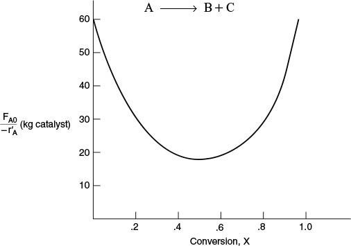
Here, k is the specific reaction rate and is a function only of temperature, and CA0 is the entering concentration of A. We note in Equations (2-13) and (2-16) that the reactor volume is a function of the reciprocal of –rA. For this first-order dependence, a plot of the reciprocal rate of reaction (1/–rA) as a function of conversion yields a curve similar to the one shown in Figure 2-1, where

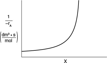
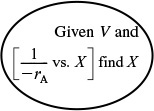
We can use Figure 2-1 to size CSTRs and PFRs for different entering flow rates. By sizing we mean either determine the reactor volume for a specified conversion or determine the conversion for a specified reactor volume. Before sizing flow reactors, let’s consider some insights. If a reaction is carried out isothermally, the rate is usually greatest at the start of the reaction when the concentration of reactant is greatest (i.e., when there is negligible conversion [X ≅ 0]). Hence, the reciprocal rate (1/–rA) will be small. Near the end of the reaction, when the reactant has been mostly used up and thus the concentration of A is small (i.e., the conversion is large), the reaction rate will be small. Consequently, the reciprocal rate (1/–rA) is large.
For all irreversible reactions of greater than zero order (see Chapter 3 for zero-order reactions), as we approach complete conversion where all the limiting reactant is used up, i.e., X = 1, the reciprocal rate approaches infinity as does the reactor volume, i.e.
As X → 1, –rA → 0, thus, ![]() and therefore V → ∞
and therefore V → ∞
A → B + C
“To infinity and beyond” –Buzz Lightyear
Consequently, we see that an infinite reactor volume is necessary to reach complete conversion, X = 1.0.
For reversible reactions (e.g., A ![]() B), the maximum conversion is the equilibrium conversion Xe. At equilibrium, the reaction rate is zero (rA ≡ 0). Therefore,
B), the maximum conversion is the equilibrium conversion Xe. At equilibrium, the reaction rate is zero (rA ≡ 0). Therefore,
as X → Xe, –rA → 0, thus, ![]() and therefore V → ∞
and therefore V → ∞
A ![]() B + C
B + C
and we see that an infinite reactor volume would also be necessary to obtain the exact equilibrium conversion, X = Xe. We will discuss Xe further in Chapter 4.
Examples of Reactor Design and Staging Given –rA = f(X)
To illustrate the design of continuous-flow reactors (i.e., CSTRs and PFRs), we consider the isothermal gas-phase isomerization
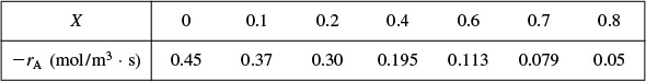
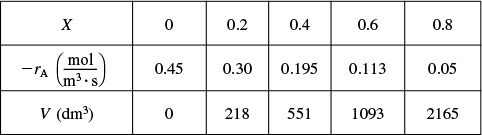
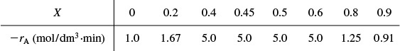
We are going to the laboratory to determine the rate of chemical reaction as a function of the conversion of reactant A. The laboratory measurements given in Table 2-1 show the chemical reaction rate as a function of conversion. The temperature was 500 K (440°F), the total pressure was 830 kPa (8.2 atm), and the initial charge to the reactor was pure A. The entering molar flow of A rate is FA0 = 0.4 mol/s.
† Proprietary coded data courtesy of Jofostan Central Research Laboratory, Çölow, Jofostan, and published in Jofostan Journal of Chemical Engineering Research, Volume 21, page 73 (1993).
TABLE 2-1 RAW DATA†
If we know –rA as a function of X, we can size any isothermal reaction system.
Recalling the CSTR and PFR design equations, (2-13) and (2-16), we see that the reactor volume varies directly with the molar flow rate FA0 and with the reciprocal of –rA, ![]() , e.g.,
, e.g., ![]() . Consequently, to size reactors, we first convert the raw data in Table 2-1, which gives –rA as a function of X first to
. Consequently, to size reactors, we first convert the raw data in Table 2-1, which gives –rA as a function of X first to ![]() as a function of X. Next, we multiply by the entering molar flow rate, FA0, to obtain
as a function of X. Next, we multiply by the entering molar flow rate, FA0, to obtain ![]() as a function of X as shown in Table 2-2 of the processed data for FA0 = 0.4 mol/s.
as a function of X as shown in Table 2-2 of the processed data for FA0 = 0.4 mol/s.

We shall use the data in this table for the next five Example Problems.
To size reactors for different entering molar flow rates, FA0, we would use rows 1 and 3 in Table 2-2 to construct the following figure:
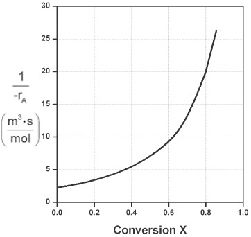
However, for a given FA0, rather than use Figure 2-2A to size reactors, it is often more advantageous to plot ![]() as a function of X, which is called a Levenspiel plot. We are now going to carry out a number of examples where we have specified the flow rate FA0 at 0.4 mol A/s.
as a function of X, which is called a Levenspiel plot. We are now going to carry out a number of examples where we have specified the flow rate FA0 at 0.4 mol A/s.
Plotting ![]() as a function of X using the data in Table 2-2 we obtain the plot shown in Figure 2-2B.
as a function of X using the data in Table 2-2 we obtain the plot shown in Figure 2-2B.
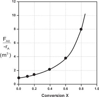
Levenspiel plot
We are now going to use the Levenspiel plot of the processed data (Figure 2-2B) to size a CSTR and a PFR.
The reaction described by the data in Table 2-2
A → B
is to be carried out in a CSTR. Species A enters the reactor at a molar flow rate of ![]() , which is the flow rate used to construct Figure 2-2B.
, which is the flow rate used to construct Figure 2-2B.
(a) Using the data in either Table 2-2 or Figure 2-2B, calculate the volume necessary to achieve 80% conversion in a CSTR.
(b) Shade the area in Figure 2-2B that would give the CSTR volume necessary to achieve 80% conversion.
Solutions
(a) Equation (2-13) gives the volume of a CSTR as a function of FA0, X, and –rA

In a CSTR, the composition, temperature, and conversion of the effluent stream are identical to that of the fluid within the reactor, because perfect mixing is assumed. Therefore, we need to find the value of –rA (or reciprocal thereof) at X = 0.8. From either Table 2-2 or Figure 2-2A, we see that when X = 0.8, then
Substitution into Equation (2-13) for an entering molar flow rate, FA0, of 0.4 mol A/s and X = 0.8 gives

(b) Shade the area in Figure 2-2B that yields the CSTR volume. Rearranging Equation (2-13) gives
In Figure E2-1.1, the volume is equal to the area of a rectangle with a height (FA0/–rA = 8 m3) and a base (X = 0.8). This rectangle is shaded in the figure.
V = Levenspiel rectangle area = height × width
V = [8 m3][0.8] = 6.4 m3 = 6400 dm3 = 6400 L
Representative Industrial CSTR Dimensions
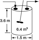
The CSTR volume necessary to achieve 80% conversion is 6.4 m3 when operated at 500 K, 830 kPa (8.2 atm), and with an entering molar flow rate of A of 0.4 mol/s. This volume corresponds to a reactor about 1.5 m in diameter and 3.6 m high. It’s a large CSTR, but this is a gas-phase reaction, and CSTRs are normally not used for gas-phase reactions. CSTRs are used primarily for liquid-phase reactions.

Plots of (FA0/–rA) vs. X are sometimes referred to as Levenspiel plots (after Octave Levenspiel).
Analysis: Given the conversion, the rate of reaction as a function of conversion along with the molar flow of the species A, we saw how to calculate the volume of a CSTR. From the data and information given, we calculated the volume to be 6.4 m3 for 80% conversion. We showed how to carry out this calculation using the design equation (2-13) and also using a Levenspiel plot.
The reaction described by the data in Tables 2-1 and 2-2 is to be carried out in a PFR. The entering molar flow rate of A is again 0.4 mol/s.
(a) First, use one of the integration formulas given in Appendix A.4 to determine the PFR reactor volume necessary to achieve 80% conversion.
(b) Next, shade the area in Figure 2-2B that would give the PFR volume necessary to achieve 80% conversion.
(c) Finally, make a qualitative sketch of the conversion, X, and the rate of reaction, –rA, down the length (volume) of the reactor.
Solution
We start by repeating rows 1 and 4 of Table 2-2 to produce the results shown in Table 2-3.
(a) Numerically evaluate PFR volume. For the PFR, the differential form of the mole balance is
Rearranging and integrating gives

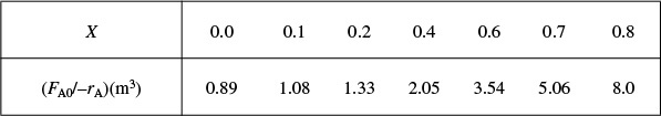
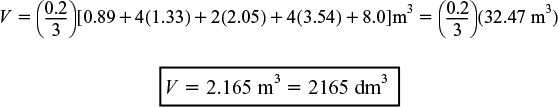
We shall use the five-point quadrature formula [Equation (A-23)] given in Appendix A.4 to numerically evaluate Equation (2-16). The five-point formula with a final conversion of 0.8 gives four equal segments between X = 0 and X = 0.8, with a segment length of ![]() . The function inside the integral is evaluated at X = 0, X = 0.2, X = 0.4, X = 0.6, and X = 0.8.
. The function inside the integral is evaluated at X = 0, X = 0.2, X = 0.4, X = 0.6, and X = 0.8.

Using values of [FA0/(–rA)] corresponding to the different conversions in Table 2-3 yields
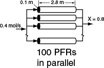
The PFR reactor volume necessary to achieve 80% conversion is 2165 dm3. This volume could result from a bank of 100 PFRs that are each 0.1 m in diameter with a length of 2.8 m (e.g., see margin figure or Figures 1-8(a) and (b)).
(b) The PFR volume, i.e., the integral in Equation (2-16), can also be evaluated from the area under the curve of a plot of (FA0/–rA) versus X.
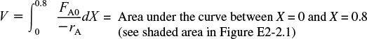
PFR
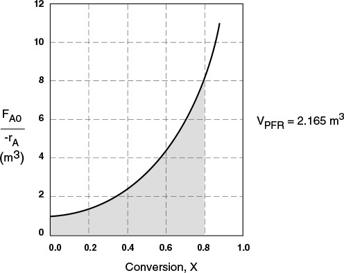
The area under the curve will give the tubular reactor volume necessary to achieve the specified conversion of A. For 80% conversion, the shaded area is roughly equal to 2165 dm3 (2.165 m3).
(c) Sketch the profiles of –rA and X down the length of the reactor.
We know that as we proceed down the reactor, the conversion increases as more and more reactant is converted to product. Consequently, as the reactant is consumed, the concentration of reactant decreases, as does the rate of disappearance of A for isothermal reactions.
(i) For X = 0.2, we calculate the corresponding reactor volume using Simpson’s rule [given in Appendix A.4 as Equation (A-21)] with increment ΔX = 0.1 and the data in rows 1 and 4 in Table 2-2.
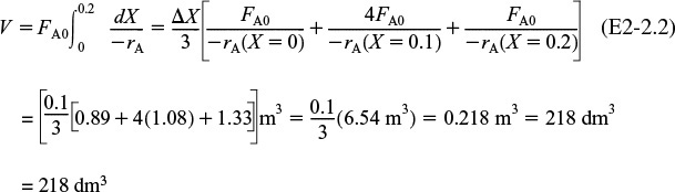
This volume (218 dm3) is the volume at which X = 0.2. From Table 2-3, we see the corresponding rate of reaction at X = 0.2 is ![]() .
.
Therefore at X = 0.2, then ![]() and V = 218 dm3.
and V = 218 dm3.
(ii) For X = 0.4, we can again use Table 2-3 and Simpson’s rule with ΔX = 0.2 to find the reactor volume necessary for a conversion of 40%.
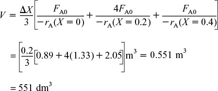
From Table 2-3 we see that at X = 0.4, ![]() and V= 551 dm3.
and V= 551 dm3.
We can continue in this manner to arrive at Table E2-2.1.
The data in Table E2-2.1 are plotted in Figures E2-2.2(a) and (b).
For isothermal reactions, the conversion increases and the rate decreases as we move down the PFR.


Analysis: One observes that the reaction rate, –rA, decreases as we move down the reactor while the conversion increases. These plots are typical for reactors operated isotherm ally.
Example 2–3 Comparing CSTR and PFR Sizes
Compare the volumes of a CSTR and a PFR required for the same conversion using the data in Figure 2-2B. Which reactor would require the smaller volume to achieve a conversion of 80%: a CSTR or a PFR? The entering molar flow rate and the feed conditions are the same in both cases.
Solution
We will again use the data in Table 2-3.
The CSTR volume was 6.4 m3 and the PFR volume was 2.165 m3. When we combine Figures E2-1.1 and E2-2.1 on the same graph, Figure 2-3.1(a), we see that the crosshatched area above the curve is the difference in the CSTR and PFR reactor volumes.
For isothermal reactions greater than zero order (see Chapter 3), the CSTR volume will always be greater than the PFR volume for the same conversion and reaction conditions (temperature, flow rate, etc.).
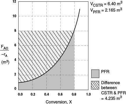

Figure E2-3.1(b) –rA as a function of X obtained from Table 2-2.1.
Analysis: We see that the reason the isothermal CSTR volume is usually greater than the PFR volume is that the CSTR is always operating at the lowest reaction rate (e.g., –rA = 0.05 mol/m3 · s in Figure E2-3.1(b)). The PFR, on the other hand, starts at a high rate at the entrance and gradually decreases to the exit rate, thereby requiring less volume because the volume is inversely proportional to the rate. However, there are exceptions such as autocatalytic reactions, product-inhibited reactions, and nonisothermal exothermic reactions; these trends will not always be the case, as we will see in Chapters 9 and 11.
2.5 Reactors in Series
Many times, reactors are connected in series so that the exit stream of one reactor is the feed stream for another reactor. When this arrangement is used, it is often possible to speed calculations by defining conversion in terms of location at a point downstream rather than with respect to any single reactor. That is, the conversion X is the total number of moles of A that have reacted up to that point per mole of A fed to the first reactor.
Only valid for NO side streams!!
For reactors in series


However, this definition can only be used when the feed stream only enters the first reactor in the series and there are no side streams either fed or withdrawn. The molar flow rate of A at point i is equal to the moles of A fed to the first reactor, minus all the moles of A reacted up to point i.
FAi = FA0 – FA0Xi
For the reactors shown in Figure 2-3, X1 at point i = 1 is the conversion achieved in the PFR, X2 at point i = 2 is the total conversion achieved at this point in the PFR and the CSTR, and X3 is the total conversion achieved by all three reactors.

To demonstrate these ideas, let us consider three different schemes of reactors in series: two CSTRs, two PFRs, and then a combination of PFRs and CSTRs in series. To size these reactors, we shall use laboratory data that give the reaction rate at different conversions.
2.5.1 CSTRs in Series
The first scheme to be considered is the two CSTRs in series shown in Figure 2-4.

For the first reactor, the rate of disappearance of A is –rA1 at conversion X1.
A mole balance on reactor 1 gives

The molar flow rate of A at point 1 is
Combining Equations (2-19) and (2-20), or rearranging
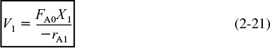
Reactor 1
In the second reactor, the rate of disappearance of A, –rA2, is evaluated at the conversion of the exit stream of reactor 2, X2. A steady-state mole balance on the second reactor is

The molar flow rate of A at point 2 is
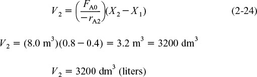
Combining and rearranging

Reactor 2
For the second CSTR, recall that –rA2 is evaluated at X2 and then use (X2–X1) to calculate V2.
In the examples that follow, we shall again use the molar flow rate of A used in Example 2-1 (i.e., FA0 = 0.4 mol A/s) and the reaction conditions given in Table 2-3.
Example 2–4 Comparing Volumes for CSTRs in Series
For the two CSTRs in series, 40% conversion is achieved in the first reactor. What is the volume of each of the two reactors necessary to achieve 80% overall conversion of the entering species A? (See Table 2-3.)
For Reactor 1, we observe from either Table 2-3 or Figure 2-2B that when X = 0.4, then
Then, using Equation (2-13)
For Reactor 2, when X2 = 0.8, then ![]() using Equation (2-24)
using Equation (2-24)
To achieve the same overall conversion, the total volume for two CSTRs in series is less than that required for one CSTR.

The shaded areas in Figure E2-4.1 can also be used to determine volumes of CSTR 1 and CSTR 2.
Note again that for CSTRs in series, the rate –rA1 is evaluated at a conversion of 0.4 and rate –rA2 is evaluated at a conversion of 0.8. The total volume for these two reactors in series is
V = V1 + V2 = 0.82 m3 + 3.2 m3 = 4.02 m3 = 4020 dm3
By comparison, the volume necessary to achieve 80% conversion in one CSTR is
We need only –rA = f(X) and FA0 to size reactors.
Notice in Example 2-5 that the sum of the two CSTR reactor volumes (4.02 m3) in series is less than the volume of one CSTR (6.4 m3) to achieve the same overall conversion.
Analysis: When we have reactors in series, we can speed our analysis and calculations by defining an overall conversion at a point in the series, rather than the conversion of each individual reactor. In this example, we saw that 40% was achieved at point 1, the exit to the first reactor, and that a total of 80% conversion was achieved by the time we exit the second reactor.
Approximating a PFR by a Large Number of CSTRs in Series
Consider approximating a PFR with a number of small, equal-volume CSTRs of Vi in series (Figure 2-5). We want to compare the total volume of all the CSTRs with the volume of one plug-flow reactor for the same conversion, say 80%.
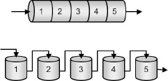
The fact that we can model a PFR with a large number of CSTRs is an important result.
From Figure 2-6, we note a very important observation! The total volume to achieve 80% conversion for five CSTRs of equal volume in series is “roughly” the same as the volume of a PFR. As we make the volume of each CSTR smaller and increase the number of CSTRs, the total volume of the CSTRs in series and the volume of the PFR will become identical. That is, we can model a PFR with a large number of CSTRs in series. This concept of using many CSTRs in series to model a PFR will be used later in a number of situations, such as modeling catalyst decay in packed-bed reactors or transient heat effects in PFRs.
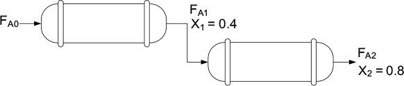
2.5.2 PFRs in Series
We saw that two CSTRs in series gave a smaller total volume than a single CSTR to achieve the same conversion. This case does not hold true for the two plug-flow reactors connected in series shown in Figure 2-7.
PFRS in series
We can see from Figure 2-8 and from the following equation
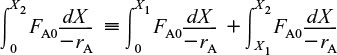
that it is immaterial whether you place two plug-flow reactors in series or have one continuous plug-flow reactor; the total reactor volume required to achieve the same conversion is identical!

The overall conversion of two PFRs in series is the same as one PFR with the same total volume.
2.5.3 Combinations of CSTRs and PFRs in Series
The final sequences we shall consider are combinations of CSTRs and PFRs in series. An industrial example of reactors in series is shown in the photo in Figure 2-9. This sequence is used to dimerize propylene (A) into olefins (B), e.g.,
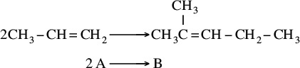
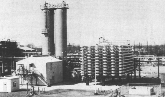
Figure 2-9 Dimersol G (an organometallic catalyst) unit (two CSTRs and one tubular reactor in series) to dimerize propylene into isohexanes. Institut Français du Pétrole process. Photo courtesy of Editions Technip (Institut Français du Pétrole).
Not sure if the size of these CSTRs is in the Guiness Book of World Records
A schematic of the industrial reactor system in Figure 2-9 is shown in Figure 2-10.

For the sake of illustration, let’s assume that the reaction carried out in the reactors in Figure 2-10 follows the same ![]() vs. X curve given by Table 2-3.
vs. X curve given by Table 2-3.
The volumes of the first two CSTRs in series (see Example 2-5) are:
In this series arrangement, –rA2 is evaluated at X2 for the second CSTR.
Starting with the differential form of the PFR design equation
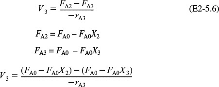
rearranging and integrating between limits, when V = 0, then X = X2, and when V = V3, then X = X3 we obtain

The corresponding reactor volumes for each of the three reactors can be found from the shaded areas in Figure 2-11.

The (FA0/–rA) versus X curves we have been using in the previous examples are typical of those found in isothermal reaction systems. We will now consider a real reaction system that is carried out adiabatically. Isothermal reaction systems are discussed in Chapter 5 and adiabatic systems in Chapter 11.
Example 2–5 An Adiabatic Liquid-Phase Isomerization
The isomerization of butane
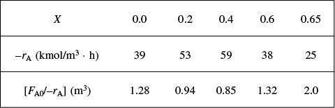
was carried out adiabatically in the liquid phase. The data for this reversible reaction are given in Table E2-5.1. (Example 11.3 shows how the data in Table E2-5.1 were generated.)

Don’t worry how we got this data or why the (1/–rA) looks the way it does; we will see how to construct this table in Chapter 11, Example 11-3. It is real data for a real reaction carried out adiabatically, and the reactor scheme shown below in Figure E2-5.1 is used.

Real Data for a Real Reaction
Calculate the volume of each of the reactors for an entering molar flow rate of n-butane of 50 kmol/hr.
Solution
Taking the reciprocal of –rA and multiplying by FA0, we obtain Table E2-5.2.

(b) For the PFR,
Using Simpson’s three-point formula with ΔX = (0.6 – 0.2)/2 = 0.2, and X1 = 0.2, X2 = 0.4, and X3 = 0.6

(c) For the last reactor and the second CSTR, mole balance on A for the CSTR:
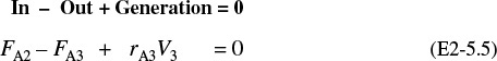
Rearranging
Simplifying

We find from Table E2-5.2 that at X3 = 0.65, then ![]()
V3 = 2 m3 (0.65 – 0.6) = 0.1 m3
A Levenspiel plot of (FA0/–rA) vs. X is shown in Figure E2-5.2.

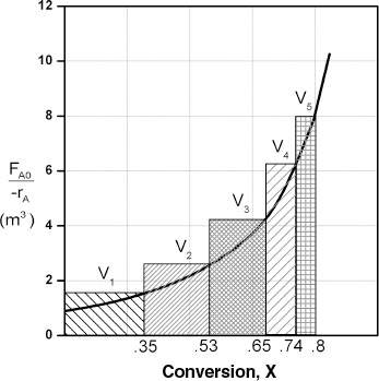
For this adiabatic reaction the three reactors in series resulted in an overall conversion of 65%. The maximum conversion we can achieve is the equilibrium conversion, which is 68%, and is shown by the dashed line in Figure E2-5.2. Recall that at equilibrium, the rate of reaction is zero and an infinite reactor volume is required to reach equilibrium ![]() .
.
Analysis: For exothermic reactions that are not carried out isothermally, the rate usually increases at the start of the reaction because reaction temperature increases. However, as the reaction proceeds the rate eventually decreases as the conversion increases as the reactants are consumed. These two competing effects give the bowed shape of the curve in Figure E2-5.2, which will be discussed in detail in Chapter 12. Under these circumstances, we saw that a CSTR will require a smaller volume than a PFR at low conversions.
2.5.4 Comparing the CSTR and PFR Reactor Volumes and Reactor Sequencing
If we look at Figure E2-5.2, the area under the curve (PFR volume) between X = 0 and X = 0.2, we see that the PFR area is greater than the rectangular area corresponding to the CSTR volume, i.e., VPFR > VCSTR. However, if we compare the areas under the curve between X = 0.6 and X = 0.65, we see that the area under the curve (PFR volume) is smaller than the rectangular area corresponding to the CSTR volume, i.e., VCSTR > VPFR. This result often occurs when the reaction is carried out adiabatically, which is discussed when we look at heat effects in Chapter 11.
Which arrangement is best?

or
In the sequencing of reactors, one is often asked, “Which reactor should go first to give the highest overall conversion? Should it be a PFR followed by a CSTR, or two CSTRs, then a PFR, or...?” The answer is “It depends.” It depends not only on the shape of the Levenspiel plot (FA0/–rA) versus X, but also on the relative reactor sizes. As an exercise, examine Figure E2-5.2 to learn if there is a better way to arrange the two CSTRs and one PFR. Suppose you were given a Levenspiel plot of (FA0/–rA) vs. X for three reactors in series, along with their reactor volumes VCSTR1 = 3 m3, VCSTR2 = 2 m3, and VPFR = 1.2 m3, and were asked to find the highest possible conversion X. What would you do? The methods we used to calculate reactor volumes all apply, except the procedure is reversed and a trial-and-error solution is needed to find the exit overall conversion from each reactor (see Problem P2-5B).
The previous examples show that if we know the molar flow rate to the reactor and the reaction rate as a function of conversion, then we can calculate the reactor volume necessary to achieve a specified conversion. The reaction rate does not depend on conversion alone, however. It is also affected by the initial concentrations of the reactants, the temperature, and the pressure. Consequently, the experimental data obtained in the laboratory and presented in Table 2-1 as –rA as a function of X are useful only in the design of full-scale reactors that are to be operated at the identical conditions as the laboratory experiments (temperature, pressure, and initial reactant concentrations). However, such circumstances are seldom encountered and we must revert to the methods we describe in Chapters 3 and 4 to obtain –rA as a function of X.
It is important to understand that if the rate of reaction is available or can be obtained solely as a function of conversion, –rA = f(X), or if it can be generated by some intermediate calculations, one can design a variety of reactors and combinations of reactors.
Only need –rA = f(X) to size flow reactors
Ordinarily, laboratory data are used to formulate a rate law, and then the reaction rate-conversion functional dependence is determined using the rate law. The preceding sections show that with the reaction rate-conversion relationship, different reactor schemes can readily be sized. In Chapters 3 and 4, we show how we obtain this relationship between reaction rate and conversion from rate law and reaction stoichiometry.
Chapter 3 shows how to find –rA = f(X).
2.6 Some Further Definitions
Before proceeding to Chapter 3, some terms and equations commonly used in reaction engineering need to be defined. We also consider the special case of the plug-flow design equation when the volumetric flow rate is constant.
2.6.1 Space Time
The space time tau, τ, is obtained by dividing the reactor volume by the volumetric flow rate entering the reactor
τ is an important quantity!
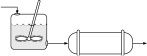
The space time is the time necessary to process one reactor volume of fluid based on entrance conditions. For example, consider the tubular reactor shown in Figure 2-12, which is 20 m long and 0.2 m3 in volume. The dashed line in Figure 2-12 represents 0.2 m3 of fluid directly upstream of the reactor. The time it takes for this fluid to enter the reactor completely is called the space time tau. It is also called the holding time or mean residence time.

Space time or mean residence time τ = V/υ0
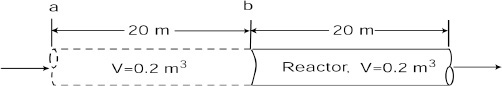
For example, if the reactor volume is 0.2 m3 and the inlet volumetric flow rate is 0.01 m3/s, it would take the upstream equivalent reactor volume (V = 0.2 m3), shown by the dashed lines, a time τ equal to

to enter the reactor (V = 0.2 m3). In other words, it would take 20 s for the fluid molecules at point a to move to point b, which corresponds to a space time of 20 s. We can substitute for FA0 = υ0CA0 in Equations (2-13) and (2-16) and then divide both sides by υ0 to write our mole balance in the following forms:
and
For plug flow, the space time is equal to the mean residence time in the reactor, tm (see Chapter 16). This time is the average time the molecules spend in the reactor. A range of typical processing times in terms of the space time (residence time) for industrial reactors is shown in Table 2-4.
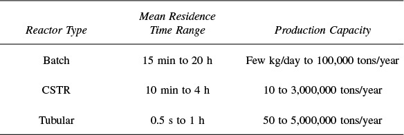
TABLE 2-4 TYPICAL SPACE TIME FOR INDUSTRIAL REACTORS2
2 Trambouze, Landeghem, and Wauquier, Chemical Reactors (Paris: Editions Technip, 1988; Houston: Gulf Publishing Company, 1988), p. 154.
Practical guidelines
Table 2-5 shows an order of magnitude of the space times for six industrial reactions and associated reactors.
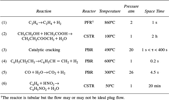
TABLE 2-5 SAMPLE INDUSTRIAL SPACE TIMES3
3 Walas, S. M. Chemical Reactor Data, Chemical Engineering, 79 (October 14, 1985).
Typical industrial reaction space times
Table 2-6 gives typical sizes for batch and CSTR reactors (along with the comparable size of a familiar object) and the costs associated with those sizes. All reactors are glass lined and the prices include heating/cooling jacket, motor, mixer, and baffles. The reactors can be operated at temperatures between 20 and 450°F, and at pressures up to 100 psi.


† Doesn’t include instrumentation costs.
TABLE 2-6 REPRESENTATIVE PFAUDLER CSTR/BATCH REACTOR SIZES AND PRICES†

2.6.2 Space Velocity
The space velocity (SV), which is defined as
might be regarded at first sight as the reciprocal of the space time. However, there can be a difference in the two quantities’ definitions. For the space time, the entering volumetric flow rate is measured at the entrance conditions, but for the space velocity, other conditions are often used. The two space velocities commonly used in industry are the liquid-hourly and gas-hourly space velocities, LHSV and GHSV, respectively. The entering volumetric flow rate, υ0, in the LHSV is frequently measured as that of a liquid feed rate at 60°F or 75°F, even though the feed to the reactor may be a vapor at some higher temperature. Strange but true. The gas volumetric flow rate, υ0, in the GHSV is normally reported at standard temperature and pressure (STP).
Example 2–6 Reactor Space Times and Space Velocities
Calculate the space time, τ, and space velocities for the reactor in Examples 2-1 and 2-3 for an entering volumetric flow rate of 2 dm3/s.
Solution
The entering volumetric flow is 2 dm3/s (0.002 m3/s).
From Example 2-1, the CSTR volume was 6.4 m3 and the corresponding space time, τ, and space velocity, SV are

It takes 0.89 hours to put 6.4 m3 into the reactor.
From Example 2-3, the PFR volume was 2.165 m3, and the corresponding space time and space velocity are

Analysis: This example gives an important industrial concept. These space times are the times for each of the reactors to take the volume of fluid equivalent to one reactor volume and put it into the reactor.
Summary
In these last examples we have seen that in the design of reactors that are to be operated at conditions (e.g., temperature and initial concentration) identical to those at which the reaction rate data were obtained, we can size (determine the reactor volume) both CSTRs and PFRs alone or in various combinations. In principle, it may be possible to scale up a laboratory-bench or pilot-plant reaction system solely from knowledge of –rA as a function of X or CA. However, for most reactor systems in industry, a scale-up process cannot be achieved in this manner because knowledge of –rA solely as a function of X is seldom, if ever, available under identical conditions. By combining the information in Chapters 3 and 4, we shall see how we can obtain –rA = f(X) from information obtained either in the laboratory or from the literature. This relationship will be developed in a two-step process. In Step 1, we will find the rate law that gives the rate as a function of concentration (Chapter 3) and in Step 2, we will find the concentrations as a function of conversion (Chapter 4). Combining Steps 1 and 2 in Chapters 3 and 4, we obtain –rA = f(X). We can then use the methods developed in this chapter, along with integral and numerical methods, to size reactors.
Coming attractions Chapters 3 and 4
The CRE Algorithm
• Mole Balance, Ch 1
• Rate Law, Ch 3
• Stoichiometry, Ch 4
• Combine, Ch 5
• Evaluate, Ch 5
• Energy Balance, Ch 11
Summary
1. The conversion X is the moles of A reacted per mole of A fed.
For reactors in series with no side streams, the conversion at point i is
2. In terms of the conversion, the differential and integral forms of the reactor design equations become:

3. If the rate of disappearance of A is given as a function of conversion, the following graphical techniques can be used to size a CSTR and a plug-flow reactor.
A. Graphical Integration Using Levenspiel Plots

The PFR integral could also be evaluated by
B. Numerical Integration
See Appendix A.4 for quadrature formulas such as the five-point quadrature formula with ΔX = 0.8/4 of five equally spaced points, X1 = 0, X2 = 0.2, X3 = 0.4, X4 = 0.6, and X5 = 0.8.
4. Space time, τ, and space velocity, SV, are given by
1. Web P2–1A Reactor Sizing for Reversible Reactions
2. Web P2–2A Puzzle Problem “What’s Wrong with this Solution?”
• Learning Resources
1. Summary Notes for Chapter 2
2. Web Module
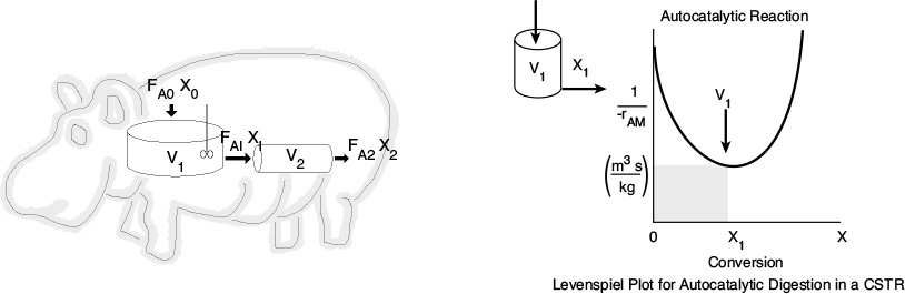
Hippopotamus Digestive System
3. Interactive Computer Games
Reactor Staging

4. Solved Problems
A. CDP 2-AB More CSTR and PFR Calculations–No Memorization
• FAQ (Frequently Asked Questions)
• Professional Reference Shelf
Questions and Problems
The subscript to each of the problem numbers indicates the level of difficulty: A, least difficult; D, most difficult.
Questions
Q2-1
(a) Without referring back, make a list of the most important items you learned in this chapter.
(b) What do you believe was the overall purpose of the chapter?
Before solving the problems, state or sketch qualitatively the expected results or trends.
Q2-2 Go to the Web site www.engr.ncsu.edu/learningstyles/ilsweb.html.
(a) Take the Inventory of Learning Style test, and record your learning style according to the Solomon/Felder inventory.
Global/Sequential_____
Active/Reflective_____
Visual/Verbal_____
Sensing/Intuitive_____
(b) After checking the CRE Web site, www.umich.edu/~elements/asyLearn/learningstyles.htm, suggest two ways to facilitate your learning style in each of the four categories.
(a) Revisit Examples 2-1 through 2-3. How would your answers change if the flow rate, FA0, were cut in half? If it were doubled? What conversion can be achieved in a 4.5 m3 PFR and in a 4.5 m3 CSTR?
(b) Revisit Example 2-2. Being a company about to go bankrupt, you can only afford a 2.5 m3 CSTR. What conversion can you achieve?
(c) Revisit Example 2-3. What conversion could you achieve if you could convince your boss, Dr. Pennypincher, to spend more money to buy a 1.0 m3 PFR to attach to a 2.40 CSTR?
(d) Revisit Example 2-4. How would your answers change if the two CSTRs (one 0.82 m3 and the other 3.2 m3) were placed in parallel with the flow, FA0, divided equally between the reactors.
(e) Revisit Example 2-5. (1) What would be the reactor volumes if the two intermediate conversions were changed to 20% and 50%, respectively? (2) What would be the conversions, X1, X2, and X3, if all the reactors had the same volume of 100 dm3 and were placed in the same order? (3) What is the worst possible way to arrange the two CSTRs and one PFR?
(f) Revisit Example 2-6. If the term ![]() is 2 seconds for 80% conversion, how much fluid (m3/min) can you process in a 3 m3 reactor?
is 2 seconds for 80% conversion, how much fluid (m3/min) can you process in a 3 m3 reactor?
P2-2A ICG Staging. Download the Interactive Computer Game (ICG) from the CRE Web site. Play this game and then record your performance number, which indicates your mastery of the material. Your professor has the key to decode your performance number. Note: To play this game you must have Windows 2000 or a later version.
ICG Reactor Staging Performance #_________________________________________________

P2-3B You have two CSTRs and two PFRs, each with a volume of 1.6 m3. Use Figure 2-2B on page 41 to calculate the conversion for each of the reactors in the following arrangements.
(a) Two CSTRs in series. (Ans.: X1 = 0.435, X2 = 0.66)
(b) Two PFRs in series.
(c) Two CSTRs in parallel with the feed, FA0, divided equally between the two reactors.
(d) Two PFRs in parallel with the feed divided equally between the two reactors.
(e) Caution: Part (e) is a C level problem. A CSTR and a PFR in parallel with the flow equally divided. Calculate the overall conversion, Xov
(f) A PFR followed by a CSTR.
(g) A CSTR followed by a PFR. ( Ans.: XCSTR = 0.435 and XPFR = 0.71)
(h) A PFR followed by two CSTRs. Is this arrangement a good arrangement or is there a better one?
P2-4B The exothermic reaction of stillbene (A) to form the economically important trospophene (B) and methane (C), i.e.,
was carried out adiabatically and the following data recorded:
The entering molar flow rate of A was 300 mol/min.
(a) What are the PFR and CSTR volumes necessary to achieve 40% conversion? (VPFR = 72 dm3, VCSTR = 24 dm3)
(b) Over what range of conversions would the CSTR and PFR reactor volumes be identical?
(c) What is the maximum conversion that can be achieved in a 105-dm3 CSTR?
(d) What conversion can be achieved if a 72-dm3 PFR is followed in series by a 24-dm3 CSTR?
(e) What conversion can be achieved if a 24-dm3 CSTR is followed in a series by a 72-dm3 PFR?
(f) Plot the conversion and rate of reaction as a function of PFR reactor volume up to a volume of 100 dm3.
P2-5B The financially important reaction to produce the valuable product B (not the real name) was carried out in Jesse Pinkman’s garage. This breaking bad, fly-by-night company is on a shoestring budget and has very little money to purchase equipment. Fortunately, cousin Bernie has a reactor surplus company and get reactors for them. The reaction
takes place in the liquid phase. Below is the Levenspiel plot for this reaction.
You have up to $10,000 to use to purchase reactors from those given below.

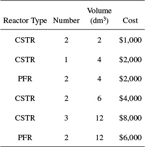
What reactors do you choose, how do you arrange them, and what is the highest conversion you can get for $10,000? Approximately what is the corresponding highest conversion with your arrangement of reactors?
Scheme and sketch your reactor volumes.
P2-6B Read the Web Module “Chemical Reaction Engineering of Hippopotamus Stomach” on the CRE Web site.

(a) Write five sentences summarizing what you learned from the Web Module.
(b) Work problems (1) and (2) in the Hippo Web Module.
(c) The hippo has picked up a river fungus, and now the effective volume of the CSTR stomach compartment is only 0.2 m3. The hippo needs 30% conversion to survive. Will the hippo survive?
(d) The hippo had to have surgery to remove a blockage. Unfortunately, the surgeon, Dr. No, accidentally reversed the CSTR and the PFR during the operation. Oops!! What will be the conversion with the new digestive arrangement? Can the hippo survive?
P2-7B The adiabatic exothermic irreversible gas-phase reaction
is to be carried out in a flow reactor for an equimolar feed of A and B. A Levenspiel plot for this reaction is shown in Figure P2-7B.

(a) What PFR volume is necessary to achieve 50% conversion?
(b) What CSTR volume is necessary to achieve 50% conversion?
(c) What is the volume of a second CSTR added in series to the first CSTR (Part b) necessary to achieve an overall conversion of 80%? (Ans.: VCSTR = 1.5 × 10⁵ m3 )
(d) What PFR volume must be added to the first CSTR (Part b) to raise the conversion to 80%?
(e) What conversion can be achieved in a 6 × 10⁴ m3 CSTR? In a 6 × 10⁴ m3 PFR?
(f) Think critically (cf. Preface, Section I, page xxviii) to critique the answers (numbers) to this problem.
P2-8A Estimate the reactor volumes of the two CSTRs and the PFR shown in the photo in Figure 2-9. [Hint: Use the dimensions of the door as a scale.]
P2-9D Don’t calculate anything. Just go home and relax.
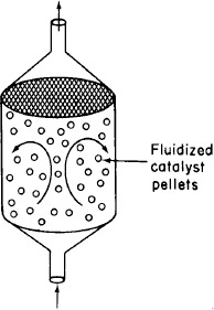
P2-10C The curve shown in Figure 2-1 is typical of a reaction carried out isothermally, and the curve shown in Figure P2-10B (see Example 11-3) is typical of a gas-solid catalytic exothermic reaction carried out adiabatically.
(a) Assuming that you have a fluidized CSTR and a PBR containing equal weights of catalyst, how should they be arranged for this adiabatic reaction? Use the smallest amount of catalyst weight to achieve 80% conversion of A.
(b) What is the catalyst weight necessary to achieve 80% conversion in a fluidized CSTR? (Ans.: W = 23.2 kg of catalyst)
(c) What fluidized CSTR weight is necessary to achieve 40% conversion?
(d) What PBR weight is necessary to achieve 80% conversion?
(e) What PBR weight is necessary to achieve 40% conversion?
(f) Plot the rate of reaction and conversion as a function of PBR catalyst weight, W.
Additional information: FA0 = 2 mol/s.
• Additional Homework Problems on the CRE Web Site
CDP2-AA An ethical dilemma as to how to determine the reactor size in a competitor’s chemical plant. [ECRE, 2nd Ed. P2-18B]
Supplementary Reading
Further discussion of the proper staging of reactors in series for various rate laws, in which a plot of –1/rA versus X is given, may or may not be presented in
BURGESS, THORNTON W., The Adventures of Poor Mrs. Quack, New York: Dover Publications, Inc., 1917.
KARRASS, CHESTER L., Effective Negotiating: Workbook and Discussion Guide, Beverly Hills, CA: Karrass Ltd., 2004.
LEVENSPIEL, O., Chemical Reaction Engineering, 3rd ed. New York: Wiley, 1999, Chapter 6, pp. 139-156.