
Chapter 5
Ordered Algebraic Structures
This chapter presents a hierarchy of concepts from abstract algebra, starting with semigroups and ending with rings and modules. We then combine algebraic concepts with the notion of total ordering. When ordered algebraic structures are Archimedean, we can define an efficient algorithm for finding quotient and remainder. Quotient and remainder in turn lead to a generalized version of Euclid’s algorithm for the greatest common divisor. We briefly treat concept-related logical notions, such as consistency and independence. We conclude with a discussion of computer integer arithmetic.
5.1 Basic Algebraic Structures
An element is called an identity element of a binary operation if, when combined with any other element as the first or second argument, the operation returns the other element:
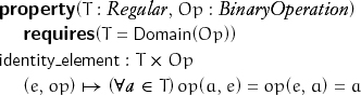
Lemma 5.1 An identity element is unique:
identity_element(e, op) ![]() identity_element (e′, op)
identity_element (e′, op) ![]() e = e′
e = e′
The empty string is the identity element of string concatenation. The matrix ![]() is the multiplicative identity of 2 × 2 matrices, while
is the multiplicative identity of 2 × 2 matrices, while ![]() is their additive identity.
is their additive identity.
A transformation is called an inverse operation with respect to a given element (usually the identity of the binary operation) if it satisfies the following:
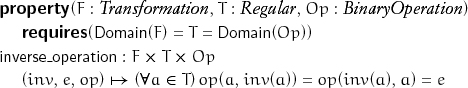
Lemma 5.2 n3 is the multiplicative inverse modulo 5 of a positive integer n ≠ 0.
A binary operation is commutative if its result is the same when its arguments are interchanged:
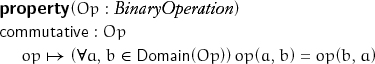
Composition of transformations is associative but not commutative.
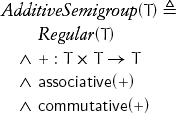
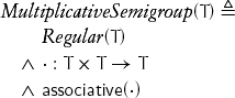
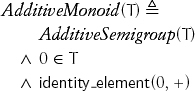
A set with an associative operation is called a semigroup. Since, as we remarked in Chapter 3, + is always used to denote an associative, commutative operation, a type with + is called an additive semigroup:
Multiplication is sometimes not commutative. Consider, for example, matrix multiplication.
We use the following notation:
![]()
A semigroup with an identity element is called a monoid. The additive identity element is denoted by 0, which leads to the definition of an additive monoid:
We use the following notation:
![]()
Non-negative reals are an additive monoid, as are matrices with natural numbers as their coefficients.
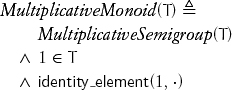
The multiplicative identity element is denoted by 1, which leads to the definition of a multiplicative monoid:
We use the following notation:
![]()
Matrices with integer coefficients are a multiplicative monoid.
A monoid with an inverse operation is called a group. If an additive monoid has an inverse, it is denoted by unary –, and there is a derived operation called subtraction, denoted by binary –. That leads to the definition of an additive group:
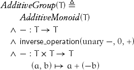
Matrices with integer coefficients are an additive group.
Lemma 5.3 In an additive group, –0 = 0.
Just as there is a concept of additive group, there is a corresponding concept of multiplicative group. In this concept the inverse is called multiplicative inverse, and there is a derived operation called division, denoted by binary / :
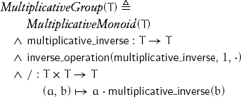
multiplicative_inverse(x) is written as x–1.
The set {cos θ + i sin θ} of complex numbers on the unit circle is a commutative multiplicative group. A unimodular group GLn![]() (n × n matrices with integer coefficients with determinant equal to ±1) is a noncommutative multiplicative group.
(n × n matrices with integer coefficients with determinant equal to ±1) is a noncommutative multiplicative group.
Two concepts can be combined on the same type with the help of axioms connecting their operations. When both + and · are present on a type, they are interrelated with axioms defining a semiring:
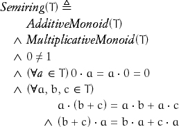
The axiom about multiplication by 0 is called the annihilation property. The final axiom connecting + and · is called distributivity.
Matrices with non-negative integer coefficients constitute a semiring.
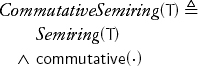
Non-negative integers constitute a commutative semiring.
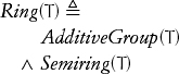
Matrices with integer coefficients constitute a ring.
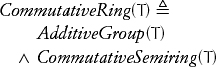
Integers constitute a commutative ring; polynomials with integer coefficients constitute a commutative ring.
A relational concept is a concept defined on two types. Semimodule is a relational concept that connects an additive monoid and a commutative semiring:
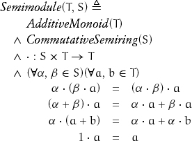
If Semimodule(T, S), we say that T is a semimodule over S. We borrow terminology from vector spaces and call elements of T vectors and elements of S scalars. For example, polynomials with non-negative integer coefficients constitute a semimodule over non-negative integers.
Theorem 5.1 AdditiveMonoid(T) ![]() Semimodule(T,
Semimodule(T, ![]() ), where scalar multiplication is defined as
), where scalar multiplication is defined as ![]()
Proof: It follows trivially from the definition of scalar multiplication together with associativity and commutativity of the monoid operation. For example,
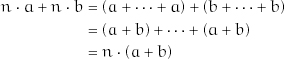
Using power from Chapter 3 allows us to implement multiplication by an integer in log2 n steps.
Strengthening the requirements by replacing the additive monoid with an additive group and replacing the semiring with a ring transforms a semimodule into a module:
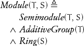
Lemma 5.4 Every additive group is a module over integers with an appropriately defined scalar multiplication.
Computer types are often partial models of concepts. A model is called partial when the operations satisfy the axioms where they are defined but are not everywhere defined. For example, the result of concatenation of strings may not be representable, because of memory limitations, but concatenation is associative whenever it is defined.
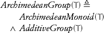
5.2 Ordered Algebraic Structures
When a total ordering is defined on the elements of a structure in such a way that the ordering is consistent with the structure’s algebraic properties, it is the natural total ordering for the structure:
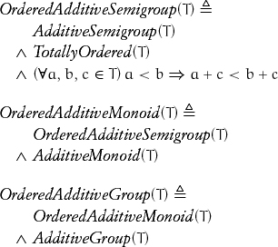
Lemma 5.5 In an ordered additive semigroup, a < b ![]() c < d
c < d ![]() a + c < b + d.
a + c < b + d.
Lemma 5.6 In an ordered additive monoid viewed as a semimodule over natural numbers, a > 0 ![]() n > 0
n > 0 ![]() na > 0.
na > 0.
Lemma 5.7 In an ordered additive group, a < b ![]() –b < –a.
–b < –a.
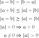
Total ordering and negation allow us to define absolute value:
template<typename T>
requires(OrderedAdditiveGroup(T))
T abs(const T& a)
{
if (a < T(0)) return -a;
else return a;
}
The following lemma captures an important property of abs.
Lemma 5.8 In an ordered additive group, a < 0 ![]() 0< –a.
0< –a.
We use the notation |a| for the absolute value of a. Absolute value satisfies the following properties.
5.3 Remainder
We saw that repeated addition in an additive monoid induces multiplication by a non-negative. In an additive group, this algorithm can be inverted, obtaining division by repeated subtraction on elements of the form a = nb, where b divides a. To extend this to division with remainder for an arbitrary pair of elements, we need ordering. The ordering allows the algorithm to terminate when it is no longer possible to subtract. As we shall see, it also enables an algorithm to take a logarithmic number of steps. The subtraction operation does not need to be defined everywhere; it is sufficient to have a partial subtraction called cancellation, where a–b is only defined when b does not exceed a:
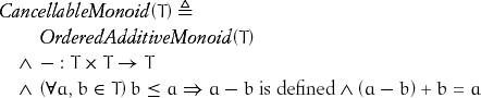
We write the axiom as (a – b) + b = a instead of (a + b) – b = a to avoid overflow in partial models of CancellableMonoid:
template<typename T>
requires(CancellableMonoid(T))
T slow_remainder(T a, T b)
{
// Precondition: a ≥ 0 ![]() b > 0
b > 0
while (b <= a) a = a - b;
return a;
}
The concept CancellableMonoid is not strong enough to prove termination of slow_remainder. For example, slow_remainder does not always terminate for polynomials with integer coefficients, ordered lexicographically.
Exercise 5.1 Give an example of two polynomials with integer coefficients for which the algorithm does not terminate.
To ensure that the algorithm terminates, we need another property, called the Axiom of Archimedes:[1]
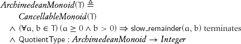
Observe that termination of an algorithm is a legitimate axiom; in this case it is equivalent to
(∃n ![]() QuotientType(T)) a – n · b < b
QuotientType(T)) a – n · b < b
While the Axiom of Archimedes is usually given as “there exists an integer n such that a < n · b,” our version works with partial Archimedean monoids where n · b might overflow. The type function QuotientType returns a type large enough to represent the number of iterations performed by slow_remainder.
Lemma 5.10 The following are Archimedean monoids: integers, rational numbers, binary fractions ![]() , ternary fractions
, ternary fractions ![]() , and real numbers.
, and real numbers.
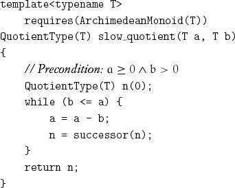
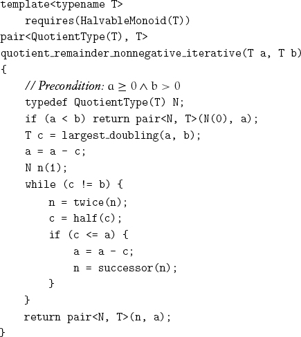
We can trivially adapt the code of slow_remainder to return the quotient:
Repeated doubling leads to the logarithmic-complexity power algorithm. A related algorithm is possible for remainder.[2] Let us derive an expression for the remainder u from dividing a by b in terms of the remainder v from dividing a by 2b:
a = n(2b)+ v
Since the remainder v must be less than the divisor 2b, it follows that
![]()
That leads to the following recursive procedure:
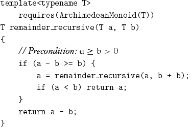
Testing a – b ≥ b rather than a ≥ b + b avoids overflow of b + b.
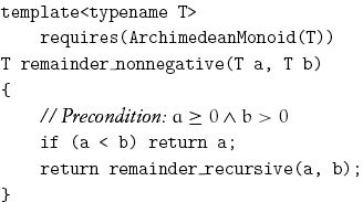
Exercise 5.2 Analyze the complexity of remainder_nonnegative.
Floyd and Knuth [1990] give a constant-space algorithm for remainder on Archimedean monoids that performs about 31% more operations than remainder nonnegative, but when we can divide by 2 an algorithm exists that does not increase the operation count.[3] This is likely to be possible in many situations. For example, while the general k-section of an angle by ruler and compass cannot be done, the bisection is trivial.
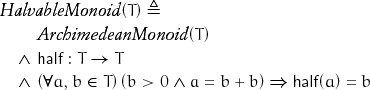
Observe that half needs to be defined only for “even” elements.
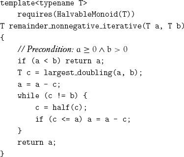
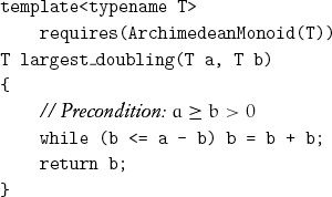
where largest_doubling is defined by the following procedure:
The correctness of remainder_nonnegative_iterative depends on the following lemma.
Lemma 5.11 The result of doubling a positive element of a halvable monoid k times may be halved k times.
We would only need remainder_nonnegative if we had an Archimedean monoid that was not halvable. The examples we gave—line segments in Euclidean geometry, rational numbers, binary and ternary fractions—are all halvable.
Project 5.1 Are there useful models of Archimedean monoids that are not halvable monoids?
5.4 Greatest Common Divisor
For a ≥ 0 and b > 0 in an Archimedean monoid T, we define divisibility as follows:
b divides a ![]() (∃n
(∃n ![]() QuotientType(T)) a = nb
QuotientType(T)) a = nb
Lemma 5.12 In an Archimedean monoid T with positive x, a, b:
- b divides a
 remainder_nonnegative(a, b) = 0
 - b divides a
 b ≤ a
b ≤ a - a > b
 x divides a x divides b x divides (a – b)
 - x divides a x divides b x divides remainder_nonnegative(a, b)
The greatest common divisor of a and b, denoted by gcd(a, b), is a divisor of a and b that is divisible by any other common divisor of a and b.[4]
Lemma 5.13 In an Archimedean monoid, the following hold for positive x, a, b:
- gcd is commutative
- gcd is associative
- x divides a x divides b x ≤ gcd(a, b)
- gcd(a, b) is unique
- gcd(a, a) = a
- a > b gcd(a, b) = gcd(a – b, b)
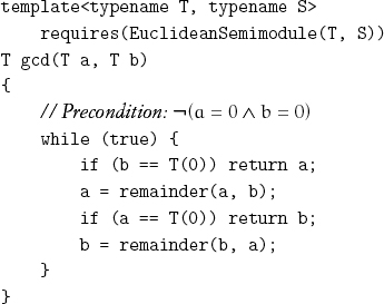
The previous lemmas immediately imply that if the following algorithm terminates, it returns the gcd of its arguments:[5]
Lemma 5.14 It always terminates for integers and rationals.
There are types for which it does not always terminate. In particular, it does not always terminate for real numbers; specifically, it does not terminate for input of ![]() and 1. The proof of this fact depends on the following two lemmas:
and 1. The proof of this fact depends on the following two lemmas:
![]()
Lemma 5.16 If the square of an integer n is even, n is even.
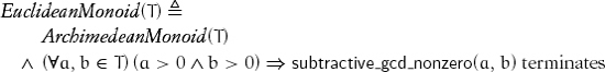
Theorem 5.2 subtractive_gcd_nonzero(![]() , 1) does not terminate.
, 1) does not terminate.
Proof: Suppose that subtractive_gcd_nonzero(![]() , 1) terminates, returning d. Let m =
, 1) terminates, returning d. Let m = ![]() and
and ![]() ; by Lemma 5.15, m and n have no common factors greater than 1.
; by Lemma 5.15, m and n have no common factors greater than 1. ![]() , so m2 = 2n2; m is even; for some integer u, m = 2u. 4u2 = 2n2, so n2 = 2u2; n is even. Both m and n are divisible by 2; a contradiction.[6]
, so m2 = 2n2; m is even; for some integer u, m = 2u. 4u2 = 2n2, so n2 = 2u2; n is even. Both m and n are divisible by 2; a contradiction.[6]
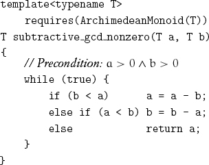
A Euclidean monoid is an Archimedean monoid where subtractive_gcd_nonzero always terminates:
Lemma 5.17 Every Archimedean monoid with a smallest positive element is Euclidean.
Lemma 5.18 The rational numbers are a Euclidean monoid.
It is straightforward to extend subtractive_gcd_nonzero to the case in which one of its arguments is zero, since any b ≠ 0 divides the zero of the monoid:
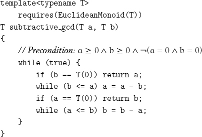
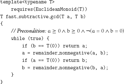
Each of the inner while statements in subtractive_gcd is equivalent to a call of slow_remainder. By using our logarithmic remainder algorithm, we speed up the case when a and b are very different in magnitude while relying only on primitive subtraction on type T:
The concept of Euclidean monoid gives us an abstract setting for the original Euclid algorithm, which was based on repeated subtraction.
5.5 Generalizing gcd
We can use fast_subtractive_gcd with integers because they constitute a Euclidean monoid. For integers, we could also use the same algorithm with the built-in remainder instead of remainder_nonnegative. Furthermore, the algorithm works for certain non-Archimedean domains, provided that they possess a suitable remainder function. For example, the standard long-division algorithm easily extends from decimal integers to polynomials over reals.[7] Using such a remainder, we can compute the gcd of two polynomials.
Abstract algebra introduces the notion of a Euclidean ring (also known as a Euclidean domain) to accommodate such uses of the Euclid algorithm.[8] However, the requirements of semiring suffice:
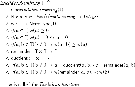
w is called the Euclidean function.
Lemma 5.19 In a Euclidean semiring, a · b = 0 ![]() a = 0
a = 0 ![]() b = 0.
b = 0.
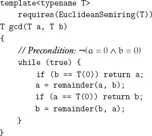
Observe that instead of using remainder_nonnegative, we use the remainder function defined by the type. The fact that w decreases with every application of remainder ensures termination.
Lemma 5.20 gcd terminates on a Euclidean semiring.
In a Euclidean semiring, quotient returns an element of the semiring. This precludes its use in the original setting of Euclid: determining the common measure of any two commensurable quantities. For example, gcd ![]() . We can unify the original setting and the modern setting with the concept Euclidean semimodule, which allows quotient to return a different type and takes the termination of gcd as an axiom:
. We can unify the original setting and the modern setting with the concept Euclidean semimodule, which allows quotient to return a different type and takes the termination of gcd as an axiom:
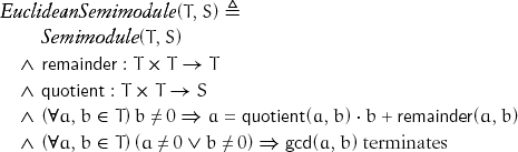
where gcd is defined as
Since every commutative semiring is a semimodule over itself, this algorithm can be used even when quotient returns the same type, as with polynomials over reals.
5.6 Stein gcd
In 1961 Josef Stein discovered a new gcd algorithm for integers that is frequently faster than Euclid’s algorithm [Stein, 1967]. His algorithm depends on these two familiar properties:
![]()
together with these additional properties that for all a > b > 0:
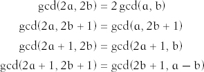
Exercise 5.3 Implement Stein gcd for integers, and prove its termination.
While it might appear that Stein gcd depends on the binary representation of integers, the intuition that 2 is the smallest prime integer allows generalizing it to other domains by using smallest primes in these domains; for example, the monomial x for polynomials[9] or 1 + i for Gaussian integers.[10] Stein gcd could be used in rings that are not Euclidean.[11]
Project 5.2 Find the correct general setting for Stein gcd.
5.7 Quotient
The derivation of fast quotient and remainder exactly parallels our earlier derivation of fast remainder. We derive an expression for the quotient m and remainder u from dividing a by b in terms of the quotient n and remainder v from dividing a by 2b:
a = n(2b)+ v
Since the remainder v must be less than the divisor 2b, it follows that
![]()
and
![]()
This leads to the following code:
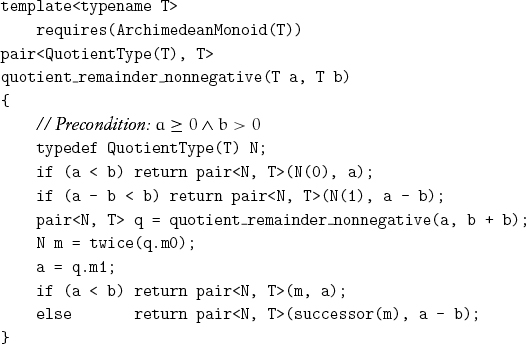
When “halving” is available, we obtain the following:
5.8 Quotient and Remainder for Negative Quantities
The definition of quotient and remainder used by many computer processors and programming languages handles negative quantities incorrectly. An extension of our definitions for an Archimedean monoid to an Archimedean group T must satisfy these properties, where b ≠ 0:
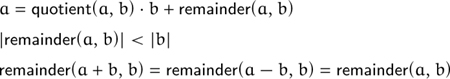
The final property is equivalent to the classical mathematical definition of congruence.[12] While books on number theory usually assume b > 0, we can consistently extend remainder to b < 0. These requirements are not satisfied by implementations that truncate quotient toward zero, thus violating our third requirement.[13] In addition to violating the third requirement, truncation is an inferior way of rounding because it sends twice as many values to zero as to any other integer, thus leading to a nonuniform distribution.
Given a remainder procedure rem and a quotient-remainder procedure quo_rem satisfying our three requirements for non-negative inputs, we can write adapter procedures that give correct results for positive or negative inputs. These adapter procedures will work on an Archimedean group:
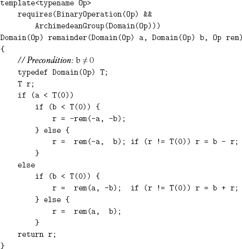
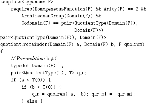
Lemma 5.21 remainder and quotient_remainder satisfy our requirements when their functional parameters satisfy the requirements for positive arguments.
5.9 Concepts and Their Models
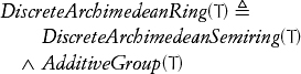
We have been using integer types since Chapter 2 without formally defining the concept. Building on the ordered algebraic structures defined earlier in this chapter, we can formalize our treatment of integers. First, we define discrete Archimedean semiring:
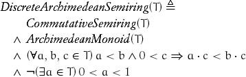
Discreteness refers to the last property: There is no element between 0 and 1.
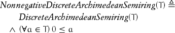
A discrete Archimedean semiring might have negative elements. The related concept that does not have negative elements is
A discrete Archimedean semiring lacks additive inverses; the related concept with additive inverses is
Two types T and T′ are isomorphic if it is possible to write conversion functions from T to T′ and from T′ to T that preserve the procedures and their axioms.
A concept is univalent if any types satisfying it are isomorphic. The concept NonnegativeDiscreteArchimedeanSemiring is univalent; types satisfying it are isomorphic to ![]() , the natural numbers.[14] DiscreteArchimedeanRing is univalent; types satisfying it are isomorphic to
, the natural numbers.[14] DiscreteArchimedeanRing is univalent; types satisfying it are isomorphic to ![]() , the integers. As we have seen here, adding axioms reduces the number of models of a concept, so that one quickly reaches the point of univalency.
, the integers. As we have seen here, adding axioms reduces the number of models of a concept, so that one quickly reaches the point of univalency.
This chapter proceeds deductively, from more general to more specific concepts, by adding more operations and axioms. The deductive approach statically presents a taxonomy of concepts and affiliated theorems and algorithms. The actual process of discovery proceeds inductively, starting with concrete models, such as integers or reals, and then removing operations and axioms to find the weakest concept to which interesting algorithms apply.
When we define a concept, the independence and consistency of its axioms must be verified, and its usefulness must be demonstrated.
A proposition is independent from a set of axioms if there is a model in which all the axioms are true, but the proposition is false. For example, associativity and commutativity are independent: String concatenation is associative but not commutative, while the average of two values ![]() is commutative but not associative. A proposition is dependent or provable from a set of axioms if it can be derived from them.
is commutative but not associative. A proposition is dependent or provable from a set of axioms if it can be derived from them.
A concept is consistent if it has a model. Continuing our example, addition of natural numbers is associative and commutative. A concept is inconsistent if both a proposition and its negation can be derived from its axioms. In other words, to demonstrate consistency, we construct a model; to demonstrate inconsistency, we derive a contradiction.
A concept is useful if there are useful algorithms for which this is the most abstract setting. For example, parallel out-of-order reduction applies to any associative, commutative operation.
5.10 Computer Integer Types
Computer instruction sets typically provide partial representations of natural numbers and integers. For example, a bounded unsigned binary integer type, Un, where n = 8, 16, 32, 64, ..., is an unsigned integer type capable of representing a value in the interval [0, 2n); a bounded signed binary integer type, Sn, where n = 8, 16, 32, 64, ..., is a signed integer type capable of representing a value in the interval [–2n–1, 2n–1). Although these types are bounded, typical computer instructions provide total operations on them because the results are encoded as a tuple of bounded values.
Instructions on bounded unsigned types with signatures like these usually exist:
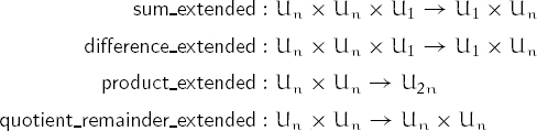
Observe that U2n can be represented as Un × Un (a pair of Un). Programming languages that provide full access to these hardware operations make it possible to write efficient and abstract software components involving integer types.
Project 5.3 Design a family of concepts for bounded unsigned and signed binary integers. A study of the instruction sets for modern computer architectures shows the functionality that should be encompassed. A good abstraction of these instruction sets is provided by MMIX [Knuth, 2005].
5.11 Conclusions
We can combine algorithms and mathematical structures into a seamless whole by describing algorithms in abstract terms and adjusting theories to fit algorithmic requirements. The mathematics and algorithms in this chapter are abstract restatements of results that are more than two thousand years old.