
Chapter 3
Associative Operations
This chapter discusses associative binary operations. Associativity allows regrouping the adjacent operations. This ability to regroup leads to an efficient algorithm for computing powers of the binary operation. Regularity enables a variety of program transformations to optimize the algorithm. We then use the algorithm to compute linear recurrences, such as Fibonacci numbers, in logarithmic time.
3.1 Associativity
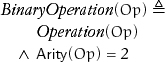
A binary operation is an operation with two arguments:
The binary operations of addition and multiplication are central to mathematics. Many more are used, such as min, max, conjunction, disjunction, set union, set intersection, and so on. All these operations are associative:
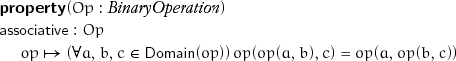
There are, of course, nonassociative binary operations, such as subtraction and division.
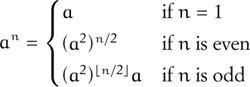
When a particular associative binary operation op is clear from the context, we often use implied multiplicative notation by writing ab instead of op(a, b). Because of associativity, we do not need to parenthesize an expression involving two or more applications of op, because all the groupings are equivalent: (... (a0a1) ... ) an–1 = ... = a0(... (an–2an–1) ... ) = a0a1 ... an–1. When a0 = a1 = ... = an–1 = a, we write an: the nth power of a.
Lemma 3.1 anam = aman = an+m (powers of the same element commute)
It is not, however, always true that (ab)n = anbn. This condition holds only when the operation is commutative.
If f and g are transformations on the same domain, their composition, g ο f, is a transformation mapping x to g(f(x)).
Lemma 3.3 The binary operation of composition is associative.
If we choose some element a of the domain of an associative operation op and consider the expression op(a, x) as a unary operation with formal parameter x, we can think of a as the transformation “multiplication by a.” This justifies the use of the same notation for powers of a transformation, fn, and powers of an element under an associative binary operation, an. This duality allows us to use an algorithm from the previous chapter to prove an interesting theorem about powers of an associative operation. An element x has finite order under an associative operation if there exist integers 0 < n < m such that xn = xm. An element x is an idempotent element under an associative operation if x = x2.
Theorem 3.1 An element of finite order has an idempotent power (Frobenius [1895]).
Proof: Assume that x is an element of finite order under an associative operation op. Let g(z) = op(x, z). Since x is an element of finite order, its orbit under g has a cycle. By its postcondition,
collision_point(x, g) = gn(x) = g2n+1(x)
for some n ≥ 0. Thus
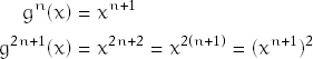
and xn+1 is the idempotent power of x.
Lemma 3.4 collision_point_nonterminating_orbit can be used in the proof.
3.2 Computing Powers
An algorithm to compute an for an associative operation op will take a, n, and op as parameters. The type of a is the domain of op; n must be of an integer type. Without the assumption of associativity, two algorithms compute power from left to right and right to left, respectively:
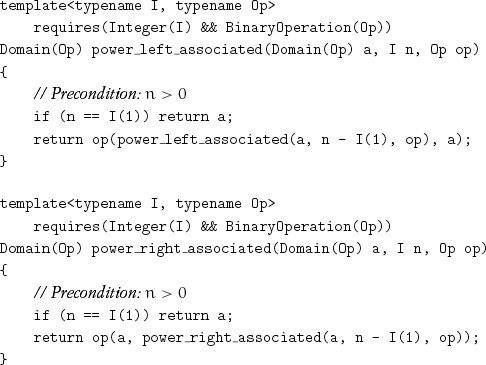
The algorithms perform n – 1 operations. They return different results for a nonassociative operation. Consider, for example, raising 1 to the 3rd power with the operation of subtraction.
When both a and n are integers, and if the operation is multiplication, both algorithms give us exponentiation; if the operation is addition, both give us multiplication. The ancient Egyptians discovered a faster multiplication algorithm that can be generalized to computing powers of any associative operation.[1]
Since associativity allows us to freely regroup operations, we have
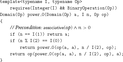
Let us count the number of operations performed by power_0 for an exponent of n. The number of recursive calls is ![]() log2n
log2n![]() . Let υ be the number of 1s in the binary representation of n. Each recursive call performs an operation to square a. Also, υ – 1 of the calls perform an extra operation. So the number of operations is
. Let υ be the number of 1s in the binary representation of n. Each recursive call performs an operation to square a. Also, υ – 1 of the calls perform an extra operation. So the number of operations is
![]() log2n
log2n![]() + (v – 1)≤ 2
+ (v – 1)≤ 2![]() log2n
log2n![]()
For n = 15, ![]() log2n
log2n![]() = 3 and the number of 1s is four, so the formula gives six operations. A different grouping gives a15 = (a3)5, where a3 takes two operations and a5 takes three operations, for a total of five. There are also faster groupings for other exponents, such as 23, 27, 39, and 43.[2]
= 3 and the number of 1s is four, so the formula gives six operations. A different grouping gives a15 = (a3)5, where a3 takes two operations and a5 takes three operations, for a total of five. There are also faster groupings for other exponents, such as 23, 27, 39, and 43.[2]
Since power_left_associated does n – 1 operations and power_0 does at most 2![]() log2n
log2n![]() operations, it might appear that for very large n, power_0 will always be much faster. This is not always the case. For example, if the operation is multiplication of univariate polynomials with arbitrary-precision integer coefficients, power_left_associated is faster.[3] Even for this simple algorithm, we do not know how to precisely specify the complexity requirements that determine which of the two is better.
operations, it might appear that for very large n, power_0 will always be much faster. This is not always the case. For example, if the operation is multiplication of univariate polynomials with arbitrary-precision integer coefficients, power_left_associated is faster.[3] Even for this simple algorithm, we do not know how to precisely specify the complexity requirements that determine which of the two is better.
The ability of power_0 to handle very large exponents, say 10300, makes it crucial for cryptography.[4]
3.3 Program Transformations
power_0 is a satisfactory implementation of the algorithm and is appropriate when the cost of performing the operation is considerably larger than the overhead of the function calls caused by recursion. In this section we derive the iterative algorithm that performs the same number of operations as power_0, using a sequence of program transformations that can be used in many contexts.[5] For the rest of the book, we only show final or almost-final versions.
power_0 contains two identical recursive calls. While only one is executed in a given invocation, it is possible to reduce the code size via common-subexpression elimination:
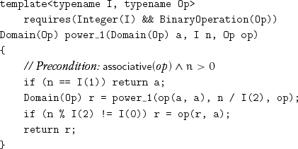
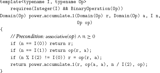
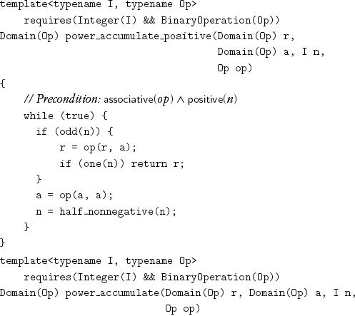
Our goal is to eliminate the recursive call. A first step is to transform the procedure to tail-recursive form, where the procedure’s execution ends with the recursive call. One of the techniques that allows this transformation is accumulation-variable introduction, where the accumulation variable carries the accumulated result between recursive calls:
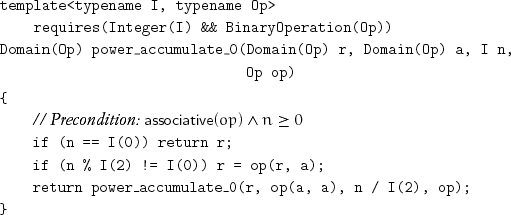
If r0, a0, and n0 are the original values of r, a, and n, this invariant holds at every recursive call: ![]() . As an additional benefit, this version computes not just power but also power multiplied by a coefficient. It also handles zero as the value of the exponent. However, power_accumulate_0 does an unnecessary squaring when going from 1 to 0. That can be eliminated by adding an extra case:
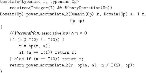
. As an additional benefit, this version computes not just power but also power multiplied by a coefficient. It also handles zero as the value of the exponent. However, power_accumulate_0 does an unnecessary squaring when going from 1 to 0. That can be eliminated by adding an extra case:
Adding the extra case results in a duplicated subexpression and in three tests that are not independent. Analyzing the dependencies between the tests and ordering the tests based on expected frequency gives
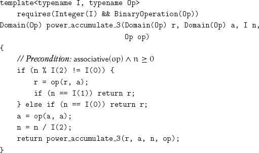
A strict tail-recursive procedure is one in which all the tail-recursive calls are done with the formal parameters of the procedure being the corresponding arguments:
A strict tail-recursive procedure can be transformed to an iterative procedure by replacing each recursive call with a goto to the beginning of the procedure or by using an equivalent iterative construct:

The recursion invariant becomes the loop invariant.
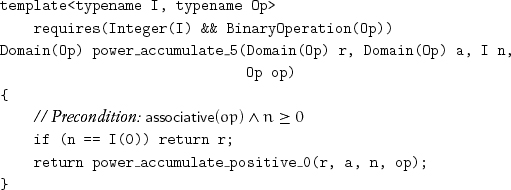
If n > 0 initially, it would pass through 1 before becoming 0. We take advantage of this by eliminating the test for 0 and strengthening the precondition:
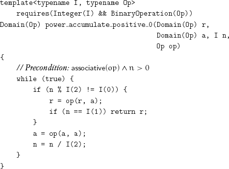
This is useful when it is known that n > 0. While developing a component, we often discover new interfaces.
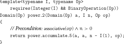
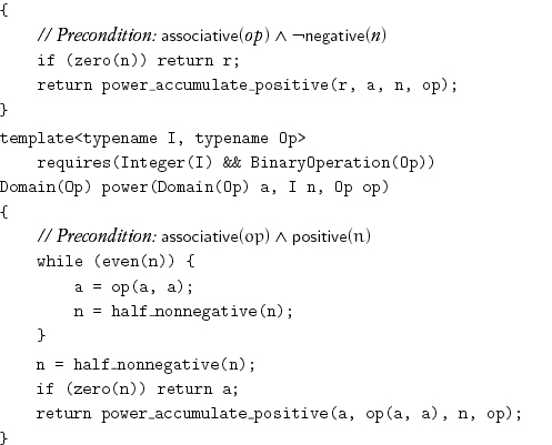
Now we relax the precondition again:
We can implement power from power_accumulate by using a simple identity:
an = aan–1
The transformation is accumulation-variable elimination:
This algorithm performs more operations than necessary. For example, when n is 16, it performs seven operations where only four are needed. When n is odd, this algorithm is fine. Therefore we can avoid the problem by repeated squaring of a and halving the exponent until it becomes odd:
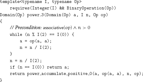
Exercise 3.1 Convince yourself that the last three lines of code are correct.
3.4 Special-Case Procedures
In the final versions we used these operations:
n / I(2)
n % I(2) == I(0)
n % I(2) != I(0)
n == I(0)
n == I(1)
Both / and % are expensive. We can use shifts and masks on non-negative values of both signed and unsigned integers.
It is frequently useful to identify commonly occuring expressions involving procedures and constants of a type by defining special-case procedures. Often these special cases can be implemented more efficiently than the general case and, therefore, belong to the computational basis of the type. For built-in types, there may exist machine instructions for the special cases. For user-defined types, there are often even more significant opportunities for optimizing special cases. For example, division of two arbitrary polynomials is more difficult than division of a polynomial by x. Similarly, division of two Gaussian integers (numbers of the form a + bi where a and b are integers and ![]() ) is more difficult than division of a Gaussian integer by 1 + i.
) is more difficult than division of a Gaussian integer by 1 + i.
Any integer type must provide the following special-case procedures:
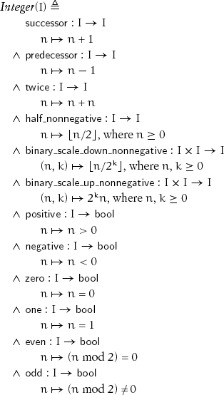
Exercise 3.2 Implement these procedures for C++ integral types.
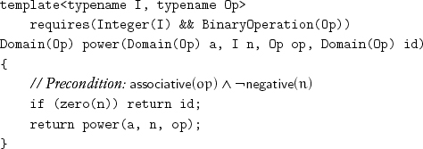
Now we can give the final implementations of the power procedures by using the special-case procedures:
Since we know that an+m = anam, a0 must evaluate to the identity element for the operation op. We can extend power to zero exponents by passing the identity element as another parameter:[6]
Project 3.1 Floating-point multiplication and addition are not associative, so they may give different results when they are used as the operation for power and power_left_associated; establish whether power or power_left_associated gives a more accurate result for raising a floating-point number to an integral power.
3.5 Parameterizing Algorithms
In power we use two different techniques for providing operations for the abstract algorithm.
1. The associative operation is passed as a parameter. This allows power to be used with different operations on the same type, such as multiplication modulo n.
2. The operations on the exponent are provided as part of the computational basis for the exponent type. We do not choose, for example, to pass half_nonnegative as a parameter to power, because we do not know of a case in which there are competing implementations of half_nonnegative on the same type.
In general, we pass an operation as a parameter when an algorithm could be used with different operations on the same type. When a procedure is defined with an operation as a parameter, a suitable default should be specified whenever possible. For example, the natural default for the operation passed to power is multiplication.
Using an operator symbol or a procedure name with the same semantics on different types is called overloading, and we say that the operator symbol or procedure name is overloaded on the type. For example, + is used on natural numbers, integers, rationals, polynomials, and matrices. In mathematics + is always used for an associative and commutative operation, so using + for string concatenation would be inconsistent. Similarly, when both + and × are present, × must distribute over +. In power, half_nonnegative is overloaded on the exponent type.
When we instantiate an abstract procedure, such as collision_point or power, we create overloaded procedures. When actual type parameters satisfy the requirements, the instances of the abstract procedure have the same semantics.
3.6 Linear Recurrences
A linear recurrence function of order k is a function f such that
![]()
where coefficients a0, ak–1 ≠ 0. A sequence {x0, x1, ...} is a linear recurrence sequence of order k if there is a linear recurrence function of order k—say, f—and
(∀n ≥ k)xn = f(xn–1, ..., xn–k)
Note that indices of x decrease. Given k initial values x0, ..., xk–1 and a linear recurrence function of order k, we can generate a linear recurrence sequence via a straightforward iterative algorithm. This algorithm requires n – k + 1 applications of the function to compute xn, for n ≥ k. As we will see, we can compute xn in O(log2n) steps, using power.[7] If ![]() is a linear recurrence function of order k, we can view f as performing vector inner product:[8]
is a linear recurrence function of order k, we can view f as performing vector inner product:[8]
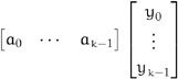
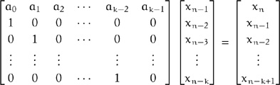
If we extend the vector of coefficients to the companion matrix with 1s on its subdiagonal, we can simultaneously compute the new value xn and shift the old values xn–1, ..., xn–k+1 to the correct positions for the next iteration:
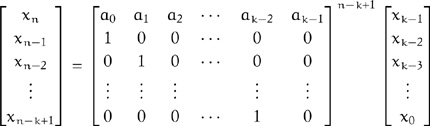
By the associativity of matrix multiplication, it follows that we can obtain xn by multiplying the vector of the k initial values by the companion matrix raised to the power n – k + 1:
Using power allows us to find xn with at most 2log2(n – k + 1) matrix multiplication operations. A straightforward matrix multiplication algorithm requires k3 multiplications and k3 – k2 additions of coefficients. Therefore the computation of xn requires no more than 2k3log2(n–k+1) multiplications and 2(k3–k2)log2(n–k+1) additions of the coefficients. Recall that k is the order of the linear recurrence and is a constant.[9]
We never defined the domain of the elements of a linear recurrence sequence. It could be integers, rationals, reals, or complex numbers: The only requirements are the existence of associative and commutative addition, associative multiplication, and distributivity of multiplication over addition.[10]
The sequence fi generated by the linear recurrence function
fib(y0, y1) = y0 + y1
of order 2 with initial values f0 = 0 and f1 = 1 is called the Fibonacci sequence.[11] It is straightforward to compute the nth Fibonacci number fn by using power with 2 × 2 matrix multiplication. We use the Fibonacci sequence to illustrate how the k3 multiplications can be reduced for this particular case. Let
![]()
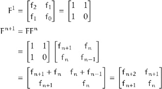
be the companion matrix for the linear recurrence generating the Fibonacci sequence. We can show by induction that
![]()
Indeed:
This allows us to express the matrix product of Fm and Fn as
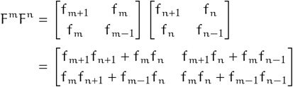
We can represent the matrix Fn with a pair corresponding to its bottom row, (fn, fn–1), since the top row could be computed as (fn–1 + fn, fn), which leads to the following code:
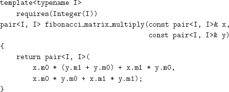
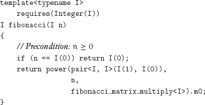
This procedure performs only four multiplications instead of the eight required for general 2 × 2 matrix multiplication. Since the first element of the bottom row of Fn is fn, the following procedure computes fn:
3.7 Accumulation Procedures
The previous chapter defined an action as a dual to a transformation. There is a dual procedure for a binary operation when it is used in a statement like
x = op(x, y);
Changing the state of an object by combining it with another object via a binary operation defines an accumulation procedure on the object. An accumulation procedure is definable in terms of a binary operation, and vice versa:
void op_accumulate(T& x, const T& y){x= op(x, y); }
// accumulation procedure from binary operation
and
T op(T x, const T& y) { op_accumulate(x, y); return x; }
// binary operation from accumulation procedure
As with actions, sometimes independent implementations are more efficient, in which case both operation and accumulation procedures need to be provided.
Exercise 3.3 Rewrite all the algorithms in this chapter in terms of accumulation procedures.
Project 3.2 Create a library for the generation of linear recurrence sequences based on the results of Miller and Brown [1966] and Fiduccia [1985].
3.8 Conclusions
Algorithms are abstract when they can be used with different models satisfying the same requirements, such as associativity. Code optimization depends on equational reasoning; unless types are known to be regular, few optimizations can be performed. Special-case procedures can make code more efficient and even more abstract. The combination of mathematics and abstract algorithms leads to surprising algorithms, such as logarithmic time generation of the nth element of a linear recurrence.