
Chapter 11
Partition and Merging
This chapter constructs predicate-based and ordering-based rearrangements from components from previous chapters. After presenting partition algorithms for forward and bidirectional iterators, we implement a stable partition algorithm. We then introduce a binary counter mechanism for transforming bottom-up divide-and-conquer algorithms, such as stable partition, into iterative form. We introduce a stable memory-adaptive merge algorithm and use it to construct an efficient memory-adaptive stable sort that works for forward iterators: the weakest concept that allows rearrangements.
11.1 Partition
In Chapter 6 we introduced the notion of a range partitioned by a predicate together with the fundamental algorithm partition_point on such a range. Now we look at algorithms for converting an arbitrary range into a partitioned range.
Exercise 11.1 Implement an algorithm partitioned_at_point that checks whether a given bounded range is partitioned at a specified iterator.
Exercise 11.2 Implement an algorithm potential_partition_point returning the iterator where the partition point would occur after partitioning.
Lemma 11.1 If m = potential_partition_point(f, l, p), then
count_if(f, m, p) = count_if_not(m, l, p)
In other words, the number of misplaced elements on either side of m is the same.
The lemma gives the minimum number of assignments to partition a range, 2n + 1, where n is the number of misplaced elements on either side of m: 2n assignments to misplaced elements and one assignment to a temporary variable.
Lemma 11.2 There are u!v! permutations that partition a range with u false values and v true values.
A partition rearrangement is stable if the relative order of the elements not satisfying the predicate is preserved, as is the relative order of the elements satisfying the predicate.
Lemma 11.3 The result of stable partition is unique.
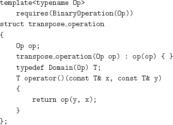
A partition rearrangement is semistable if the relative order of elements not satisfying the predicate is preserved. The following algorithm performs a semistable partition:[1]
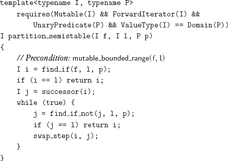
The correctness of partition_semistable depends on the following three lemmas.
Lemma 11.4 Before the exit test, none(f, i, p) ![]() all(i, j, p).
all(i, j, p).
Lemma 11.5 After the exit test, p(source(i)) ![]() ¬p(source(j)).
¬p(source(j)).
Lemma 11.6 After the call of swap_step, none(f, i, p) ![]() all(i, j, p).
all(i, j, p).
Semistability follows from the fact that the swap_step call moves an element not satisfying the predicate before a range of elements satisfying the predicate, and therefore the order of elements not satisfying the predicate does not change.
partition_semistable uses only one temporary object, in swap_step.
Let n = l – f be the number of elements in the range, and let w be the number of elements not satisfying the predicate that follow the first element satisfying the predicate. Then the predicate is applied n times, exchange_values is performed w times, and the number of iterator increments is n + w.
Exercise 11.3 Rewrite partition_semistable, expanding the call of find_if_not inline and eliminating the extra test against l.
Exercise 11.4 Give the postcondition of the algorithm that results from replacing swap_step(i, j) with copy_step(j, i)in partition_semistable, suggest an appropriate name, and compare its use with the use of partition_semistable.
Let n be the number of elements in a range to be partitioned.
Lemma 11.7 A partition rearrangement that returns the partition point requires n applications of the predicate.
Lemma 11.8 A partition rearrangement of a nonempty range that does not return the partition point requires n – 1 applications of the predicate.[2]
Exercise 11.5 Implement a partition rearrangement for nonempty ranges that performs n – 1 predicate applications.
Consider a range with one element satisfying the predicate, followed by n elements not satisfying the predicate. partition_semistable will perform n calls of exchange_values, while one suffices. If we combine a forward search for an element satisfying the predicate with a backward search for an element not satisfying the predicate, we avoid unnecessary exchanges. The algorithm requires bidirectional iterators:
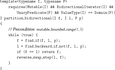
As with partition_semistable, partition_bidirectional uses only one temporary object.
Lemma 11.9 The number of times exchange_values is performed, v, equals the number of misplaced elements not satisfying the predicate. The total number of assignments, therefore, is 3v.
Exercise 11.6 Implement a partition rearrangement for forward iterators that calls exchange_values the same number of times as partition_bidirectional by first computing the potential partition point.
It is possible to accomplish partition with a different rearrangement that has only a single cycle, resulting in 2v + 1 assignments. The idea is to save the first misplaced element, creating a “hole,” then repeatedly find a misplaced element on the opposite side of the potential partition point and move it into the hole, creating a new hole, and finally move the saved element into the last hole.
Exercise 11.7 Using this technique, implement partition_single_cycle.
Exercise 11.8 Implement a partition rearrangement for bidirectional iterators that finds appropriate sentinel elements and then uses find_if_unguarded and an unguarded version of find_backward_if_not.
Exercise 11.9 Repeat the previous exercise, incorporating the single-cycle technique.
The idea for a bidirectional partition algorithm, as well as the single-cycle and sentinel variations, are from C. A. R. Hoare.[3]
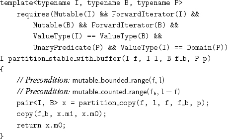
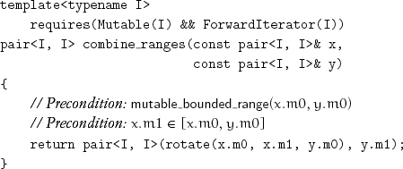
When stability is needed for both sides of the partition and enough memory is available for a buffer of the same size as the range, the following algorithm can be used:
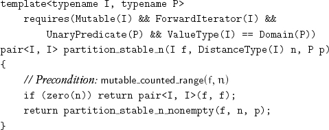
When there is not enough memory for a full-size buffer, it is possible to implement stable partition by using a divide-and-conquer algorithm. If the range is a singleton range, it is already partitioned, and its partition point can be determined with one predicate application:
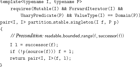
The returned value is the partition point and the limit of the range: in other words, the range of values satisfying the predicate.
Two adjacent partitioned ranges can be combined into a single partitioned range by rotating the range bounded by the first and second partition points around the middle:
Lemma 11.10 combine_ranges is associative when applied to three nonoverlapping ranges.
Lemma 11.11 If, for some predicate p,
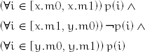
then after
z ← combine_ranges(x, y)
the following hold:
![]()
The inputs are the ranges of values satisfying the predicate and so is the output; therefore a nonsingleton range is stably partitioned by dividing it in the middle, partitioning both halves recursively, and then combining the partitioned parts:
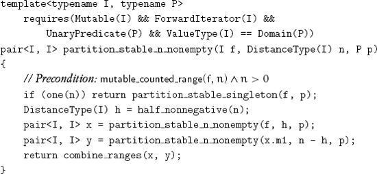
Since empty ranges never result from subdividing a range of size greater than 1, we handle that case only at the top level:
Exactly n predicate applications are performed at the bottom level of recursion. The depth of the recursion for partition_stable_n_nonempty is ![]() log2n
log2n![]() . At every recursive level, we rotate n/2 elements on the average, requiring between n/2 and 3n/2 assignments, depending on the iterator category. The total number of assignments is nlog2n/2 for random-access iterators and 3nlog2n/2 for forward and bidirectional iterators.
. At every recursive level, we rotate n/2 elements on the average, requiring between n/2 and 3n/2 assignments, depending on the iterator category. The total number of assignments is nlog2n/2 for random-access iterators and 3nlog2n/2 for forward and bidirectional iterators.
Exercise 11.10 Use techniques from the previous chapter to produce a memory-adaptive version of partition_stable_n.
11.2 Balanced Reduction
Although the performance of partition_stable_n depends on subdividing the range in the middle, its correctness does not. Since combine_ranges is a partially associative operation, the subdivision could be performed at any point. We can take advantage of this fact to produce an iterative algorithm with similar performance; such an algorithm is useful, for example, when the size of the range is not known in advance or to eliminate procedure call overhead. The basic idea is to use reduction, applying partition_stable_singleton to each singleton range and combining the results with combine_ranges:
reduce_nonempty(
f, l,
combine_ranges<I>,
partition_trivial<I, P>(p));
where partition_trivial is a function object that binds the predicate parameter to partition_stable_singleton:
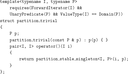
Using reduce_nonempty leads to quadratic complexity. We need to take advantage of partial associativity to create a balanced reduction tree. We use a binary counter technique to build the reduction tree bottom-up.[4] A hardware binary counter increments an n-bit binary integer by 1. A 1 in position i has a weight of 2i; a carry from this position has a weight of 2i+1 and propagates to the next-higher position. Our counter uses the “bit” in position i to represent either empty or the result of reducing 2i elements from the original range. When the carry propagates to the next higher position, it is either stored or is combined with another value of the same weight. The carry from the highest position is returned by the following procedure, which takes the identity element as an explicit parameter, as does reduce_nonzeroes:
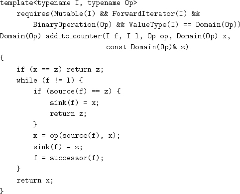
Storage for the counter is provided by the following type, which handles over-flows from add_to_counter by extending the counter:
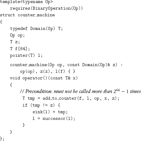
This uses a built-in C++ array; alternative implementations are possible.[5]
After add_to_counter has been called for every element of a range, the nonempty positions in the counter are combined with leftmost reduction to produce the final result:
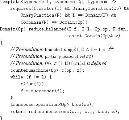
The values in higher positions of the counter correspond to earlier elements of the original range, and the operation is not necessarily commutative. Therefore we must use a transposed version of the operation, which we obtain by using the following function object:
Now we can implement an iterative version of stable partition with the following procedure:
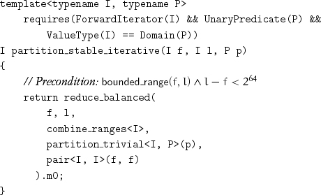
pairI, I(f, f) is a good way to represent the identity element since it is never returned by partition_trivial or the combining operation.
The iterative algorithm constructs a different reduction tree than the recursive algorithm. When the size of the problem is equal to 2k, the recursive and iterative versions perform the same sequence of combining operations; otherwise the iterative version may do up to a linear amount of extra work. For example, in some algorithms the complexity goes from nlog2n to nlog2![]() .
.
Exercise 11.11 Implement an iterative version of sort_linked_nonempty_n from Chapter 8, using reduce_balanced.
Exercise 11.12 Implement an iterative version of reverse_n_adaptive from Chapter 10, using reduce_balanced.
Exercise 11.13 Use reduce_balanced to implement an iterative and memory-adaptive version of partition_stable_n.
11.3 Merging
In Chapter 9 we presented copying merge algorithms that combine two increasing ranges into a third increasing range. For sorting, it is useful to have a rearrangement that merges two adjacent increasing ranges into a single increasing range. With a buffer of size equal to that of the first range, we can use the following procedure:[6]
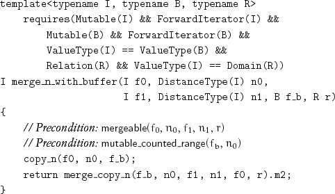
where mergeable is defined as follows:
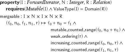
Lemma 11.12 The postcondition for merge_n_with_buffer is
increasing_counted_range(f0, n0 + n1, r)
A merge is stable if the output range preserves the relative order of equivalent elements both within each input range and between the first and second input range.
Lemma 11.13 merge_n_with_buffer is stable.
Note that merge_linked_nonempty, merge_copy, and merge_copy_backward are also stable.
We can sort a range with a buffer of half of its size:[7]
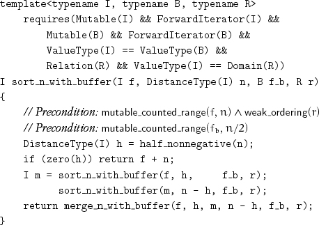
Lemma 11.14 The postcondition for sort_n_with_buffer is
increasing_counted_range(f, n, r)
A sorting algorithm is stable if it preserves the relative order of elements with equivalent values.
Lemma 11.15 sort_n_with_buffer is stable.
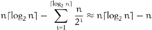
The algorithm has ![]() log2n
log2n![]() recursive levels. Each level performs at most 3n/2 assignments, for a total bounded by
recursive levels. Each level performs at most 3n/2 assignments, for a total bounded by ![]() . At the ith level from the bottom, the worst-case number of comparisons is
. At the ith level from the bottom, the worst-case number of comparisons is ![]() , giving us the following bound on the number of comparisons:
, giving us the following bound on the number of comparisons:
When a buffer of sufficient size is available, sort_n_with_buffer is an efficient algorithm. When less memory is available, a memory-adaptive merge algorithm can be used. Subdividing the first subrange in the middle and using the middle element to subdivide the second subrange at its lower bound point results in four subranges r0, r1, r2, and r3 such that the values in r2 are strictly less than the values in r1. Rotating the ranges r2 and r3 leads to two new merge subproblems (r0 with r2 and r1 with r3):
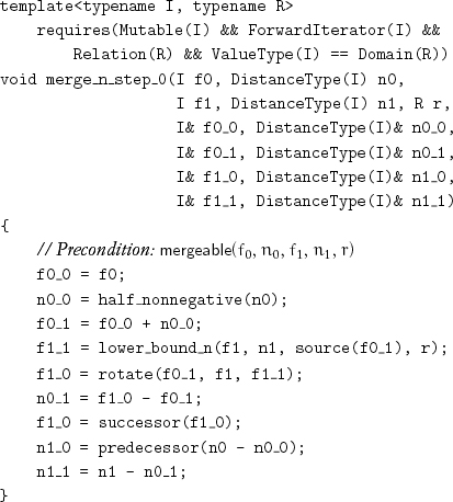
Lemma 11.16 The rotate does not change the relative positions of elements with equivalent values.
An iterator i in a range is a pivot if its value is not smaller than any value preceding it and not larger than any value following it.
Lemma 11.17 After merge_n_step_0, f1_0 is a pivot.
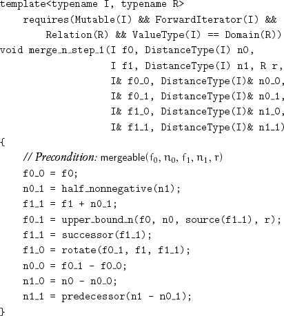
We can perform an analogous subdivision from the right by using upper_bound:
This leads to the following algorithm from Dudzi![]() ski and Dydek [1981]:
ski and Dydek [1981]:
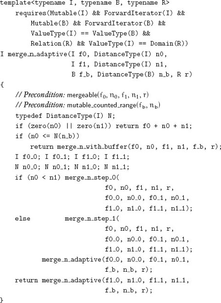
Lemma 11.18 merge_n_adaptive terminates with an increasing range.
Lemma 11.19 merge_n_adaptive is stable.
Lemma 11.20 There are at most ![]() log2(min(n0, n1))
log2(min(n0, n1))![]() + 1 recursive levels.
+ 1 recursive levels.
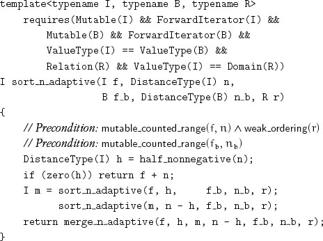
Using merge_n_adaptive, we can implement the following sorting procedure:
Exercise 11.14 Determine formulas for the number of assignments and the number of comparisons as functions of the size of the input and buffer ranges. Dudzi![]() ski and Dydek [1981] contains a careful complexity analysis of the case in which there is no buffer.
ski and Dydek [1981] contains a careful complexity analysis of the case in which there is no buffer.
We conclude with the following algorithm:
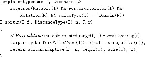
It works on ranges with minimal iterator requirements, is stable, and is efficient even when temporary_buffer is only able to allocate a few percent of the requested memory.
Project 11.1 Develop a library of sorting algorithms constructed from abstract components. Design a benchmark to analyze their performance for different array sizes, element sizes, and buffer sizes. Document the library with recommendations for the circumstances in which each algorithm is appropriate.
11.4 Conclusions
Complex algorithms are decomposable into simpler abstract components with carefully defined interfaces. The components so discovered are then used to implement other algorithms. The iterative process going from complex to simple and back is central to the discovery of a systematic catalog of efficient components.