Chapter 10

Rearrangements

This chapter introduces the concept of permutation and a taxonomy for a class of algorithms, called rearrangements, that permute the elements of a range to satisfy a given postcondition. We provide iterative algorithms of reverse for bidirectional and random-access iterators, and a divide-and-conquer algorithm for reverse on forward iterators. We show how to transform divide-and-conquer algorithms to make them run faster when extra memory is available. We describe three rotation algorithms corresponding to different iterator concepts, where rotation is the interchange of two adjacent ranges of not necessarily equal size. We conclude with a discussion of how to package algorithms for compile-time selection based on their requirements.

10.1 Permutations

A transformation f is an into transformation if, for all x in its definition space, there exists a y in its definition space such that y = f(x). A transformation f is an onto transformation if, for all y in its definition space, there exists an x in its definition space such that y = f(x). A transformation f is a one-to-one transformation if, for all x, x′ in its definition space, f(x) = f(x′) x = x′.

Lemma 10.1 A transformation on a finite definition space is an onto transformation if and only if it is both an into and one-to-one transformation.

Exercise 10.1 Find a transformation of the natural numbers that is both an into and onto transformation but not a one-to-one transformation, and one that is both an into and one-to-one transformation but not an onto transformation.

A fixed point of a transformation is an element x such that f(x) = x. An identity transformation is one that has every element of its definition space as a fixed point. We denote the identity transformation on a set S as identity_S.

A permutation is an onto transformation on a finite definition space. An example of a permutation on [0, 6):

p (0) = 5
p (1) = 2
p (2) = 4
p (3) = 3
p (4) = 1
p (5) = 0

If p and q are two permutations on a set S, the composition q p takes x S to q(p(x)).

Lemma 10.2 The composition of permutations is a permutation.

Lemma 10.3 Composition of permutations is associative.

Lemma 10.4 For every permutation p on a set S, there is an inverse permutation p^–1 such that p^–1 p = p p^–1 = identity_S.

The permutations on a set form a group under composition.

Lemma 10.5 Every finite group is a subgroup of a permutation group of its elements, where every permutation in the subgroup is generated by multiplying all the elements by an individual element.

For example, the multiplication group modulo 5 has the following multiplication table:

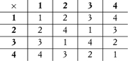
Every row and column of the multiplication table is a permutation. Since not every one of the 4! = 24 permutations of four elements appears in it, the multiplication group modulo 5 is therefore a proper subgroup of the permutation group of four elements.

A cycle is a circular orbit within a permutation. A trivial cycle is one with a cycle size of 1; the element in a trivial cycle is a fixed point. A permutation containing a single nontrivial cycle is called a cyclic permutation. A transposition is a cyclic permutation with a cycle size of 2.

Lemma 10.6 Every element in a permutation belongs to a unique cycle.

Lemma 10.7 Any permutation of a set with n elements contains k ≤ n cycles.

Lemma 10.8 Disjoint cyclic permutations commute.

Exercise 10.2 Show an example of two nondisjoint cyclic permutations that do not commute.

Lemma 10.9 Every permutation can be represented as a product of the cyclic permutations corresponding to its cycles.

Lemma 10.10 The inverse of a permutation is the product of the inverses of its cycles.

Lemma 10.11 Every cyclic permutation is a product of transpositions.

Lemma 10.12 Every permutation is a product of transpositions.

A finite set S of size n is a set for which there exists a pair of functions

choose_S : [0, n) → S
 index_S : S → [0, n)

satisfying

choose_S(index_S(x)) = x
index_S(choose_S(i)) = i

In other words, S can be put into one-to-one correspondence with a range of natural numbers.

If p is a permutation on a finite set S of size n, there is a corresponding index permutation p′ on [0, n) defined as

p′(i) = index_S(p(choose_S(i)))

Lemma 10.13 p(x) = choose_S(p′(index_S(x)))

We will frequently define permutations by the corresponding index permutations.

10.2 Rearrangements

A rearrangement is an algorithm that copies the objects from an input range to an output range such that the mapping between the indices of the input and output ranges is a permutation. This chapter deals with position-based rearrangements, where the destination of a value depends only on its original position and not on the value itself. The next chapter deals with predicate-based rearrangements, where the destination of a value depends only on the result of applying a predicate to a value, and ordering-based rearrangements, where the destination of a value depends only on the ordering of values.

In Chapter 8 we studied link rearrangements, such as reverse linked, where links are modified to establish a rearrangement. In Chapter 9 we studied copying rearrangements, such as copy and reverse_copy. In this and the next chapter we study mutative rearrangements, where the input and output ranges are identical.

Every mutative rearrangement corresponds to two permutations: a to-permutation mapping an iterator i to the iterator pointing to the destination of the element at i and a from-permutation mapping an iterator i to the iterator pointing to the origin of the element moved to i.

Lemma 10.14 The to-permutation and from-permutation for a rearrangement are inverses of each other.

If the to-permutation is known, we can rearrange a cycle with this algorithm:

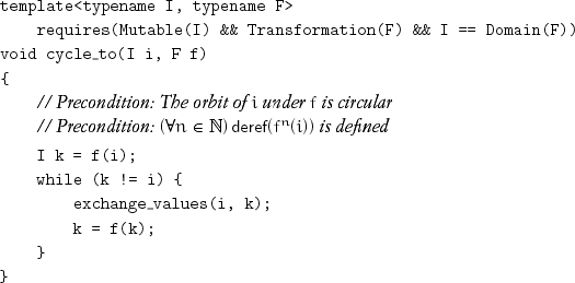
After cycle_to(i, f), the value of source(f(j)) and the original value of source(j) are equal for all j in the orbit of i under f. The call performs 3(n – 1) assignments for a cycle of size n.

Exercise 10.3 Implement a version of cycle_to that performs 2n – 1 assignments.

If the from-permutation is known, we can rearrange a cycle with this algorithm:

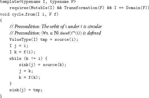
After cycle_from (i, f), the value of source(j) and the original value of source(f(j)) are equal for all j in the orbit of i under f. The call performs n + 1 assignments, whereas implementing it with exchange_values would perform 3(n – 1) assignments. Observe that we require only mutability on the type I; we do not need any traversal functions, because the transformation f performs the traversal. In addition to the from-permutation, implementing a mutative rearrangement using cycle_from requires a way to obtain a representative element from each cycle. In some cases the cycle structure and representatives of the cycles are known.

Exercise 10.4 Implement an algorithm that performs an arbitrary rearrangement of a range of indexed iterators. Use an array of n Boolean values to mark elements as they are placed, and scan this array for an unmarked value to determine a representive of the next cycle.

Exercise 10.5 Assuming iterators with total ordering, design an algorithm that uses constant storage to determine whether an iterator is a representative for a cycle; use this algorithm to implement an arbitrary rearrangement.

Lemma 10.15 Given a from-permutation, it is possible to perform a mutative rearrangement using n + c_N – c_T assignments, where n is the number of elements, c_N the number of nontrivial cycles, and c_T the number of trivial cycles.

10.3 Reverse Algorithms

A simple but useful position-based mutative rearrangement is reversing a range. This rearrangement is induced by the reverse permutation on a finite set with n elements, which is defined by the index permutation

p(i) = (n – 1) – i

Lemma 10.16 The number of nontrivial cycles in a reverse permutation is n/2; the number of trivial cycles is n mod 2.

Lemma 10.17 n/2 is the largest possible number of nontrivial cycles in a permutation.

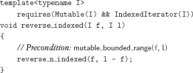
The definition of reverse directly gives the following algorithm for indexed iterators:^[1]

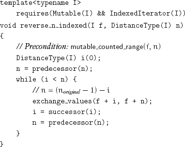
If the algorithm is used with forward or bidirectional iterators, it performs a quadratic number of iterator increments. For bidirectional iterators, two tests per iteration are required:

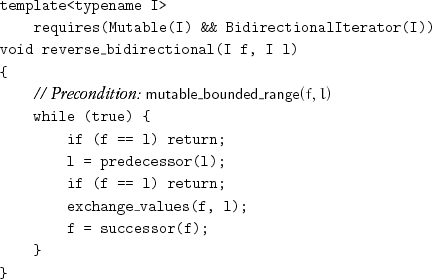
When the size of the range is known, reverse_swap_ranges_n can be used:

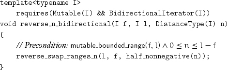
The order of the first two arguments to reverse_swap_ranges_n is determined by the fact that it moves backward in the first range. Passing n < l – f to reverse_n_bidirectional leaves values in the middle in their original positions.

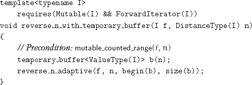
When a data structure provides forward iterators, they are sometimes linked iterators, in which case reverse_linked can be used. In other cases extra buffer memory may be available, allowing the following algorithm to be used:

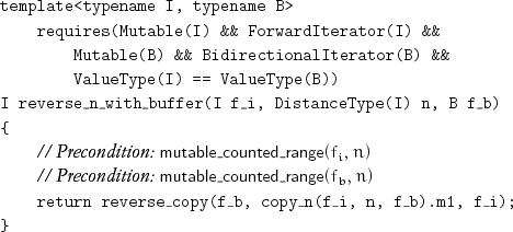
reverse_n_with_buffer performs 2n assignments.

We will use this approach of copying to a buffer and back for other rearrangements.

If no buffer memory is available but logarithmic storage is available as stack space, a divide-and-conquer algorithm is possible: Split the range into two parts, reverse each part, and, finally, interchange the parts with swap_ranges_n.

Lemma 10.18 Splitting as evenly as possible minimizes the work.

Returning the limit allows us to optimize traversal to the midpoint by using the technique we call auxiliary computation during recursion:

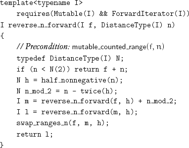
The correctness of reverse_n_forward depends on the following.

Lemma 10.19 The reverse permutation on [0, n) is the only permutation satisfying i < j p(j) < p(i).

This condition obviously holds for ranges of size 1. The recursive calls inductively establish that the condition holds within each half. The condition between the halves and the skipped middle element, if any, is reestablished with swap_ranges_n.

Lemma 10.20 For a range of length , where a_i is the ith digit in the binary representation of n, the number of assignments is .

reverse_n_forward requires a logarithmic amount of space for the call stack. A memory-adaptive algorithm uses as much additional space as it can acquire to maximize performance. A few percent of additional space gives a large performance improvement. That leads to the following algorithm, which uses divide and conquer and switches to the linear-time reverse_n_with_buffer whenever the subproblem fits into the buffer:

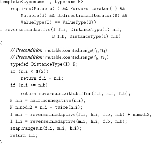
Exercise 10.6 Derive a formula for the number of assignments performed by reverse_n_adaptive for given range and buffer sizes.

10.4 Rotate Algorithms

The permutation p of n elements defined by an index permutation p(i) = (i + k) mod n is called the k-rotation.

Lemma 10.21 The inverse of a k-rotation of n elements is an (n – k)-rotation.

An element with index i is in the cycle

{i, (i + k) mod n, (i + 2k) mod n, ... } = {(i + uk) mod n}

The length of the cycle is the smallest positive integer m such that

i = (i + mk) mod n

This is equivalent to mk mod n = 0, which shows the length of the cycle to be independent of i. Since m is the smallest positive number such that mk mod n = 0, lcm(k, n) = mk, where lcm(a, b) is the least common multiple of a and b. Using the standard identity

lcm(a, b) gcd(a, b) = ab

we obtain that the size of the cycle

The number of cycles, therefore, is gcd(k, n).

Consider two elements in a cycle: (i + uk) mod n and (i + vk) mod n. The distance between them is

|(i + uk) mod n – (i + vk) mod n| = (u – v)k mod n
                                  = (u – v)k – pn

where p = quotient((u – v)k, n). Since both k and n are divisible by d = gcd(k, n), so is the distance. Therefore the distance between different elements in the same cycle is at least d, and elements with indices in [0, d) belong to disjoint cycles.

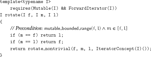
k-rotation rearrangement of a range [f, l) is equivalent to interchanging the relative positions of the values in the subranges [f, m) and [m, l), where m = f + ((l – f) – k) = l – k. m is a more useful input than k. When forward or bidirectional iterators are involved, it avoids performing linear-time operations to compute m from k. Returning the iterator m′ = f + k pointing to the new position of the element at f is useful for many other algorithms.^[2]

Lemma 10.22 Rotating a range [f, l) around the iterator m and then rotating it around the returned value m returns m and restores the range to its original state.

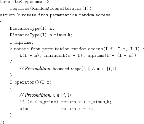
We can use cycle_from to implement a k-rotation rearrangement of a range of indexed or random-access iterators. The to-permutation is p(i) = (i+k) mod n, and the from-permutation is its inverse: p^–1(i) = (i+(n–k)) mod n, where n–k = m–f. We want to avoid evaluating mod, and we observe that

That leads to the following function object for random-access iterators:

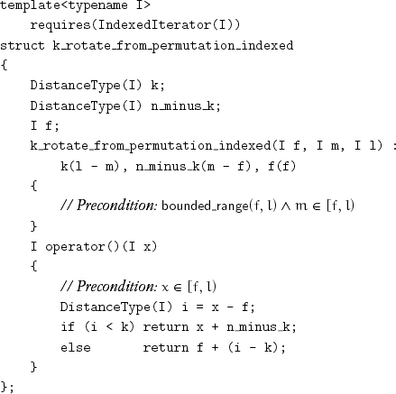
For indexed iterators, the absence of natural ordering and subtraction of a distance from an iterator costs an extra addition or two:

This procedure rotates every cycle:

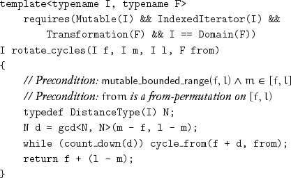
This algorithm was first published in Fletcher and Silver [1966] except that they used cycle_to where we use cycle_from. These procedures select the appropriate function object:

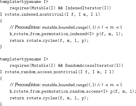
The number of assignments is n + c_N – c_T = n + gcd(n, k). Recall that n is the number of elements, c_N the number of nontrivial cycles, and c_T the number of trivial cycles. The expected value of gcd(n, k) for 1 ≤ n, k ≤ m is ln m + C + (see Diaconis and Erd ös [2004]).

The following property leads to a rotation algorithm for bidirectional iterators.

Lemma 10.23 The k-rotation on [0, n) is the only permutation p that inverts the relative ordering between the subranges [0, n–k) and [n–k, n) but preserves the relative ordering within each subrange:

1. i < n – k  n – k ≤ j < n  p(j) < p(i)
2. i < j < n – k  n – k ≤ i < j  p(i) < p(j)

The reverse rearrangement satisfies condition 1 but not 2. Applying reverse to subranges [0, n – k) and [n – k, n) and then applying reverse to the entire range will satisfy both conditions:

   reverse_bidirectional(f, m);
   reverse_bidirectional(m, l);
   reverse_bidirectional(f, l);

Finding the return value m′ is handled by using reverse_swap_ranges_bounded:^[3]

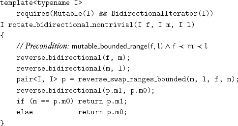
Lemma 10.24 The number of assignments is 3(n/2 + k/2 + (n–k)/2), which is 3n when both n and k are even and 3(n–2) otherwise.

Given a range [f, l) and an iterator m in that range, a call

p ← swap_ranges_bounded(f, m, m, l)

sets p to a pair of iterators such that

p.m0 = m  p.m1 = l

If p.m0 = m p.m0 = l, we are done. Otherwise [f, p.m0) are in the final position and, depending on whether p.m0 = m or p.m1 = l, we need to rotate [p.m0, l) around p.m1 or m, respectively. This immediately leads to the following algorithm, first published in Gries and Mills [1981]:

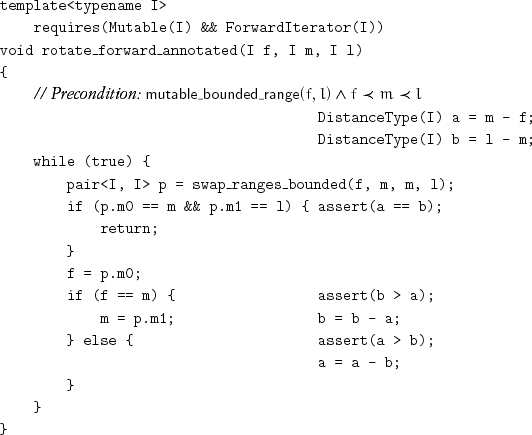
Lemma 10.25 The first time the else clause is taken, f = m′, the standard return value for rotate.

The annotation variables a and b remain equal to the sizes of the two subranges to be swapped. At the same time, they perform subtractive gcd of the initial sizes. Each call of exchange_values performed by swap_ranges_bounded puts one value into its final position, except during the final call of swap_ranges_bounded, when each call of exchange_values puts two values into their final positions. Since the final call of swap_ranges_bounded performs gcd(n, k) calls of exchange_values, the total number of calls to exchange_values is n – gcd(n, k).

The previous lemma suggests one way to implement a complete rotate_forward: Create a second copy of the code that saves a copy of f in the else clause and then invokes rotate_forward_annotated to complete the rotation. This can be transformed into the following two procedures:

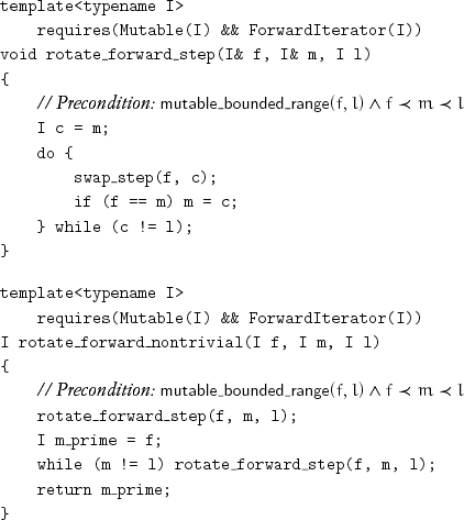
Exercise 10.7 Verify that rotate_forward_nontrivial rotates [f, l) around m and returns m′.

Sometimes, it is useful to partially rotate a range, moving the correct objects to [f, m′) but leaving the objects in [m′, l) in some rearrangement of the objects originally in [f, m). For example, this can be used to move undesired objects to the end of a sequence in preparation for erasing them. We can accomplish this with the following algorithm:

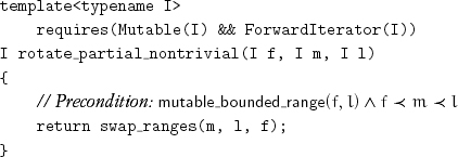
Lemma 10.26 The postcondition for rotate_partial_nontrivial is that it performs a partial rotation such that the objects in positions [m′, l) are k-rotated where k = – (l – f) mod (m – f).

A backward version of rotate_partial_nontrivial that uses a backward version of swap_ranges could be useful sometimes.

When extra buffer memory is available, the following algorithm may be used:

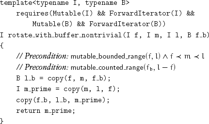
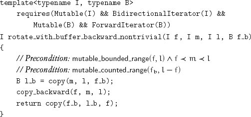
rotate_with_buffer_nontrivial performs (l – f)+(m – f) assignments, whereas the following algorithm performs (l–f)+(l–m) assignments. When rotating a range of bidirectional iterators, the algorithm minimizing the number of assignments could be chosen, although computing the differences at runtime requires a linear number of successor operations:

10.5 Algorithm Selection

In Section 10.3 we presented reverse algorithms with a variety of iterator requirements and procedure signatures, including versions taking counted and bounded ranges. It is worth defining variations that make the most convenient signatures available for additional iterator types. For example, an additional constant-time iterator difference leads to the algorithm for reversing a bounded range of indexed iterators:

When a range of forward iterators must be reversed, there is usually enough extra memory available to allow reverse_n_adaptive to run efficiently. When the size of the range to be reversed is moderate, it can be obtained in the usual way (for example, malloc). However, when the size is very large, there might not be enough available physical memory to allocate a buffer of this size. Because algorithms such as reverse_n_adaptive run efficiently even when the size of the buffer is small in proportion to the range being mutated, it is useful for the system to provide a way to allocate a temporary buffer. The allocation may reserve less memory than requested; in a system with virtual memory, the allocated memory has physical memory assigned to it. A temporary buffer is intended for short-term use and is guaranteed to be returned when the algorithm terminates.

For example, the following algorithm uses a type temporary_buffer:

The constructor b(n) allocates memory to hold some number m ≤ n adjacent objects of type ValueType(I); size(b) returns the number m, and begin(b) returns an iterator pointing to the beginning of this range. The destructor for b deallocates the memory.

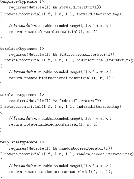
For the same problem, there are often different algorithms for different type requirements. For example, for rotate there are three useful algorithms for indexed (and random access), bidirectional, and forward iterators. It is possible to automatically select from a family of algorithms, based on the requirements the types satisfy. We accomplish this by using a mechanism known as concept dispatch. We start by defining a top-level dispatch procedure, which in this case also handles trivial rotates:

The type function IteratorConcept returns a concept tag type, a type that encodes the strongest concept modeled by its argument. We then implement a procedure for each concept tag type:

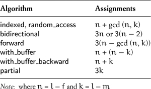
Concept dispatch does not take into consideration factors other than type requirements. For example, as summarized in Table 10.1, we can rotate a range of random-access iterators by using three algorithms, each performing a different number of assignments. When the range fits into cache memory, the n + gcd(n, k) assignments performed by the random-access algorithm give us the best performance. But when the range does not fit into cache, the 3n assignments of the bidirectional algorithm or the 3(n–gcd(n, k)) assignments of the forward algorithm are faster. In this case additional factors are affecting whether the bidirectional or forward algorithm will be fastest, including the more regular loop structure of the bidirectional algorithm, which can make up for the additional assignments it performs, and details of the processor architecture, such as its cache configuration and prefetch logic. It should also be noted that the algorithms perform iterator operations in addition to assignments of the value type; as the size of the value type gets smaller, the relative cost of these other operations increases.

Table 10.1. Number of Assignments Performed by Rotate Algorithms

Project 10.1 Design a benchmark comparing performance of all the algorithms for different array sizes, element sizes, and rotation amounts. Based on the results of the benchmark, design a composite algorithm that appropriately uses one of the rotate algorithms depending on the iterator concept, size of the range, amount of rotation, element size, cache size, availability of temporary buffer, and other relevant considerations.

Project 10.2 We have presented two kinds of position-based rearrangement algorithms: reverse and rotate. There are, however, other examples of such algorithms in the literature. Develop a taxonomy of position-based rearrangements, catalog existing algorithms, discover missing algorithms, and produce a library.

10.6 Conclusions

The structure of permutations allows us to design and analyze rearrangement algorithms. Even simple problems, such as reverse and rotate, lead to a variety of useful algorithms. Selecting the appropriate one depends on iterator requirements and system issues. Memory-adaptive algorithms provide a practical alternative to the theoretical notion of in-place algorithms.