Chapter 6
Iterators
This chapter introduces the concept of iterator: an interface between algorithms and sequential data structures. A hierarchy of iterator concepts corresponds to different kinds of sequential traversals: single-pass forward, multipass forward, bidirectional, and random access.[1] We investigate a variety of interfaces to common algorithms, such as linear and binary search. Bounded and counted ranges provide a flexible way of defining interfaces for variations of a sequential algorithm.
6.1 Readability
Every object has an address: an integer index into computer memory. Addresses allow us to access or modify an object. In addition, they allow us to create a wide variety of data structures, many of which rely on the fact that addresses are effectively integers and allow integer-like operations.
Iterators are a family of concepts that abstract different aspects of addresses, allowing us to write algorithms that work not only with addresses but also with any addresslike objects satisfying the minimal set of requirements. In Chapter 7 we introduce an even broader conceptual family: coordinate structures.
There are two kinds of operations on iterators: accessing values or traversal. There are three kinds of access: reading, writing, or both reading and writing. There are four kinds of linear traversal: single-pass forward (an input stream), multipass forward (a singly linked list), bidirectional (a doubly linked list), and random access (an array).
This chapter studies the first kind of access: readability, that is, the ability to obtain the value of the object denoted by another. A type T is readable if a unary function source defined on it returns an object of type ValueType (T):
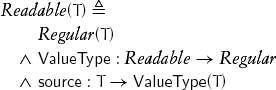
source is only used in contexts in which a value is needed; its result can be passed to a procedure by value or by constant reference.
There may be objects of a readable type on which source is not defined; source does not have to be total. The concept does not provide a definition-space predicate to determine whether source is defined for a particular object. For example, given a pointer to a type T, it is impossible to determine whether it points to a validly constructed object. Validity of the use of source in an algorithm must be derivable from preconditions.
Accessing data by calling source on an object of a readable type is as fast as any other way of accessing this data. In particular, for an object of a readable type with value type T residing in main memory, we expect the cost of source to be approximately equal to the cost of dereferencing an ordinary pointer to T. As with ordinary pointers, there could be nonuniformity owing to the memory hierarchy. In other words, there is no need to store pointers instead of iterators to speed up an algorithm.
It is useful to extend source to types whose objects don’t point to other objects. We do this by having source return its argument when applied to an object of such a type. This allows a program to specify its requirement for a value of type T in such a way that the requirement can be satisfied by a value of type T, a pointer to type T, or, in general, any readable type with a value type of T. Therefore we assume that unless otherwise defined, ValueType (T) = T and that source returns the object to which it is applied.
6.2 Iterators
Traversal requires the ability to generate new iterators. As we saw in Chapter 2, one way to generate new values of a type is with a transformation. While transformations are regular, some one-pass algorithms do not require regularity of traversal, and some models, such as input streams, do not provide regularity of traversal. Thus the weakest iterator concept requires only the pseudotransformation[2] successor and the type function DistanceType:
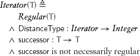
DistanceType returns an integer type large enough to measure any sequence of applications of successor allowable for the type. Since regularity is assumed by default, we must explicitly state that it is not a requirement for successor.
As with source on readable types, successor does not have to be total; there may be objects of an iterator type on which successor is not defined. The concept does not provide a definition-space predicate to determine whether successor is defined for a particular object. For example, a pointer into an array contains no information indicating how many times it could be incremented. Validity of the use of successor in an algorithm must be derivable from preconditions.
The following defines the action corresponding to successor:
template<typename I>
requires(Iterator(I))
void increment(I& x)
{
// Precondition: successor(x) is defined
x = successor(x);
}
Many important algorithms, such as linear search and copying, are single-pass; that is, they apply successor to the value of each iterator once. Therefore they can be used with input streams, and that is why we drop the requirement for successor to be regular: i = j does not imply successor(i) = successor(j) even when successor is defined. Furthermore, after successor(i) is called, i and any iterator equal to it may no longer be well formed. They remain partially formed and can be destroyed or assigned to; successor, source, and = should not be applied to them.
Note that successor(i) = successor(j) does not imply that i = j. Consider, for example, two null-terminating singly linked lists.
An iterator provides as fast a linear traversal through an entire collection of data as any other way of traversing that data.
In order for an integer type to model Iterator, it must have a distance type. An unsigned integer type is its own distance type; for any bounded signed binary integer type Sn, its distance type is the corresponding unsigned type Un.
6.3 Ranges
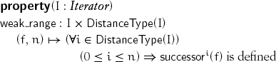
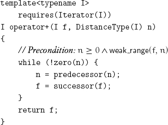
When f is an object of an iterator type and n is an object of the corresponding distance type, we want to be able to define algorithms operating on a weak range ![]() of n iterators beginning with f, using code of the form
of n iterators beginning with f, using code of the form
while (!zero(n)) { n = predecessor(n); ... f = successor(f); }
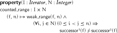
This property enables such an iteration:
Lemma 6.1 0 ≤ j ≤ i ![]() weak_range(f, i)
weak_range(f, i) ![]() weak_range(f, j)
weak_range(f, j)
In a weak range, we can advance up to its size:
The addition of the following axiom ensures that there are no cycles in the range:
When f and l are objects of an iterator type, we want to be able to define algorithms working on a bounded range [f, l) of iterators beginning with f and limited by l, using code of the form
while (f != l) { ... f = successor(f); }
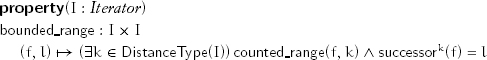
This property enables such an iteration:
The structure of iteration using a bounded range terminates the first time l is encountered; therefore, unlike a weak range, it cannot have cycles.
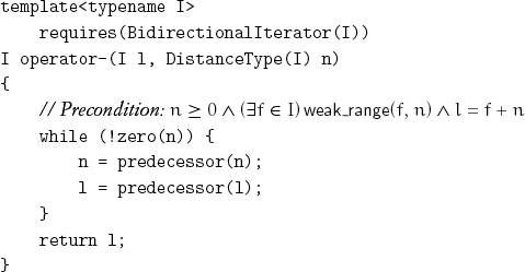
In a bounded range, we can implement[3] a partial subtraction on iterators:
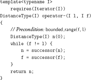
Because successor may not be regular, subtraction should be used only in preconditions or in situations in which we only want to compute the size of a bounded range.
Our definitions of + and – between iterators and integers are not inconsistent with mathematical usage, where + and – are always defined on the same type. As in mathematics, both + between iterators and integers and – between iterators are defined inductively in terms of successor. The standard inductive definition of addition on natural numbers uses the successor function:[4]
a + 0 = a
a + successor(b) = successor(a + b)
Our iterative definition of f + n for iterators is equivalent even though f and n are of different types. As with natural numbers, a variant of associativity is provable by induction.
Lemma 6.2 (f + n)+ m = f +(n + m)
In preconditions we need to specify membership within a range. We borrow conventions from intervals (see Appendix A) to introduce half-open and closed ranges. We use variations of the notation for weak or counted ranges and for bounded ranges.
A half-open weak or counted range ![]() where n ≥ 0 is an integer, denotes the sequence of iterators {successork(f) | 0 ≤ k< n}. A closed weak or counted range
where n ≥ 0 is an integer, denotes the sequence of iterators {successork(f) | 0 ≤ k< n}. A closed weak or counted range ![]() , where n ≥ 0 is an integer, denotes the sequence of iterators {successork (f) | 0 ≤ k ≤ n}.
, where n ≥ 0 is an integer, denotes the sequence of iterators {successork (f) | 0 ≤ k ≤ n}.
A half-open bounded range [f, l) is equivalent to the half-open counted range ![]() . A closed bounded range [f, l] is equivalent to the closed counted range
. A closed bounded range [f, l] is equivalent to the closed counted range ![]() .
.
The size of a range is the number of iterators in the sequence it denotes.
Lemma 6.3 successor is defined for every iterator in a half-open range and for every iterator except the last in a closed range.
If r is a range and i is an iterator, we say that i ![]() r if i is a member of the corresponding set of iterators.
r if i is a member of the corresponding set of iterators.
Lemma 6.4 If i ![]() [f, l), both [f, i) and [i, l) are bounded ranges.
[f, l), both [f, i) and [i, l) are bounded ranges.
Empty half-open ranges are specified by ![]() or [i, i) for some iterator i. There are no empty closed ranges.
or [i, i) for some iterator i. There are no empty closed ranges.
Lemma 6.6 Empty ranges have neither first nor last elements.
It is useful to describe an empty sequence of iterators starting at a particular iterator. For example, binary search looks for the sequence of iterators whose values are equal to a given value. This sequence is empty if there are no such values but is positioned where they would appear if inserted.
An iterator l is called the limit of a half-open bounded range [f, l). An iterator f + n is the limit of a half-open weak range ![]() . Observe that an empty range has a limit even though it does not have a first or last element.
. Observe that an empty range has a limit even though it does not have a first or last element.
Lemma 6.7 The size of a half-open weak range ![]() is n. The size of a closed weak range
is n. The size of a closed weak range ![]() is n + 1. The size of a half-open bounded range [f, l) is l – f. The size of a closed bounded range [f, l] is (l – f)+1.
is n + 1. The size of a half-open bounded range [f, l) is l – f. The size of a closed bounded range [f, l] is (l – f)+1.
If i and j are iterators in a counted or bounded range, we define the relation i ![]() j to mean that i ≠ j
j to mean that i ≠ j ![]() bounded_range (i, j): in other words, that one or more applications of successor leads from i to j. The relation
bounded_range (i, j): in other words, that one or more applications of successor leads from i to j. The relation ![]() (“precedes”) and the corresponding reflexive relation
(“precedes”) and the corresponding reflexive relation ![]() (“precedes or equal”) are used in specifications, such as preconditions and postconditions of algorithms. For many pairs of values of an iterator type,
(“precedes or equal”) are used in specifications, such as preconditions and postconditions of algorithms. For many pairs of values of an iterator type, ![]() is not defined, so there is often no effective way to write code implementing
is not defined, so there is often no effective way to write code implementing ![]() . For example, there is no efficient way to determine whether one node precedes another in a linked structure; the nodes might not even be linked together.
. For example, there is no efficient way to determine whether one node precedes another in a linked structure; the nodes might not even be linked together.
6.4 Readable Ranges
A range of iterators from a type modeling Readable and Iterator is readable if source is defined on all the iterators in the range:
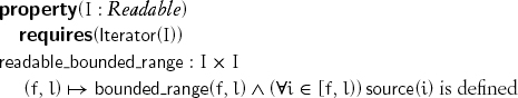
Observe that source need not be defined on the limit of the range. Also, since an iterator may no longer be well-formed after successor is applied, it is not guaranteed that source can be applied to an iterator after its successor has been obtained. readable_weak_range and readable_counted_range are defined similarly.
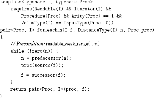
Given a readable range, we could apply a procedure to each value in the range:
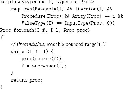
We return the procedure because it could have accumulated useful information during the traversal.[5]
We implement linear search with the following procedure:
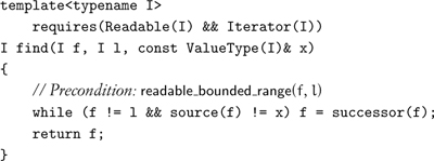
Either the returned iterator is equal to the limit of the range, or its value is equal to x. Returning the limit indicates failure of the search. Since there are n +1 outcomes for a search of a range of size n, the limit serves a useful purpose here and in many other algorithms. A search involving find can be restarted by advancing past the returned iterator and then calling find again.
Changing the comparison with x to use equality instead of inequality gives us find_not.
We can generalize from searching for an equal value to searching for the first value satisfying a unary predicate:
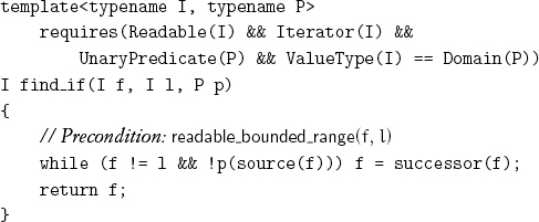
Applying the predicate instead of its complement gives us find_if_not.
Exercise 6.1 Use find_if and find_if_not to implement quantifier functions all, none, not_all, and some, each taking a bounded range and a predicate.
The find and quantifier functions let us search for values satisfying a condition; we can also count the number of satisfying values:
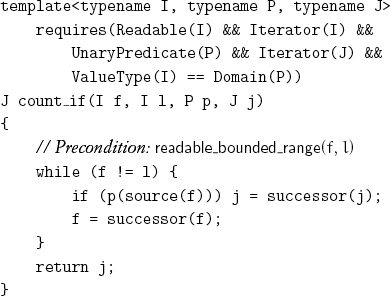
Passing j explicitly is useful when adding an integer to j takes linear time. The type J could be any integer or iterator type, including I.
Exercise 6.2 Implement count_if by passing an appropriate function object to for_each and extracting the accumulation result from the returned function object.
The natural default is to start the count from zero and use the distance type of the iterators:
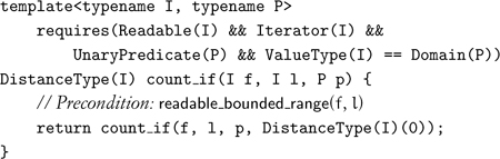
Replacing the predicate with an equality test gives us count; negating the tests gives us count_not and count_if_not.
The notation ![]() for the sum of the ai is frequently generalized to other binary operations; for example,
for the sum of the ai is frequently generalized to other binary operations; for example, ![]() is used for products and
is used for products and ![]() for conjunctions. In each case, the operation is associative, which means that the grouping is not important. Kenneth Iverson unified this notation in the programming language APL with the reduction operator /, which takes a binary operation and a sequence and reduces the elements into a single result.[6] For example, +/1 2 3 equals 6.
for conjunctions. In each case, the operation is associative, which means that the grouping is not important. Kenneth Iverson unified this notation in the programming language APL with the reduction operator /, which takes a binary operation and a sequence and reduces the elements into a single result.[6] For example, +/1 2 3 equals 6.
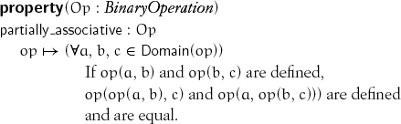
Iverson does not restrict reduction to associative operations. We extend Iverson’s reduction to work on iterator ranges but restrict it to partially associative operations: If an operation is defined between adjacent elements, it can be reassociated:
As an example of an operation that is partially associative but not associative, consider concatenation of two ranges [f0, l0) and [f1, l1), which is defined only when l0 = f1.
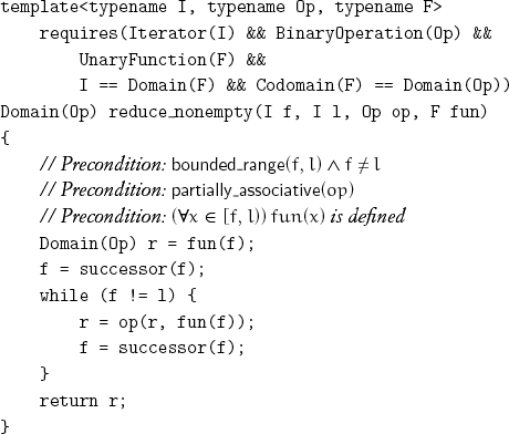
We allow a unary function to be applied to each iterator before the binary operation is performed, obtaining ai from i. Since an arbitrary partially associative operation might not have an identity, we provide a version of reduction requiring a nonempty range:
The natural default for fun is source. An identity element can be passed in to be returned on an empty range:
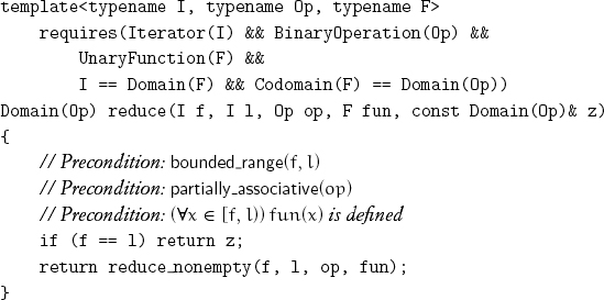
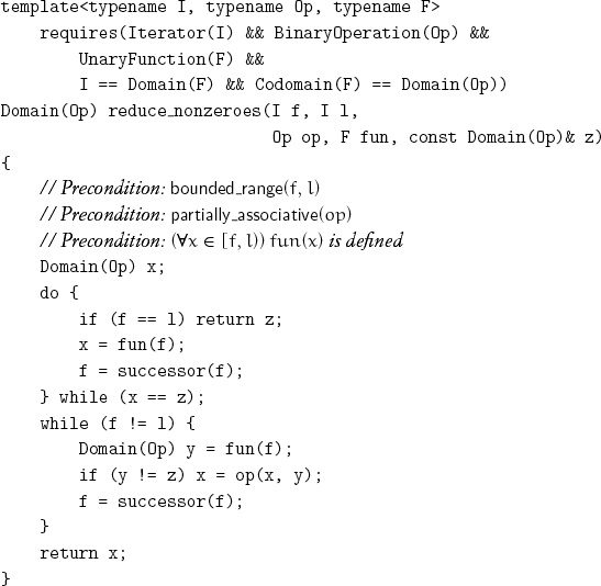
When operations involving the identity element are slow or require extra logic to implement, the following procedure is useful:
Algorithms taking a bounded range have a corresponding version taking a weak or counted range; more information, however, needs to be returned:
The final value of the iterator must be returned because the lack of regularity of successor means that it could not be recomputed. Even for iterators where successor is regular, recomputing it could take time linear in the size of the range.
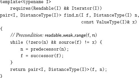
find_n returns the final value of the iterator and the count because both are needed to restart a search.
Exercise 6.3 Implement variations taking a weak range instead of a bounded range of all the versions of find, quantifiers, count, and reduce.
We can eliminate one of the two tests in the loop of find_if when we are assured that an element in the range satisfies the predicate; such an element is called a sentinel:
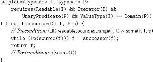
Applying the predicate instead of its complement gives find_if_not_unguarded.
Given two ranges with the same value type and a relation on that value type, we can search for a mismatched pair of values:
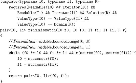
Exercise 6.4 State the postcondition for find_mismatch, and explain why the final values of both iterators are returned.
The natural default for the relation in find_mismatch is the equality on the value type.
Exercise 6.5 Design variations of find_mismatch for all four combinations of counted and bounded ranges.
Sometimes, it is important to find a mismatch not between ranges but between adjacent elements of the same range:
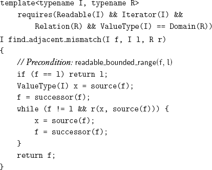
We must copy the previous value because we cannot apply source to an iterator after successor has been applied to it. The weak requirements of Iterator also imply that returning the first iterator in the mismatched pair may return a value that is not well formed.
6.5 Increasing Ranges
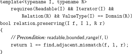
Given a relation on the value type of some iterator, a range over that iterator type is called relation preserving if the relation holds for every adjacent pair of values in the range. In other words, find_adjacent_mismatch will return the limit when called with this range and relation:
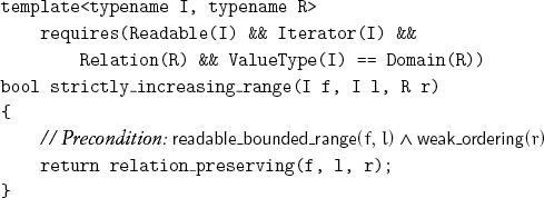
Given a weak ordering r, we say that a range is r-increasing if it is relation preserving with respect to the complement of the converse of r. Given a weak ordering r, we say that a range is strictly r-increasing if it is relation preserving with respect to r.[7] It is straightforward to implement a test for a strictly increasing range:
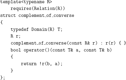
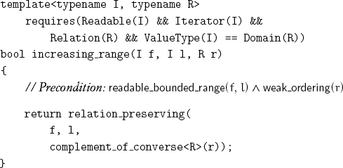
With the help of a function object, we can implement a test for an increasing range:
Defining strictly_increasing_counted_range and increasing_counted_range is straightforward.
Given a predicate p on the value type of some iterator, a range over that iterator type is called p-partitioned if any values of the range satisfying the predicate follow every value of the range not satisfying the predicate. A test that shows whether a range is p-partitioned is straightforward:
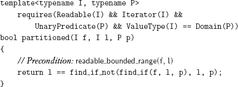
The iterator returned by the call of find_if is called the partition point; it is the first iterator, if any, whose value satisfies the predicate.
Exercise 6.6 Implement the predicate partitioned_n, which tests whether a counted range is p-partitioned.
Linear search must invoke source after each application of successor because a failed test provides no information about the value of any other iterator in the range. However, the uniformity of a partitioned range gives us more information.
Lemma 6.8 If p is a predicate and [f, l) is a p-partitioned range:
![]()
This suggests a bisection algorithm for finding the partition point: Assuming a uniform distribution, testing the midpoint of the range reduces the search space by a factor of 2. However, such an algorithm may need to traverse an already traversed subrange, which requires the regularity of successor.
6.6 Forward Iterators
Making successor regular allows us to pass through the same range more than once and to maintain more than one iterator into the range:
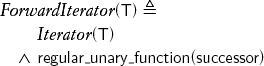
Note that Iterator and ForwardIterator differ only by an axiom; there are no new operations. In addition to successor, all the other functional procedures defined on refinements of the forward iterator concept introduced later in the chapter are regular. The regularity of successor allows us to implement find_adjacent_mismatch without saving the value before advancing:
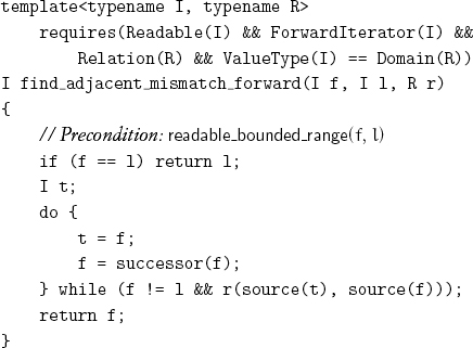
Note that t points to the first element of this mismatched pair and could also be returned.
In Chapter 10 we show how to use concept dispatch to overload versions of an algorithm written for different iterator concepts. Suffixes such as _forward allow us to disambiguate the different versions.
The regularity of successor also allows us to implement the bisection algorithm for finding the partition point:
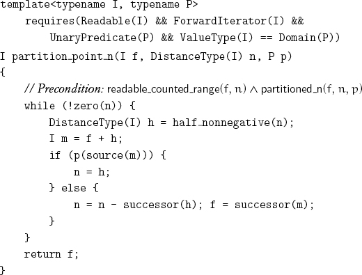
Lemma 6.9 partition_point_n returns the partition point of the p-partitioned range ![]() .
.
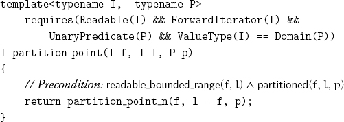
Finding the partition point in a bounded range by bisection[8] requires first finding the size of the range:
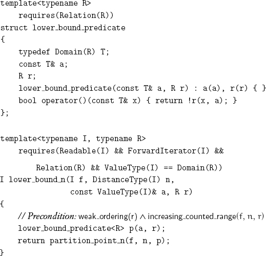
The definition of partition point immediately leads to binary search algorithms on an r-increasing range for a weak ordering r. Any value a, whether or not it appears in the increasing range, determines two iterators in the range called lower bound and upper bound. Informally, a lower bound is the first position where a value equivalent to a could occur in the increasing sequence. Similarly, an upper bound is the successor of the last position where a value equivalent to a could occur. Therefore elements equivalent to a appear only in the half-open range from lower bound to upper bound. For example, assuming total ordering, a sequence with lower bound l and upper bound u for the value a looks like this:
![]()
Note that any of the three regions may be empty.
Lemma 6.10 In an increasing range [f, l), for any value a of the value type of the range, the range is partitioned by the following two predicates:
![]()
That allows us to formally define lower bound and upper bound as the partition points of the corresponding predicates.
Lemma 6.11 The lower-bound iterator precedes or equals the upper-bound iterator.
Implementing a function object corresponding to the predicate leads immediately to an algorithm for determining the lower bound:
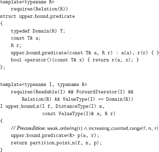
Similarly, for the upper bound:
Exercise 6.7 Implement a procedure that returns both lower and upper bounds and does fewer comparisons than the sum of the comparisons that would be done by calling both lower_bound_n and upper_bound_n.[9]
Applying the predicate in the middle of the range ensures the optimal worst-case number of predicate applications in the partition-point algorithm. Any other choice would be defeated by an adversary who ensures that the larger subrange contains the partition point. Prior knowledge of the expected position of the partition point would lead to probing at that point.
partition_point_n applies the predicate ![]() log2n
log2n![]() + 1 times, since the length of the range is reduced by a factor of 2 at each step. The algorithm performs a logarithmic number of iterator/integer additions.
+ 1 times, since the length of the range is reduced by a factor of 2 at each step. The algorithm performs a logarithmic number of iterator/integer additions.
Lemma 6.12 For a forward iterator, the total number of successor operations performed by the algorithm is less than or equal to the size of the range.
partition_point also calculates l – f, which, for forward iterators, adds another n calls of successor. It is worthwhile to use it on forward iterators, such as linked lists, whenever the predicate application is more expensive than calling successor.
Lemma 6.13 Assuming that the expected distance to the partition point is equal to half the size of the range, partition_point is faster than find_if on finding the partition point for forward iterators whenever
![]()
6.7 Indexed Iterators
In order for partition_point, lower_bound, and upper_bound to dominate linear search, we need to ensure that adding an integer to an iterator and subtracting an iterator from an iterator are fast:
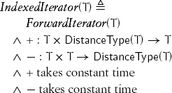
The operations + and –, which were defined for Iterator in terms of successor, are now required to be primitive and fast: This concept differs from ForwardIterator only by strengthening complexity requirements. We expect the cost of + and – on indexed iterators to be essentially identical to the cost of successor.
6.8 Bidirectional Iterators
There are situations in which indexing is not possible, but we have the ability to go backward:
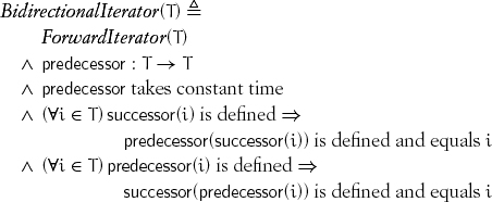
As with successor, predecessor does not have to be total; the axioms of the concept relate its definition space to that of successor. We expect the cost of predecessor to be essentially identical to the cost of successor.
Lemma 6.14 If successor is defined on bidirectional iterators i and j,
successor(i) = successor(j) ![]() i = j
i = j
In a weak range of bidirectional iterators, movement backward as far as the beginning of the range is possible:
With bidirectional iterators, we can search backward. As we noted earlier, when searching a range of n iterators, there are n + 1 outcomes; this is true whether we search forward or backward. So we need a convention for representing half-open on left ranges of the form (f, l]. To indicate “not found,” we return f, which forces us to return successor (i) if we find a satisfying element at iterator i:
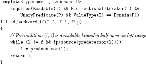
Comparing this with find_if illustrates a program transformation: f and l interchange roles, source (i) becomes source (predecessor (i)), and successor (i) becomes predecessor (i). Under this transformation, in a nonempty range, l is dereferenceable, but f is not.
The program transformation just demonstrated can be applied to any algorithm that takes a range of forward iterators. Thus it is possible to implement an adapter type that, given a bidirectional iterator type, produces another bidirectional iterator type where successor becomes predecessor, predecessor becomes successor, and source becomes source of predecessor.[10] This adapter type allows any algorithm on iterators or forward iterators to work backward on bidirectional iterators, and it also allows any algorithm on bidirectional iterators to interchange the traversal directions.
Exercise 6.8 Rewrite find_backward_if with only one call of predecessor in the loop.
Exercise 6.9 As an example of an algorithm that uses both successor and predecessor, implement a predicate that determines whether a range is a palindrome: It reads the same way forward and backward.
6.9 Random-Access Iterators
Some iterator types satisfy the requirements of both indexed and bidirectional iterators. These types, called random-access iterators, provide the full power of computer addresses:
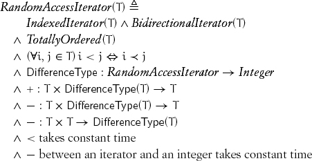
DifferenceType (T) is large enough to contain distances and their additive inverses; if i and j are iterators from a valid range, i – j is always defined. It is possible to add a negative integer to, or subtract it from, an iterator.
On weaker iterator types, the operations + and – are only defined within one range. For random-access iterator types, this holds for < as well as for + and –. In general, an operation on two iterators is defined only when they belong to the same range.
Project 6.1 Define axioms relating the operations of random-access iterators to each other.
We do not describe random-access iterators in great detail, because of the following.
Theorem 6.1 For any procedure defined on an explicitly given range of random-access iterators, there is another procedure defined on indexed iterators with the same complexity.
Proof: Since the operations on random-access iterators are only defined on iterators belonging to the same range, it is possible to implement an adapter type that, given an indexed iterator type, produces a random-access iterator type. The state of such an iterator contains an iterator f and an integer i and represents the iterator f + i. The iterator operations, such as +, –, and <, operate on i; source operates on f + i. In other words, an iterator pointing to the beginning of the range, together with an index into the range, behave like a random-access iterator.
The theorem shows the theoretical equivalence of these concepts in any context in which the beginnings of ranges are known. In practice, we have found that there is no performance penalty for using the weaker concept. In some cases, however, a signature needs to be adjusted to include the beginning of the range.
Project 6.2 Implement a family of abstract procedures for finding a subsequence within a sequence. Describe the tradeoffs for selecting an appropriate algorithm.[11]
6.10 Conclusions
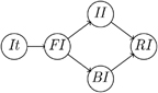
Algebra provides us with a hierarchy of concepts, such as semigroups, monoids, and groups, that allows us to state algorithms in the most general context. Similarly, the iterator concepts (Figure 6.1) allow us to state algorithms on sequential data structures in their most general context. The development of these concepts used three kinds of refinement: adding an operation, strengthening semantics, and tightening complexity requirement. In particular, the three concepts iterator, forward iterator, and indexed iterator differ not by their operations but only by their semantics and complexity. A variety of search algorithms for different iterator concepts, counted and bounded ranges, and range ordering serve as the foundation of sequential programming.
Figure 6.1. Iterator concepts.