
Chapter 2
Transformations and Their Orbits
This chapter defines a transformation as a unary regular function from a type to itself. Successive applications of a transformation starting from an initial value determine an orbit of this value. Depending only on the regularity of the transformation and the finiteness of the orbit, we implement an algorithm for determining orbit structures that can be used in different domains. For example, it could be used to detect a cycle in a linked list or to analyze a pseudorandom number generator. We derive an interface to the algorithm as a set of related procedures and definitions for their arguments and results. This analysis of an orbit-structure algorithm allows us to introduce our approach to programming in the simplest possible setting.
2.1 Transformations
While there are functions from any sequence of types to any type, particular classes of signatures commonly occur. In this book we frequently use two such classes: homogeneous predicates and operations. Homogeneous predicates are of the form T × ... × T → bool; operations are functions of the form T × ... × T → T. While there are n-ary predicates and n-ary operations, we encounter mostly unary and binary homogeneous predicates and unary and binary operations.
A predicate is a functional procedure returning a truth value:
A homogeneous predicate is one that is also a homogeneous function:
A unary predicate is a predicate taking one parameter:
An operation is a homogeneous function whose codomain is equal to its domain:
Examples of operations:
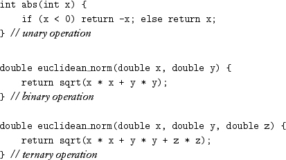
Lemma 2.1 euclidean_norm(x, y, z) = euclidean_norm(euclidean_norm(x, y), z)
This lemma shows that the ternary version can be obtained from the binary version. For reasons of efficiency, expressiveness, and, possibly, accuracy, the ternary version is part of the computational basis for programs dealing with three-dimensional space.
A procedure is partial if its definition space is a subset of the direct product of the types of its inputs; it is total if its definition space is equal to the direct product. We follow standard mathematical usage, where partial function includes total function. We call partial procedures that are not total nontotal. Implementations of some total functions are nontotal on the computer because of the finiteness of the representation. For example, addition on signed 32-bit integers is nontotal.
A nontotal procedure is accompanied by a precondition specifying its definition space. To verify the correctness of a call of that procedure, we must determine that the arguments satisfy the precondition. Sometimes, a partial procedure is passed as a parameter to an algorithm that needs to determine at runtime the definition space of the procedural parameter. To deal with such cases, we define a definition-space predicate with the same inputs as the procedure; the predicate returns true if and only if the inputs are within the definition space of the procedure. Before a nontotal procedure is called, either its precondition must be satisfied, or the call must be guarded by a call of its definition-space predicate.
Exercise 2.1 Implement a definition-space predicate for addition on 32-bit signed integers.
This chapter deals with unary operations, which we call transformations:
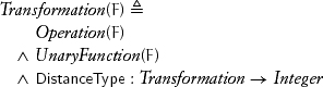
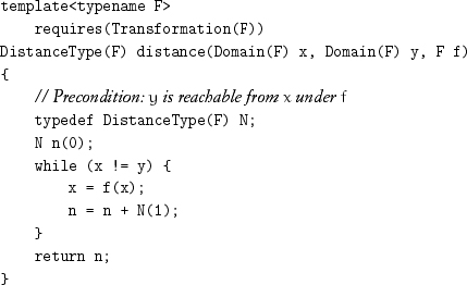
We discuss DistanceType in the next section.
Transformations are self-composable: f(x), f(f(x)), f(f(f(x))), and so on. The definition space of f(f(x)) is the intersection of the definition space and result space of f. This ability to self-compose, together with the ability to test for equality, allows us to define interesting algorithms.
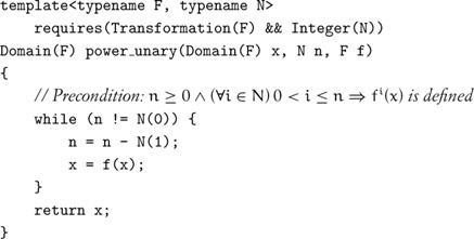
When f is a transformation, we define its powers as follows:
![]()
To implement an algorithm to compute fn(x), we need to specify the requirement for an integer type. We study various concepts describing integers in Chapter 5. For now we rely on the intuitive understanding of integers. Their models include signed and unsigned integral types, as well as arbitrary-precision integers, with these operations and literals:
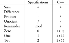
where I is an integer type.
That leads to the following algorithm:
2.2 Orbits
To understand the global behavior of a transformation, we examine the structure of its orbits: elements reachable from a starting element by repeated applications of the transformation. y is reachable from x under a transformation f if for some n ≥ 0, y = fn(x). x is cyclic under f if for some n ≥ 1, x = fn(x). x is terminal under f if and only if x is not in the definition space of f. The orbit of x under a transformation f is the set of all elements reachable from x under f.
Lemma 2.2 An orbit does not contain both a cyclic and a terminal element.
Lemma 2.3 An orbit contains at most one terminal element.
If y is reachable from x under f, the distance from x to y is the least number of transformation steps from x to y. Obviously, distance is not always defined.
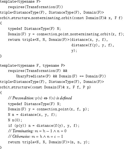
Given a transformation type F, DistanceType(F) is an integer type large enough to encode the maximum number of steps by any transformation f ![]() F from one element of T = Domain(F) to another. If type T occupies k bits, there can be as many as 2k values but only 2k – 1 steps between distinct values. Thus if T is a fixed-size type, an integral type of the same size is a valid distance type for any transformation on T. (Instead of using the distance type, we allow the use of any integer type in power_unary, since the extra generality does not appear to hurt there.) It is often the case that all transformation types over a domain have the same distance type. In this case the type function DistanceType is defined for the domain type and defines the corresponding type function for the transformation types.
F from one element of T = Domain(F) to another. If type T occupies k bits, there can be as many as 2k values but only 2k – 1 steps between distinct values. Thus if T is a fixed-size type, an integral type of the same size is a valid distance type for any transformation on T. (Instead of using the distance type, we allow the use of any integer type in power_unary, since the extra generality does not appear to hurt there.) It is often the case that all transformation types over a domain have the same distance type. In this case the type function DistanceType is defined for the domain type and defines the corresponding type function for the transformation types.
The existence of DistanceType leads to the following procedure:
Orbits have different shapes. An orbit of x under a transformation is
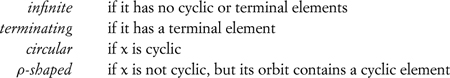
An orbit of x is finite if it is not infinite. Figure 2.1 illustrates the various cases.
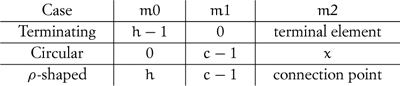
The orbit cycle is the set of cyclic elements in the orbit and is empty for infinite and terminating orbits. The orbit handle, the complement of the orbit cycle with respect to the orbit, is empty for a circular orbit. The connection point is the first cyclic element, and is the first element of a circular orbit and the first element after the handle for a ρ-shaped orbit. The orbit size o of an orbit is the number of distinct elements in it. The handle size h of an orbit is the number of elements in the orbit handle. The cycle size c of an orbit is the number of elements in the orbit cycle.
Lemma 2.5 The distance from any point in an orbit to a point in a cycle of that orbit is always defined.
Lemma 2.6 If x and y are distinct points in a cycle of size c,
c = distance(x, y, f) + distance (y, x, f)
Lemma 2.7 If x and y are points in a cycle of size c, the distance from x to y satisfies
0 ≤ distance (x, y, f) < c
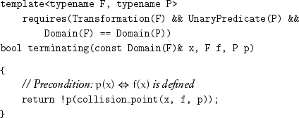
2.3 Collision Point
If we observe the behavior of a transformation, without access to its definition, we cannot determine whether a particular orbit is infinite: It might terminate or cycle back at any point. If we know that an orbit is finite, we can use an algorithm to determine the shape of the orbit. Therefore there is an implicit precondition of orbit finiteness for all the algorithms in this chapter.
There is, of course, a naive algorithm that stores every element visited and checks at every step whether the new element has been previously encountered. Even if we could use hashing to speed up the search, such an algorithm still would require linear storage and would not be practical in many applications. However, there is an algorithm that requires only a constant amount of storage.
The following analogy helps to understand the algorithm. If a fast car and a slow one start along a path, the fast one will catch up with the slow one if and only if there is a cycle. If there is no cycle, the fast one will reach the end of the path before the slow one. If there is a cycle, by the time the slow one enters the cycle, the fast one will already be there and will catch up eventually. Carrying our intuition from the continuous domain to the discrete domain requires care to avoid the fast one skipping past the slow one.[1]
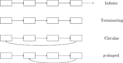
The discrete version of the algorithm is based on looking for a point where fast meets slow. The collision point of a transformation f and a starting point x is the unique y such that
y = fn(x) = f2n+1(x)
and n ≥ 0 is the smallest integer satisfying this condition. This definition leads to an algorithm for determining the orbit structure that needs one comparison of fast and slow per iteration. To handle partial transformations, we pass a definition-space predicate to the algorithm:
We establish the correctness of collision_point in three stages: (1) verifying that it never applies f to an argument outside the definition space; (2) verifying that if it terminates, the postcondition is satisfied; and (3) verifying that it always terminates.
While f is a partial function, its use by the procedure is well defined, since the movement of fast is guarded by a call of p. The movement of slow is unguarded, because by the regularity of f, slow traverses the same orbit as fast, so f is always defined when applied to slow.
The annotations show that if, after n ≥ 0 iterations, fast becomes equal to slow, then fast = f2n+1(x) and slow = fn(x). Moreover, n is the smallest such integer, since we checked the condition for every i < n.
If there is no cycle, p will eventually return false because of finiteness. If there is a cycle, slow will eventually reach the connection point (the first element in the cycle). Consider the distance d from fast to slow at the top of the loop when slow first enters the cycle: 0 ≤ d < c. If d = 0, the procedure terminates. Otherwise the distance from fast to slow decreases by 1 on each iteration. Therefore the procedure always terminates; when it terminates, slow has moved a total of h + d steps.
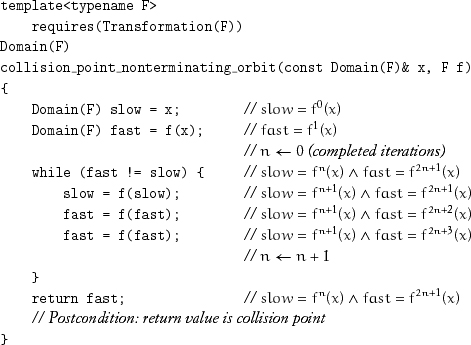
The following procedure determines whether an orbit is terminating:
Sometimes we know either that the transformation is total or that the orbit is nonterminating for a particular starting element. For these situations it is useful to have a specialized version of collision_point:
In order to determine the cycle structure—handle size, connection point, and cycle size—we need to analyze the position of the collision point.
When the procedure returns the collision point
fn(x) = f2n+1(x)
n is the number of steps taken by slow, and 2n + 1 is the number of steps taken by fast.
n = h + d
where h is the handle size and 0 ≤ d < c is the number of steps taken by slow inside the cycle. The number of steps taken by fast is
2n +1 = h + d + qc
where q > 0 is the number of full cycles completed by fast when it collides with slow. Since n = h + d,
2(h + d)+1 = h + d + qc
Simplifying gives
qc = h + d + 1
Let us represent h modulo c:
h = mc + r
with 0 ≤ r < c. Substitution gives
qc = mc + r + d + 1
or
d = (q – m)c – r – 1
0 ≤ d < c implies
q – m = 1
so
d = c – r – 1
and r + 1 steps are needed to complete the cycle.
Therefore the distance from the collision point to the connection point is
e = r +1
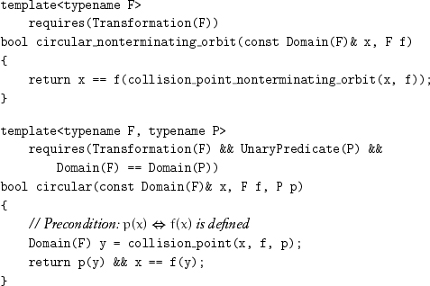
In the case of a circular orbit h = 0, r = 0, and the distance from the collision point to the beginning of the orbit is
e = 1
Circularity, therefore, can be checked with the following procedures:
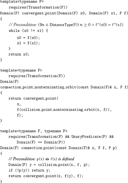
We still don’t know the handle size h and the cycle size c. Determining the latter is simple once the collision point is known: Traverse the cycle and count the steps.
To see how to determine h, let us look at the position of the collision point:
fh+d(x) = fh+c-r-1(x) = fmc+r+c-r-1(x) = f(m+1)c-1(x)
Taking h + 1 steps from the collision point gets us to the point f(m+1)c+h(x), which equals fh(x), since (m + 1)c corresponds to going around the cycle m + 1 times. If we simultaneously take h steps from x and h + 1 steps from the collision point, we meet at the connection point. In other words, the orbits of x and 1 step past the collision point converge in exactly h steps, which leads to the following sequence of algorithms:
Lemma 2.8 If the orbits of two elements intersect, they have the same cyclic elements.
Exercise 2.2 Design an algorithm that determines, given a transformation and its definition-space predicate, whether the orbits of two elements intersect.
Exercise 2.3 The precondition of convergent_point ensures termination. Implement an algorithm convergent_point_guarded for use when that precondition is not known to hold, but there is an element in common to the orbits of both x0 and x1.
2.4 Measuring Orbit Sizes
The natural type to use for the sizes o, h, and c of an orbit on type T would be an integer count type large enough to count all the distinct values of type T. If a type T occupies k bits, there can be as many as 2k values, so a count type occupying k bits could not represent all the counts from 0 to 2k. There is a way to represent these sizes by using distance type.
An orbit could potentially contain all values of a type, in which case o might not fit in the distance type. Depending on the shape of such an orbit, h and c would not fit either. However, for a ρ-shaped orbit, both h and c fit. In all cases each of these fits: o – 1 (the maximum distance in the orbit), h – 1 (the maximum distance in the handle), and c – 1 (the maximum distance in the cycle). That allows us to implement procedures returning a triple representing the complete structure of an orbit, where the members of the triple are as follows:
Exercise 2.4 Derive formulas for the count of different operations (f, p, equality) for the algorithms in this chapter.
Exercise 2.5 Use orbit_structure_nonterminating_orbit to determine the average handle size and cycle size of the pseudorandom number generators on your platform for various seeds.
2.5 Actions
Algorithms often use a transformation f in a statement like
x = f(x);
Changing the state of an object by applying a transformation to it defines an action on the object. There is a duality between transformations and the corresponding actions: An action is definable in terms of a transformation, and vice versa:
void a(T& x) { x = f(x); } // action from transformation
and
T f(T x) { a(x); return x; } // transformation from action
Despite this duality, independent implementations are sometimes more efficient, in which case both action and transformation need to be provided. For example, if a transformation is defined on a large object and modifies only part of its overall state, the action could be considerably faster.
Exercise 2.6 Rewrite all the algorithms in this chapter in terms of actions.
Project 2.1 Another way to detect a cycle is to repeatedly test a single advancing element for equality with a stored element while replacing the stored element at ever-increasing intervals. This and other ideas are described in Sedgewick, et al. [1979], Brent [1980], and Levy [1982]. Implement other algorithms for orbit analysis, compare their performance for different applications, and develop a set of recommendations for selecting the appropriate algorithm.
2.6 Conclusions
Abstraction allowed us to define abstract procedures that can be used in different domains. Regularity of types and functions is essential to make the algorithms work: fast and slow follow the same orbit because of regularity. Developing nomenclature is essential (e.g., orbit kinds and sizes). Affiliated types, such as distance type, need to be precisely defined.