Chapter 2. The Big Picture
Often the best path to understanding a given task is to have a good grasp of the big picture. Many fundamental concepts can present challenges to the newcomer to embedded systems development. This chapter takes you on a tour of a typical embedded system and the development environment with specific emphasis on the concepts and components that make developing these systems unique and often challenging.
2.1 Embedded or Not?
Several key attributes are associated with embedded systems. You wouldn’t necessarily call your desktop PC an embedded system. But consider a desktop PC hardware platform in a remote data center that performs a critical monitoring and alarm task. Assume that this data center normally is not staffed. This imposes a different set of requirements on this hardware platform. For example, if power is lost and then restored, you would expect this platform to resume its duties without operator intervention.
Embedded systems come in a variety of shapes and sizes, from the largest multiple-rack data storage or networking powerhouses to tiny modules such as your personal MP3 player or cellular handset. Following are some of the usual characteristics of an embedded system:
• Contains a processing engine, such as a general-purpose microprocessor.
• Typically designed for a specific application or purpose.
• Includes a simple (or no) user interface, such as an automotive engine ignition controller.
• Often is resource-limited. For example, it might have a small memory footprint and no hard drive.
• Might have power limitations, such as a requirement to operate from batteries.
• Not typically used as a general-purpose computing platform.
• Generally has application software built in, not user-selected.
• Ships with all intended application hardware and software preintegrated.
• Often is intended for applications without human intervention.
Most commonly, embedded systems are resource-constrained compared to the typical desktop PC. Embedded systems often have limited memory, small or no hard drives, and sometimes no external network connectivity. Frequently, the only user interface is a serial port and some LEDs. These and other issues can present challenges to the embedded system developer.
2.1.1 BIOS Versus Bootloader
When power is first applied to the desktop computer, a software program called the BIOS immediately takes control of the processor. (Historically, BIOS was an acronym meaning Basic Input/Output Software, but the term has taken on a meaning of its own as the functions it performs have become much more complex than the original implementations.) The BIOS might actually be stored in Flash memory (described shortly) to facilitate field upgrade of the BIOS program itself.
The BIOS is a complex set of system-configuration software routines that have knowledge of the low-level details of the hardware architecture. Most of us are unaware of the extent of the BIOS and its functionality, but it is a critical piece of the desktop computer. The BIOS first gains control of the processor when power is applied. Its primary responsibility is to initialize the hardware, especially the memory subsystem, and load an operating system from the PC’s hard drive.
In a typical embedded system (assuming that it is not based on an industry-standard x86 PC hardware platform), a bootloader is the software program that performs the equivalent functions. In your own custom embedded system, part of your development plan must include the development of a bootloader specific to your board. Luckily, several good open source bootloaders are available that you can customize for your project. These are introduced in Chapter 7, “Bootloaders.”
Here are some of the more important tasks your bootloader performs on power-up:
• Initializes critical hardware components, such as the SDRAM controller, I/O controllers, and graphics controllers.
• Initializes system memory in preparation for passing control to the operating system.
• Allocates system resources such as memory and interrupt circuits to peripheral controllers, as necessary.
• Provides a mechanism for locating and loading your operating system image.
• Loads and passes control to the operating system, passing any required startup information. This can include total memory size, clock rates, serial port speeds, and other low-level hardware-specific configuration data.
This is a simplified summary of the tasks that a typical embedded-system bootloader performs. The important point to remember is this: If your embedded system will be based on a custom-designed platform, these bootloader functions must be supplied by you, the system designer. If your embedded system is based on a commercial off-the-shelf (COTS) platform such as an ATCA chassis,1 the bootloader (and often the Linux kernel) typically is included on the board. Chapter 7 discusses bootloaders in more detail.
2.2 Anatomy of an Embedded System
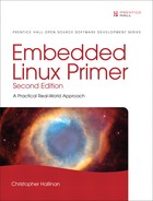
Figure 2-1 is a block diagram of a typical embedded system. This is a simple example of a high-level hardware architecture that might be found in a wireless access point. The system is architected around a 32-bit RISC processor. Flash memory is used for nonvolatile program and data storage. Main memory is synchronous dynamic random-access memory (SDRAM) and might contain anywhere from a few megabytes to hundreds of megabytes, depending on the application. A real-time clock module, often backed up by battery, keeps the time of day (calendar/wall clock, including date). This example includes an Ethernet and USB interface, as well as a serial port for console access via RS-232. The 802.11 chipset or module implements the wireless modem function.
Figure 2-1. Embedded system
Often the processor in an embedded system performs many functions beyond the traditional core instruction stream processing. The hypothetical processor shown in Figure 2-1 contains an integrated UART for a serial interface and integrated USB and Ethernet controllers. Many processors contain integrated peripherals. Sometimes they are referred to as system on chip (SOC). We look at several examples of integrated processors in Chapter 3, “Processor Basics.”
2.2.1 Typical Embedded Linux Setup
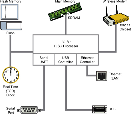
Often the first question posed by the newcomer to embedded Linux is, just what do you need to begin development? To answer that question, Figure 2-2 shows a typical embedded Linux development setup.
Figure 2-2. Embedded Linux development setup
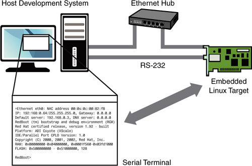
Figure 2-2 is a common arrangement. It shows a host development system, running your favorite desktop Linux distribution, such as Red Hat, SUSE, or Ubuntu Linux. The embedded Linux target board is connected to the development host via an RS-232 serial cable. You plug the target board’s Ethernet interface into a local Ethernet hub or switch, to which your development host is also attached via Ethernet. The development host contains your development tools and utilities along with target files, which normally are obtained from an embedded Linux distribution.
For this example, our primary connection to the embedded Linux target is via the RS-232 connection. A serial terminal program is used to communicate with the target board. Minicom is one of the most commonly used serial terminal applications and is available on virtually all desktop Linux distributions.2 The author has switched to using screen as his terminal of choice, replacing the functionality of minicom. It offers much more flexibility, especially for capturing traces, and it’s more forgiving of serial line garbage often encountered during system bringup or troubleshooting. To use screen in this manner on a USB-attached serial dongle, simply invoke it on your serial terminal and specify the speed:
$ screen /dev/ttyUSB0 115200
2.2.2 Starting the Target Board
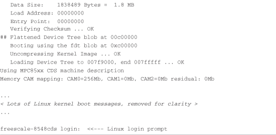
When power is first applied, a bootloader supplied with your target board takes immediate control of the processor. It performs some very low-level hardware initialization, including processor and memory setup, initialization of the UART controlling the serial port, and initialization of the Ethernet controller. Listing 2-1 displays the characters received from the serial port, resulting from power being applied to the target. For this example, we have chosen a target board from Freescale Semiconductor, the PowerQUICC III MPC8548 Configurable Development System (CDS). It contains the MPC8548 PowerQUICC III processor. It ships from Freescale with the U-Boot bootloader preinstalled.
Listing 2-1. Initial Bootloader Serial Output
When power is applied to the MPC8548CDS board, U-Boot performs some low-level hardware initialization, which includes configuring a serial port. It then prints a banner line, as shown in the first line of Listing 2-1. Next the CPU and core are displayed, followed by some configuration data describing clocks and cache configuration. This is followed by a text string describing the board.
When the initial hardware configuration is complete, U-Boot configures any hardware subsystems as directed by its static configuration. Here we see I2C, DRAM, FLASH, L2 cache, PCI, and network subsystems being configured by U-Boot. Finally, U-Boot waits for input from the console over the serial port, as indicated by the => prompt.
2.2.3 Booting the Kernel
Now that U-Boot has initialized the hardware, serial port, and Ethernet network interfaces, it has only one job left in its short but useful life span: to load and boot the Linux kernel. All bootloaders have a command to load and execute an operating system image. Listing 2-2 shows one of the more common ways U-Boot is used to manually load and boot a Linux kernel.
Listing 2-2. Loading the Linux Kernel

The tftp command at the start of Listing 2-2 instructs U-Boot to load the kernel image uImage into memory over the network using the TFTP3 protocol. The kernel image, in this case, is located on the development workstation (usually the same machine that has the serial port connected to the target board). The tftp command is passed an address that is the physical address in the target board’s memory where the kernel image will be loaded. Don’t worry about the details now; Chapter 7 covers U-Boot in much greater detail.
The second invocation of the tftp command loads a board configuration file called a device tree. It is referred to by other names, including flat device tree and device tree binary or dtb. You will learn more about this file in Chapter 7. For now, it is enough for you to know that this file contains board-specific information that the kernel requires in order to boot the board. This includes things such as memory size, clock speeds, onboard devices, buses, and Flash layout.
Next, the bootm (boot from memory image) command is issued, to instruct U-Boot to boot the kernel we just loaded from the address specified by the tftp command. In this example of using the bootm command, we instruct U-Boot to load the kernel that we put at 0x600000 and pass the device tree binary (dtb) we loaded at 0xc00000 to the kernel. This command transfers control to the Linux kernel. Assuming that your kernel is properly configured, this results in booting the Linux kernel to a console command prompt on your target board, as shown by the login prompt.
Note that the bootm command is the death knell for U-Boot. This is an important concept. Unlike the BIOS in a desktop PC, most embedded systems are architected in such a way that when the Linux kernel takes control, the bootloader ceases to exist. The kernel claims any memory and system resources that the bootloader previously used. The only way to pass control back to the bootloader is to reboot the board.
One final observation is worth noting. All the serial output in Listing 2-2 up to and including this line is produced by the U-Boot bootloader:
Loading Device Tree to 007f9000, end 007fffff ... OK
The rest of the boot messages are produced by the Linux kernel. We’ll have much more to say about this later, but it is worth noting where U-Boot leaves off and where the Linux kernel image takes over.
2.2.4 Kernel Initialization: Overview
When the Linux kernel begins execution, it spews out numerous status messages during its rather comprehensive boot process. In the example being discussed here, the Linux kernel displayed approximately 200 printk4 lines before it issues the login prompt. (We omitted them from the listing to clarify the point being discussed.) Listing 2-3 reproduces the last several lines of output before the login prompt. The goal of this exercise is not to delve into the details of the kernel initialization (this is covered in Chapter 5, “Kernel Initialization”). The goal is to gain a high-level understanding of what is happening and what components are required to boot a Linux kernel on an embedded system.
Listing 2-3. Linux Final Boot Messages
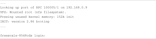
Shortly before issuing a login prompt on the serial terminal, Linux mounts a root file system. In Listing 2-3, Linux goes through the steps required to mount its root file system remotely (via Ethernet) from an NFS5 server on a machine with the IP address 192.168.0.9. Usually, this is your development workstation. The root file system contains the application programs, system libraries, and utilities that make up a Linux system.
The important point in this discussion should not be understated: Linux requires a file system. Many legacy embedded operating systems did not require a file system. This fact is a frequent surprise to engineers making the transition from legacy embedded OSs to embedded Linux. A file system consists of a predefined set of system directories and files in a specific layout on a hard drive or other medium that the Linux kernel mounts as its root file system.
Note that Linux can mount a root file system from other devices. The most common, of course, is to mount a partition from a hard drive as the root file system, as is done on your Linux laptop or workstation. Indeed, NFS is pretty useless when you ship your embedded Linux widget out the door and away from your development environment. However, as you progress through this book, you will come to appreciate the power and flexibility of NFS root mounting as a development environment.
2.2.5 First User Space Process: init
Another important point should be made before we move on. Notice in Listing 2-3 this line:
INIT: version 2.86 booting
Until this point, the kernel itself was executing code, performing the numerous initialization steps in a context known as kernel context. In this operational state, the kernel owns all system memory and operates with full authority over all system resources. The kernel has access to all physical memory and to all I/O subsystems. It executes code in kernel virtual address space, using a stack created and owned by the kernel itself.
When the Linux kernel has completed its internal initialization and mounted its root file system, the default behavior is to spawn an application program called init. When the kernel starts init, it is said to be running in user space or user space context. In this operational mode, the user space process has restricted access to the system and must use kernel system calls to request kernel services such as device and file I/O. These user space processes, or programs, operate in a virtual memory space picked at random6 and managed by the kernel. The kernel, in cooperation with specialized memory-management hardware in the processor, performs virtual-to-physical address translation for the user space process. The single biggest benefit of this architecture is that an error in one process can’t trash the memory space of another. This is a common pitfall in legacy embedded OSs that can lead to bugs that are some of the most difficult to track down.
Don’t be alarmed if these concepts seem foreign. The objective of this section is to paint a broad picture from which you will develop more detailed knowledge as you progress through the book. These and other concepts are covered in great detail in later chapters.
2.3 Storage Considerations
One of the most challenging aspects of embedded Linux development is that most embedded systems have limited physical resources. Although the Core™ 2 Duo machine on your desktop might have 500GB of hard drive space, it is not uncommon to find embedded systems with a fraction of that amount. In many cases, the hard drive typically is replaced by smaller and less expensive nonvolatile storage devices. Hard drives are bulky, have rotating parts, are sensitive to physical shock, and require multiple power supply voltages, which makes them unsuitable for many embedded systems.
2.3.1 Flash Memory
Nearly everyone is familiar with Compact Flash and SD cards used in a wide variety of consumer devices, such as digital cameras and PDAs (both great examples of embedded systems). These modules, based on Flash memory technology, can be thought of as solid-state hard drives, capable of storing many megabytes—and even gigabytes—of data in a tiny footprint. They contain no moving parts, are relatively rugged, and operate on a single common power supply voltage.
Several manufacturers of Flash memory exist. Flash memory comes in a variety of electrical formats, physical packages, and capacities. It is not uncommon to see embedded systems with as little as 4MB or 8MB of nonvolatile storage. More typical storage requirements for embedded Linux systems range from 16MB to 256MB or more. An increasing number of embedded Linux systems have nonvolatile storage into the gigabyte range.
Flash memory can be written to and erased under software control. Rotational hard drive technology remains the fastest writable medium. Flash writing and erasing speeds have improved considerably over time, although Flash write and erase time is still considerably slower. You must understand some fundamental differences between hard drive and Flash memory technology to properly use the technology.
Flash memory is divided into relatively large erasable units, referred to as erase blocks. One of the defining characteristics of Flash memory is how data in Flash is written and erased. In a typical NOR7 Flash memory chip, data can be changed from a binary 1 to a binary 0 under software control using simple data writes directly to the cell’s address, one bit or word at a time. However, to change a bit from a 0 back to a 1, an entire erase block must be erased using a special sequence of control instructions to the Flash chip.
A typical NOR Flash memory device contains many erase blocks. For example, a 4MB Flash chip might contain 64 erase blocks of 64KB each. Flash memory is also available with nonuniform erase block sizes, to facilitate flexible data-storage layouts. These are commonly called boot block or boot sector Flash chips. Often the bootloader is stored in the smaller blocks, and the kernel and other required data are stored in the larger blocks. Figure 2-3 illustrates the block size layout for a typical top boot Flash.
Figure 2-3. Boot block Flash architecture

To modify data stored in a Flash memory array, the block in which the modified data resides must be completely erased. Even if only 1 byte in a block needs to be changed, the entire block must be erased and rewritten.8 Flash block sizes are relatively large compared to traditional hard-drive sector sizes. In comparison, a typical high-performance hard drive has writable sectors of 512 or 1024 bytes. The ramifications of this might be obvious: Write times for updating data in Flash memory can be many times that of a hard drive, due in part to the relatively large quantity of data that must be erased and written back to the Flash for each update. In the worst case, these write cycles can take several seconds.
Another limitation of Flash memory that must be considered is Flash memory cell write lifetime. A NOR Flash memory cell has a limited number of write cycles before failure. Although the number of cycles is fairly large (100,000 cycles per block is typical), it is easy to imagine a poorly designed Flash storage algorithm (or even a bug) that can quickly destroy Flash devices. It goes without saying that you should avoid configuring your system loggers to output to a Flash-based device.
2.3.2 NAND Flash
NAND Flash is a relatively new Flash technology. When NAND Flash hit the market, traditional Flash memory such as that described in the preceding section was called NOR Flash. These distinctions relate to the internal Flash memory cell architecture. NAND Flash devices improve on some of the limitations of traditional (NOR) Flash by offering smaller block sizes, resulting in faster and more efficient writes and generally more efficient use of the Flash array.
NOR Flash devices interface to the microprocessor in a fashion similar to many microprocessor peripherals. That is, they have a parallel data and address bus that are connected directly9 to the microprocessor data/address bus. Each byte or word in the Flash array can be individually addressed in a random fashion. In contrast, NAND devices are accessed serially through a complex interface that varies among vendors. NAND devices present an operational model more similar to that of a traditional hard drive and associated controller. Data is accessed in serial bursts, which are far smaller than NOR Flash block size. Write cycle lifetime for NAND Flash is an order of magnitude greater than for NOR Flash, although erase times are significantly smaller.
In summary, NOR Flash can be directly accessed by the microprocessor, and code can even be executed directly out of NOR Flash. (However, for performance reasons, this is rarely done, and then only on systems in which resources are extremely scarce.) In fact, many processors cannot cache instruction accesses to Flash, as they can with DRAM. This further degrades execution speed. In contrast, NAND Flash is more suitable for bulk storage in file system format than raw binary executable code and data storage.
2.3.3 Flash Usage
An embedded system designer has many options in the layout and use of Flash memory. In the simplest of systems, in which resources are not overly constrained, raw binary data (perhaps compressed) can be stored on the Flash device. When booted, a file system image stored in Flash is read into a Linux ramdisk block device, mounted as a file system, and accessed only from RAM. This is often a good design choice when the data in Flash rarely needs to be updated. Any data that does need to be updated is relatively small compared to the size of the ramdisk. It is important to realize that any changes to files in the ramdisk are lost upon reboot or power cycle.
Figure 2-4 illustrates a common Flash memory organization that is typical of a simple embedded system in which nonvolatile storage requirements of dynamic data are small and infrequent.
Figure 2-4. Typical Flash memory layout
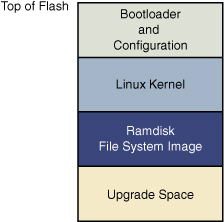
The bootloader is often placed in the top or bottom of the Flash memory array. Following the bootloader, space is allocated for the Linux kernel image and the ramdisk file system image,10 which holds the root file system. Typically, the Linux kernel and ramdisk file system images are compressed, and the bootloader handles the decompression task during the boot cycle.
For dynamic data that needs to be saved between reboots and power cycles, another small area of Flash can be dedicated, or another type of nonvolatile storage11 can be used. This is a typical configuration for embedded systems that have requirements to store configuration data, as might be found in a wireless access point aimed at the consumer market, for example.
2.3.4 Flash File Systems
The limitations of the simple Flash layout scheme just described can be overcome by using a Flash file system to manage data on the Flash device in a manner similar to how data is organized on a hard drive. Early implementations of file systems for Flash devices consisted of a simple block device layer that emulated the 512-byte sector layout of a common hard drive. These simple emulation layers allowed access to data in file format rather than unformatted bulk storage, but they had some performance limitations.
One of the first enhancements to Flash file systems was the incorporation of wear leveling. As discussed earlier, Flash blocks are subject to a finite write lifetime. Wear-leveling algorithms are used to distribute writes evenly over the physical erase blocks of the Flash memory in order to extend the life of the Flash memory chip.
Another limitation that arises from the Flash architecture is the risk of data loss during a power failure or premature shutdown. Consider that the Flash block sizes are relatively large and that average file sizes being written are often much smaller relative to the block size. You learned previously that Flash blocks must be written one block at a time. Therefore, to write a small 8KB file, you must erase and rewrite an entire Flash block, perhaps 64KB or 128KB in size; in the worst case, this can take several seconds to complete. This opens a significant window to risk of data loss due to power failure.
One of the more popular Flash file systems in use today is JFFS2, or Journaling Flash File System 2. It has several important features aimed at improving overall performance, increasing Flash lifetime, and reducing the risk of data loss in the case of power failure. The more significant improvements in the latest JFFS2 file system include improved wear leveling, compression and decompression to squeeze more data into a given Flash size, and support for Linux hard links. This topic is covered in detail in Chapter 9 and in Chapter 10, “MTD Subsystem,” when we discuss the Memory Technology Device (MTD) subsystem.
2.3.5 Memory Space
Virtually all legacy embedded operating systems view and manage system memory as a single large, flat address space. That is, a microprocessor’s address space exists from 0 to the top of its physical address range. For example, if a microprocessor had 24 physical address lines, its top of memory would be 16MB. Therefore, its hexadecimal address would range from 0x00000000 to 0x00ffffff. Hardware designs commonly place DRAM starting at the bottom of the range, and Flash memory from the top down. Unused address ranges between the top of DRAM and bottom of Flash would be allocated for addressing of various peripheral chips on the board. This design approach is often dictated by the choice of microprocessor. Figure 2-5 shows a typical memory layout for a simple embedded system.
Figure 2-5. Typical embedded system memory map

In traditional embedded systems based on legacy operating systems, the OS and all the tasks12 had equal access rights to all resources in the system. A bug in one process could wipe out memory contents anywhere in the system, whether it belonged to itself, the OS, another task, or even a hardware register somewhere in the address space. Although this approach had simplicity as its most valuable characteristic, it led to bugs that could be challenging to diagnose.
High-performance microprocessors contain complex hardware engines called Memory Management Units (MMUs). Their purpose is to enable an operating system to exercise a high degree of management and control over its address space and the address space it allocates to processes. This control comes in two primary forms: access rights and memory translation. Access rights allow an operating system to assign specific memory-access privileges to specific tasks. Memory translation allows an operating system to virtualize its address space, which has many benefits.
The Linux kernel takes advantage of these hardware MMUs to create a virtual memory operating system. One of the biggest benefits of virtual memory is that it can make more efficient use of physical memory by presenting the appearance that the system has more memory than is physically present. The other benefit is that the kernel can enforce access rights to each range of system memory that it allocates to a task or process, to prevent one process from errantly accessing memory or other resources that belong to another process or to the kernel itself.
The next section examines in more detail how this works. A tutorial on the complexities of virtual memory systems is beyond the scope of this book.13 Instead, we examine the ramifications of a virtual memory system as it appears to an embedded systems developer.
2.3.6 Execution Contexts
One of the very first chores that Linux performs is to configure the hardware MMU on the processor and the data structures used to support it, and to enable address translation. When this step is complete, the kernel runs in its own virtual memory space. The virtual kernel address selected by the kernel developers in recent Linux kernel versions defaults to 0xC0000000. In most architectures, this is a configurable parameter.14 If we looked at the kernel’s symbol table, we would find kernel symbols linked at an address starting with 0xC0xxxxxx. As a result, any time the kernel executes code in kernel space, the processor’s instruction pointer (program counter) contains values in this range.
In Linux, we refer to two distinctly separate operational contexts, based on the environment in which a given thread15 is executing. Threads executing entirely within the kernel are said to be operating in kernel context. Application programs are said to operate in user space context. A user space process can access only memory it owns, and it is required to use kernel system calls to access privileged resources such as file and device I/O. An example might make this more clear.
Consider an application that opens a file and issues a read request, as shown in Figure 2-6. The read function call begins in user space, in the C library read() function. The C library then issues a read request to the kernel. The read request results in a context switch from the user’s program to the kernel, to service the request for the file’s data. Inside the kernel, the read request results in a hard-drive access requesting the sectors containing the file’s data.
Figure 2-6. Simple file read request
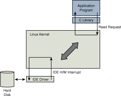
Usually the hard-drive read request is issued asynchronously to the hardware itself. That is, the request is posted to the hardware, and when the data is ready, the hardware interrupts the processor. The application program waiting for the data is blocked on a wait queue until the data is available. Later, when the hard disk has the data ready, it posts a hardware interrupt. (This description is intentionally simplified for the purposes of this illustration.) When the kernel receives the hardware interrupt, it suspends whatever process was executing and proceeds to read the waiting data from the drive.
To summarize this discussion, we have identified two general execution contexts—user space and kernel space. When an application program executes a system call that results in a context switch and enters the kernel, it is executing kernel code on behalf of a process. You will often hear this referred to as process context within the kernel. In contrast, the interrupt service routine (ISR) handling the IDE drive (or any other ISR, for that matter) is kernel code that is not executing on behalf of any particular process. This is typically called interrupt context.
Several limitations exist in this operational context, including the limitation that the ISR cannot block (sleep) or call any kernel functions that might result in blocking. For further reading on these concepts, consult the references at the end of this chapter.
2.3.7 Process Virtual Memory
When a process is spawned—for example, when the user types ls at the Linux command prompt—the kernel allocates memory for the process and assigns a range of virtual-memory addresses to the process. The resulting address values bear no fixed relationship to those in the kernel, nor to any other running process. Furthermore, there is no direct correlation between the physical memory addresses on the board and the virtual memory as seen by the process. In fact, it is not uncommon for a process to occupy multiple different physical addresses in main memory during its lifetime as a result of paging and swapping.
Listing 2-4 is the venerable “Hello World,” modified to illustrate the concepts just discussed. The goal of this example is to illustrate the address space that the kernel assigns to the process. This code was compiled and run on an embedded system containing 256MB of DRAM memory.
Listing 2-4. Hello World, Embedded Style
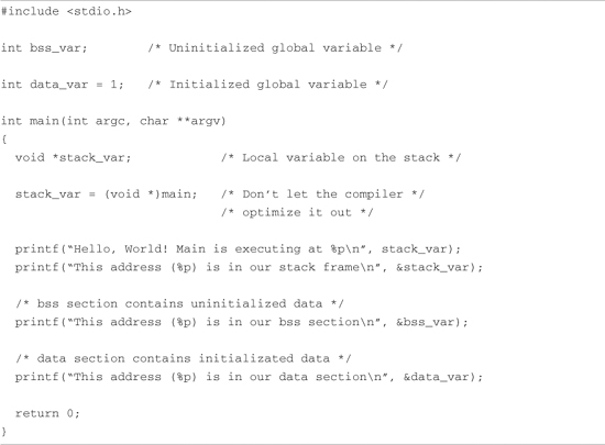
Listing 2-5 shows the console output that this program produces. Notice that the process called hello thinks it is executing somewhere in high RAM just above the 256MB boundary (0x10000418). Notice also that the stack address is roughly halfway into a 32-bit address space, well beyond our 256MB of RAM (0x7ff8ebb0). How can this be? DRAM is usually contiguous in systems like these. To the casual observer, it appears that we have nearly 2GB of DRAM available for our use. These virtual addresses were assigned by the kernel and are backed by physical RAM somewhere within the 256MB range of available memory on our embedded board.
Listing 2-5. Hello Output

One of the characteristics of a virtual memory system is that when available physical RAM goes below a designated threshold, the kernel can swap out memory pages to a bulk storage medium, usually a hard disk drive (if available). The kernel examines its active memory regions, determines which areas in memory have been least recently used, and swaps out these memory regions to disk to free them for the current process. Developers of embedded systems often disable swapping on embedded systems because of performance or resource constraints. For example, it would be ridiculous in most cases to use a relatively slow Flash memory device with limited write life cycles as a swap device. Without a swap device, you must carefully design your applications to exist within the limitations of your available physical memory.
2.3.8 Cross-Development Environment
Before we can develop applications and device drivers for an embedded system, we need a set of tools (compiler, utilities, and so on) that will generate binary executables in the proper format for the target system. Consider a simple application written on your desktop PC, such as the traditional “Hello World” example. After you have created the source code on your desktop, you invoke the compiler that came with your desktop system (usually GNU gcc) to generate a binary executable image. That image file is properly formatted to execute on the machine on which it was compiled. This is referred to as native compilation. In other words, using compilers on your desktop system, you generate code that will execute on that desktop system.
Note that native does not imply an architecture. Indeed, if you have a toolchain that runs on your target board, you can natively compile applications for your target’s architecture. In fact, one great way to stress-test a new embedded kernel and custom board is to repeatedly compile the Linux kernel on it.
Developing software in a cross-development environment requires that the compiler running on your development host output a binary executable that is incompatible with the desktop development workstation on which it was compiled. The primary reason these tools exist is that it is often impractical or impossible to develop and compile software natively on the embedded system because of resource (typically memory and CPU horsepower) constraints.
Numerous hidden traps to this approach often catch the unwary newcomer to embedded development. When a given program is compiled, the compiler often knows how to find include files, and where to find libraries that might be required for the compilation to succeed. To illustrate these concepts, let’s look again at the “Hello World” program. The example reproduced in Listing 2-4 was compiled with the following command line:
gcc -Wall -o hello hello.c
In Listing 2-4, we see an include file, stdio.h. This file does not reside in the same directory as the hello.c file specified on the gcc command line. So how does the compiler find them? Also, the printf() function is not defined in the file hello.c. Therefore, when hello.c is compiled, it will contain an unresolved reference for this symbol. How does the linker resolve this reference at link time?
Compilers have built-in defaults for locating include files. When the reference to the include file is encountered, the compiler searches its default list of locations to find the file. A similar process exists for the linker to resolve the reference to the external symbol printf(). The linker knows by default to search the C library (libc-*) for unresolved references, and it knows where to find the reference on your system. Again, this default behavior is built into the toolchain.
Now assume you are building an application targeting a Power Architecture embedded system. Obviously, you will need a cross-compiler to generate binary executables compatible with the Power Architecture processor. If you issue a similar compilation command using your cross-compiler to compile the preceding hello.c example, it is possible that your binary executable could end up being accidentally linked with an x86 version of the C library on your development system, attempting to resolve the reference to printf(). Of course, the results of running this bogus hybrid executable, containing a mix of Power Architecture and x86 binary instructions,16 are predictable: crash!
The solution to this predicament is to instruct the cross-compiler to look in nonstandard locations to pick up the header files and target specific libraries. We cover this topic in much more detail in Chapter 12. The intent of this example was to illustrate the differences between a native development environment and a development environment targeted at cross-compilation for embedded systems. This is but one of the complexities of a cross-development environment. The same issue and solutions apply to cross-debugging, as you will see starting in Chapter 14, “Kernel Debugging Techniques.” A proper cross-development environment is crucial to your success and involves much more than just compilers, as you will see in Chapter 12.
2.4 Embedded Linux Distributions
What exactly is a Linux distribution? After the Linux kernel boots, it expects to find and mount a root file system. When a suitable root file system has been mounted, startup scripts launch a number of programs and utilities that the system requires. These programs often invoke other programs to do specific tasks, such as spawn a login shell, initialize network interfaces, and launch a user’s applications. Each of these programs has specific requirements (often called dependencies) that must be satisfied by other components in the system. Most Linux application programs depend on one or more system libraries. Other programs require configuration and log files, and so on. In summary, even a small embedded Linux system needs many dozens of files populated in an appropriate directory structure on a root file system.
Full-blown desktop systems have many thousands of files on the root file system. These files come from packages that are usually grouped by functionality. The packages typically are installed and managed using a package manager. Red Hat’s Package Manager (rpm) is a popular example and is widely used to install, remove, and update packages on a Linux system. If your Linux workstation is based on Red Hat, including the Fedora series, typing rpm -qa at a command prompt lists all the packages installed on your system. If you are using a distribution based on Debian, such as Ubuntu, typing dpkg -l has the same result.
A package can consist of many files; indeed, some packages contain hundreds of files. A complete Linux distribution can contain hundreds or even thousands of packages. These are some examples of packages you might find on an embedded Linux distribution, and their purpose:
• initscripts contains basic system startup and shutdown scripts.
• apache implements the popular Apache web server.
• telnet-server contains files necessary to implement telnet server functionality, which allows you to establish telnet sessions to your embedded target.
• glibc implements the Standard C library.
• busybox contains compact versions of dozens of popular command-line utilities commonly found on UNIX/Linux systems.17
This is the purpose of a Linux distribution, as the term has come to be used. A typical Linux distribution comes with several CD-ROMs full of useful programs, libraries, tools, utilities, and documentation. Installation of a distribution typically leaves the user with a fully functional system based on a reasonable set of default configuration options, which can be tailored to suit a particular set of requirements. You may be familiar with one of the popular desktop Linux distributions, such as Red Hat or Ubuntu.
A Linux distribution for embedded targets differs in several significant ways. First, the executable target binaries from an embedded distribution will not run on your PC, but are targeted to the architecture and processor of your embedded system. (Of course, if your embedded Linux distribution targets the x86 architecture, this statement does not necessarily apply.) A desktop Linux distribution tends to have many GUI tools aimed at the typical desktop user, such as fancy graphical clocks, calculators, personal time-management tools, e-mail clients, and more. An embedded Linux distribution typically omits these components in favor of specialized tools aimed at developers, such as memory analysis tools, remote debug facilities, and many more.
Another significant difference between desktop and embedded Linux distributions is that an embedded distribution typically contains cross tools, as opposed to native tools. For example, the gcc toolchain that ships with an embedded Linux distribution runs on your x86 desktop PC but produces binary code that runs on your target system, often a non-x86 architecture. Many of the other tools in the toolchain are similarly configured: They run on the development host (usually an x86 PC) but are designed to emit or manipulate objects targeted at foreign architectures such as ARM or Power Architecture.
2.4.1 Commercial Linux Distributions
Several vendors of commercial embedded Linux distributions exist. The leading embedded Linux vendors have been shipping embedded Linux distributions for years. It is relatively easy to find information on the leading embedded Linux vendors. A quick Internet search for “embedded Linux distributions” points to several compilations. One particularly good compilation can be found at http://elinux.org/Embedded_Linux_Distributions.
2.4.2 Do-It-Yourself Linux Distributions
You can choose to assemble all the components you need for your embedded project on your own. You have to decide whether the risks are worth the effort. If you find yourself involved with embedded Linux purely for the pleasure of it, such as for a hobby or college project, this approach might be a good one. However, plan to spend a significant amount of time assembling all the tools and utilities your project needs and making sure they all interoperate.
For starters, you need a toolchain. gcc and binutils are available from www.fsf.org and other mirrors around the world. Both are required to compile the kernel and user-space applications for your project. These are distributed primarily in source code form, and you must compile the tools to suit your particular cross-development environment. Patches are often required to the most recent “stable” source trees of these utilities, especially when they will be used beyond the x86/IA32 architecture. The patches usually can be found at the same location as the base packages. The challenge is to discover which collections of patches you need for your particular problem or architecture.
As soon as your toolchain is working, you need to download and compile many application packages along with the dependencies they require. This can be a formidable challenge, since many packages even today do not lend themselves to cross-compiling. Many still have build or other issues when moved away from their native x86 environment where they were developed.
Beyond these challenges, you might want to assemble a competent development environment, containing tools such as graphical debuggers, memory analysis tools, system tracing and profiling tools, and more. You can see from this discussion that building your own embedded Linux distribution can be quite challenging.
2.5 Summary
This chapter covered many subjects in a broad fashion. Now you have a proper perspective for the material to follow. In later chapters, this perspective will be expanded to help you develop the skills and knowledge required to be successful in your next embedded project.
• Embedded systems share some common attributes. Often resources are limited, and user interfaces are simple or nonexistent and are often designed for a specific purpose.
• The bootloader is a critical component of a typical embedded system. If your embedded system is based on a custom-designed board, you must provide a bootloader as part of your design. Often this is just a porting effort of an existing bootloader.
• Several software components are required to boot a custom board, including the bootloader and the kernel and file system image.
• Flash memory is widely used as a storage medium in embedded Linux systems. This chapter introduced the concept of Flash memory. Chapters 9 and 10 expand on this coverage.
• An application program, also called a process, lives in its own virtual memory space assigned by the kernel. Application programs are said to run in user space.
• A properly equipped and configured cross-development environment is crucial to the embedded developer. Chapter 12 is devoted to this important subject.
• You need an embedded Linux distribution to begin developing your embedded target. Embedded distributions contain many components, compiled and optimized for your chosen architecture.
2.5.1 Suggestions for Additional Reading
Linux Kernel Development, 3rd Edition
Robert Love
Addison-Wesley, 2010
Understanding the Linux Kernel
Daniel P. Bovet and Marco Cesati
O’Reilly & Associates, Inc., 2002
Understanding the Linux Virtual Memory Manager
Bruce Perens
Prentice Hall, 2004