
Chapter 9. File Systems
Perhaps one of the most important decisions an embedded developer makes is which file system(s) to deploy. Some file systems optimize for performance, whereas others optimize for size. Still others optimize for data recovery after device or power failure. This chapter introduces the major file systems in use on Linux systems and examines the characteristics of each as they apply to embedded designs. It is not the intent of this chapter to examine the internal technical details of each file system. Instead, this chapter examines the operational characteristics and development issues related to each file system presented.
Starting with the most popular file system in use on earlier Linux desktop distributions, we introduce concepts from the Second Extended File System (ext2) to lay a foundation for further discussion. Next we look at its successor, the Third Extended File System (ext3), which has enjoyed much popularity as the default file system for many Linux desktop and server distributions. We then describe the improvements that led to ext4.
After introducing some fundamentals, we examine a variety of specialized file systems, including those optimized for data recovery and storage space, and those designed for use on Flash memory devices. The Network File System (NFS) is presented, followed by a discussion of the more important pseudo file systems, including the /proc file system and sysfs.
9.1 Linux File System Concepts
Before delving into the details of the individual file systems, let’s look at the big picture of how data is stored on a Linux system. In our study of device drivers in Chapter 8, “Device Driver Basics,” we looked at the structure of a character device. In general, character devices store and retrieve data in serial streams. The most basic example of a character device is a serial port or mouse. In contrast, block devices store and retrieve data in equal-sized chunks of data at a time, in random locations on an addressable medium. For example, a typical IDE hard disk controller can transfer 512 bytes of data at a time to and from a specific, addressable location on the physical medium.
9.1.1 Partitions
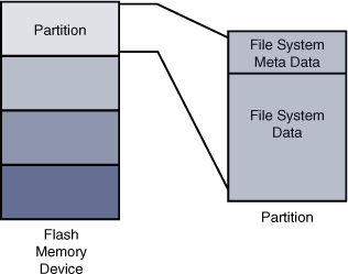
Before we begin our discussion of file systems, we start by introducing partitions, the logical division of a physical device on which a file system exists. At the highest level, data is stored on physical devices in partitions. A partition is a logical division of the physical medium (hard disk, Flash memory) whose data is organized following the specifications of a given partition type. A physical device can have a single partition covering all its available space, or it can be divided into multiple partitions to suit a particular task. A partition can be thought of as a logical disk onto which a complete file system can be written.
Figure 9-1 shows the relationship between partitions and file systems.
Figure 9-1. Partitions and file systems
Linux uses a utility called fdisk to manipulate partitions on block devices. A recent fdisk utility found on many Linux distributions has knowledge of more than 90 different partition types. In practice, only a few are commonly used on Linux systems. Some common partition types are Linux, FAT32, and Linux Swap.
Listing 9-1 displays the output of the fdisk utility targeting a CompactFlash device connected to a USB port. On this particular target system, the physical CompactFlash device was assigned to the device node /dev/sdb.1
Listing 9-1. Displaying Partition Information Using fdisk
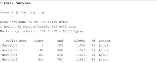
For this discussion, we have created four partitions on the device using the fdisk utility. One of them is marked bootable, as indicated by the asterisk in the Boot column. This reflects a boot indicator flag in the data structure that represents the partition table on the device. As you can see from the listing, the logical unit of storage used by fdisk is a cylinder.2 On this device, a cylinder contains 64KB. On the other hand, Linux represents the smallest unit of storage as a logical block. You can deduce from this listing that a block is a unit of 1024 bytes.
After the CompactFlash has been partitioned in this manner, each device representing a partition can be formatted with the file system of your choice. When a partition is formatted with a given file system type, Linux can mount the corresponding file system from that partition.
9.2 ext2
Building on Listing 9-1, we need to format the partitions created with fdisk. To do so, we use the Linux mkfs.ext2 utility. mkfs.ext2 is similar to the familiar DOS format command. This utility makes a file system of type ext2 on the specified partition. mkfs.ext2 is specific to the ext2 file system; other file systems have their own versions of these utilities. Listing 9-2 captures the output of this process.
Listing 9-2. Formatting a Partition Using mkfs.ext2
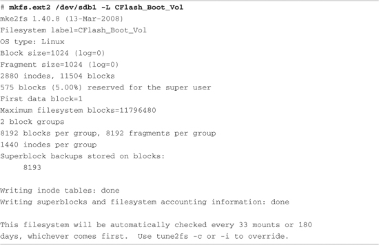
Listing 9-2 contains much detail relating to the ext2 file system. It’s an excellent way to begin understanding the operational characteristics of ext2. This partition was formatted as type ext2 (we know this because we used the ext2 mkfs utility) with a volume label of CFlash_Boot_Vol. It was created on a Linux partition (OS Type:) with a block size of 1024 bytes. Space was allocated for 2,880 inodes, occupying 11,504 blocks. An inode is the fundamental data structure representing a single file. For more detailed information about the internal structure of the ext2 file system, see the last section of this chapter.
Looking at the output of mkfs.ext2 in Listing 9-2, we can ascertain certain characteristics of how the storage device is organized. We already know that the block size is 1024 bytes. If necessary for your particular application, mkfs.ext2 can be instructed to format an ext2 file system with different block sizes. Current implementations allow block sizes of 1,024, 2,048, and 4,096 blocks.
Block size is always a compromise for best performance. On one hand, large block sizes waste more space on disks with many small files, because each file must fit into an integral number of blocks. Any leftover fragment above block_size * n must occupy another full block, even if only 1 byte. On the other hand, very small block sizes increase the file system overhead of managing the metadata that describes the block-to-file mapping. Benchmark testing on your particular hardware implementation and data formats is the only way to be sure you have selected an optimum block size.
9.2.1 Mounting a File System
After a file system has been created, we can mount it on a running Linux system. The kernel must be compiled with support for our particular file system type, either as a compiled-in module or as a dynamically loadable module. The following command mounts the previously created ext2 file system on a mount point that we specify:
# mount /dev/sdb1 /mnt/flash
This example assumes that we have a directory created on our target Linux machine called /mnt/flash. This is called the mount point because we are installing (mounting) the file system rooted at this point in our file system hierarchy. We are mounting the Flash device described earlier that was assigned to the device /dev/sdb1. On a typical Linux desktop (development) machine, we need to have root privileges to execute this command.3 The mount point is any directory path on your file system that you decide, which becomes the top level (root) of your newly mounted device. In the preceding example, to reference any files on your Flash device, you must prefix the path with /mnt/flash.
The mount command has many options. Several options that mount accepts depend on the target file system type. Most of the time, mount can determine the type of file system on a properly formatted file system known to the kernel. We’ll provide additional usage examples for the mount command as we proceed through this chapter.
Listing 9-3 displays the directory contents of a Flash device configured for an arbitrary embedded system.
Listing 9-3. Flash Device Listing

Listing 9-3 is an example of what an embedded system’s root file system might look like at the top (root) level. Chapter 6, “User Space Initialization,” provides guidance on and examples of how to determine the contents of the root file system.
9.2.2 Checking File System Integrity
The e2fsck command is used to check the integrity of an ext2 file system. A file system can become corrupted for several reasons. By far the most common reason is an unexpected power failure. Linux distributions close all open files and unmount file systems during the shutdown sequence (assuming an orderly shutdown of the system). However, when we are dealing with embedded systems, unexpected power-downs are common, so we need to provide some defensive measures against these cases. e2fsck is our first line of defense.
Listing 9-4 shows the output of e2fsck run on our CompactFlash from the previous examples. It has been formatted and properly unmounted, so no errors should occur.
Listing 9-4. Clean File System Check

The e2fsck utility checks several aspects of the file system for consistency. If no issues are found, e2fsck issues a message similar to that shown in Listing 9-4. Note that e2fsck should be run only on an unmounted file system. Although it is possible to run it on a mounted file system, doing so can cause significant damage to internal file system structures on the disk or Flash device.
To offer a more interesting example, Listing 9-5 was created by pulling the CompactFlash device out of its socket while it was still mounted. We intentionally created a file and started an editing session on that file before removing it from the system. This can result in corruption of the data structures describing the file, as well as the actual data blocks containing the file’s data.
Listing 9-5. Corrupted File System Check

From Listing 9-5, you can see that e2fsck detected that the CompactFlash was not cleanly unmounted. Furthermore, you can see the processing on the file system during e2fsck checking. The e2fsck utility makes five passes over the file system, checking various elements of the internal file system’s data structures. An error associated with a file, identified by inode4 13, was automatically fixed because the -y flag was included on the e2fsck command line.
Of course, in a real system, you might not be this lucky. Some types of file system errors cannot be repaired using e2fsck. Moreover, the embedded system designer should understand that if power has been removed without proper shutdown, the boot cycle can be delayed by the length of time it takes to scan your boot device and repair any errors. Indeed, if these errors are not repairable, the system boot is halted, and manual intervention is indicated. Furthermore, it should be noted that if your file system is large, the file system check (fsck) can take minutes or even hours for large multigigabyte file systems.
Another defense against file system corruption is to ensure that writes are committed to disk immediately when written. The sync utility can be used to force all queued I/O requests to be committed to their respective devices. One strategy to minimize the window of vulnerability for data corruption from unexpected power loss or drive failure is to issue the sync command after every file write or strategically as needed by your application requirements. The trade-off is, of course, a performance penalty. Deferring disk writes is a performance optimization used in all modern operating systems. Using sync effectively defeats this optimization.
The ext2 file system has matured as a fast, efficient, and robust file system for Linux systems. However, if you need the additional reliability of a journaling file system, or if boot time after unclean shutdown is an issue in your design, you should consider the ext3 file system.
9.3 ext3
The ext3 file system has become a powerful, high-performance, and robust journaling file system. It is currently the default file system for many popular desktop Linux distributions.
The ext3 file system is basically an extension of the ext2 file system with added journaling capability. Journaling is a technique in which each change to the file system is logged in a special file so that recovery is possible from known journaling points. One of the primary advantages of the ext3 file system is its ability to be mounted directly after an unclean shutdown. As stated in the preceding section, when a system shuts down unexpectedly, such as during a power failure, the system forces a file system consistency check, which can be a lengthy operation. With ext3 file systems, a consistency check is unneeded, because the journal can simply be played back to ensure the file system’s consistency.
Without going into design details that are beyond the scope of this book, we will quickly explain how a journaling file system works. A journaling file system contains a special file, often hidden from the user, that is used to store file system metadata5 and file data itself. This special file is referred to as the journal. Whenever the file system is subject to a change (such as a write operation), the changes are first written to the journal. The file system drivers make sure that this write is committed to the journal before the actual changes are posted and committed to the storage medium (disk or Flash, for example). After the changes have been logged in the journal, the driver posts the changes to the actual file and metadata on the medium. If a power failure occurs during the media write and a reboot occurs, all that is necessary to restore consistency to the file system is to replay the changes in the journal.
One of the most significant design goals for the ext3 file system was that it be both backward- and forward-compatible with the ext2 file system. It is possible to convert an ext2 file system to an ext3 file system and back again without reformatting or rewriting all the data on the disk. Let’s see how this is done.6 Listing 9-6 details the procedure.
Listing 9-6. Converting an ext2 File System to an ext3 File System
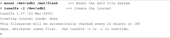
Notice that first we mounted the file system on /mnt/flash for illustrative purposes only. Normally, we would execute this command on an unmounted ext2 partition. The design behavior for tune2fs when the file system is mounted is to create the journal file called .journal, a hidden file. A file in Linux preceded by a period (.) is considered a hidden file; most Linux command-line file utilities silently ignore files of this type. In Listing 9-7, we can see that the ls command is invoked with the -a flag, which tells the ls utility to list all files.
Listing 9-7. ext3 Journal File
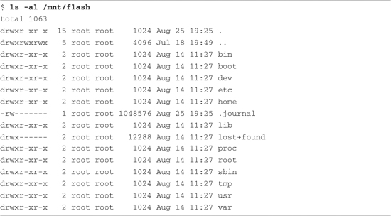
Now that we have created the journal file on our Flash module, it is effectively formatted as an ext3 file system. The next time the system is rebooted or the e2fsck utility is run on the partition containing the newly created ext3 file system, the journal file is automatically made invisible. Its metadata is stored in a reserved inode set aside for this purpose. As long as the .journal file is visible in the directory listing, it is dangerous to modify or delete this file.
It is possible and sometimes advantageous to create the journal file on a different device. For example, if your system has more than one physical device, you can place your ext3 journaling file system on the first drive and have the journal file on the second drive. This method works regardless of whether your physical storage is based on Flash or rotational media. To create the journaling file system from an existing ext2 file system with the journal file in a separate partition, invoke tune2fs in the following manner:
# tune2fs -J device=/dev/sda1 -j /dev/sdb1
For this to work, you must have already formatted the device where the journal is to reside with a journal file—it must be an ext3 file system.
9.4 ext4
The ext4 file system builds on the success of the ext3 file system. Like its predecessor, it is a journaling file system. It was developed as a series of patches designed to remove some of the limitations of the ext3 file system. It is likely that ext4 will become the default file system for a number of popular Linux distributions.
The ext4 file system removed the 16-terabyte limit for file systems, increasing the size to 1 exbibyte (260 bytes, if you can count that high!) and supports individual file sizes up to 1024 gigabytes. (I can’t pronounce exbibyte, much less comprehend that quantity!) Several other improvements have been made to increase performance for the types of loads expected on large server and database systems, where ext4 is expected to be the default.
If your embedded system requirements include support for large, high-performance journaling file systems, you might consider investigating ext4.
9.5 ReiserFS
The ReiserFS file system has enjoyed popularity among some desktop distributions such as SuSE and Gentoo. Reiser4 is the current incarnation of this journaling file system. Like the ext3 file system, ReiserFS guarantees that either a given file system operation completes in its entirety, or none of it completes. Unlike ext3, Reiser4 has introduced an API for system programmers to guarantee the atomicity of a file system transaction. Consider the following example:
A database program is busy updating records in the database. Several writes are issued to the file system. Power is lost after the first write but before the last one has completed. A journaling file system guarantees that the metadata changes have been stored to the journal file so that when power is again applied to the system, the kernel can at least establish a consistent state of the file system. That is, if file A was reported as having 16KB before the power failure, it will be reported as having 16KB afterward, and the directory entry representing this file (actually, the inode) properly records the file’s size. This does not mean, however, that the file data was properly written to the file; it indicates only that there are no errors on the file system. Indeed, it is likely that data was lost by the database program in the previous scenario, and it would be up to the database logic to recover the lost if, in fact, recovery is even possible.
Reiser4 implements high-performance “atomic” file system operations designed to protect both the state of the file system (its consistency) and the data involved in a file system operation. Reiser4 provides a user-level API to enable programs such as database managers to issue a file system write command that is guaranteed to either succeed in its entirety or fail in a similar manner. This guarantees not only that file system consistency is maintained, but also that no partial data or garbage data remains in files after a system crash.
For more details and the actual software for ReiserFS, consult the references at the end of this chapter.
9.6 JFFS2
Flash memory has been used extensively in embedded products. Because of the nature of Flash memory technology, it is inherently less efficient and more prone to data corruption caused by power loss. This is due to much larger write times. The inefficiency stems from the block size. Block sizes of Flash memory devices are often measured in the tens or hundreds of kilobytes. Flash memory can be erased only a block at a time, although writes usually can be executed 1 byte or word at a time. To update a single file, an entire block must be erased and rewritten.
It is well known that the distribution of file sizes on any given Linux machine (or other OS) contains many more smaller files than larger files. The histogram shown in Figure 9-2, generated with gnuplot, illustrates the distribution of file sizes on a typical Linux development system.
Figure 9-2. File sizes in bytes
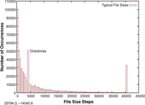
Figure 9-2 shows that the majority of file sizes are well below approximately 5KB. The spike at 4096 represents directories. Directory entries (also files themselves) are exactly 4096 bytes in length, and there are many of them. The spike above 40,000 bytes is an artifact of the measurement. It is a count of the number of files greater than approximately 40KB, the end of the measurement quantum. It is interesting to note that the vast majority of files are very small.
Small file sizes present a unique challenge to the Flash file system designer. Because Flash memory must be erased an entire block at a time, and the size of a Flash block is often many multiples of the smaller file sizes, Flash is subject to time-consuming block rewriting operations. For example, assume that a 128KB block of Flash is being used to hold a couple dozen files of 4096 bytes or less. Now assume that one of those files needs to be modified. This causes the Flash file system to invalidate the entire 128KB block and rewrite every file in the block to a newly erased block. This can be a time-consuming process.
Because Flash writes can be time-consuming (much slower than hard disk writes), this increases the window where data corruption can occur due to a sudden loss of power. Unexpected power loss is a common occurrence in embedded systems. For instance, if power is lost during the rewrite of the 128KB data block just mentioned, all of the couple dozen files potentially could be lost.
Enter the second-generation Journaling Flash File System (JFFS2). The issues just discussed and other problems have been largely reduced or eliminated by the design of JFFS2. The original JFFS was designed by Axis Communications AB of Sweden and was targeted specifically at the commonly available Flash memory devices of the time. The JFFS had knowledge of the Flash architecture and, more important, architectural limitations imposed by the devices.
Another problem with Flash file systems is that Flash memory has a limited lifetime. Typical Flash memory devices are specified for a minimum of 100,000 write cycles, and, more recently, 1,000,000-cycle devices have become common. This specification is applicable to each block of the Flash device. This unusual limitation imposes the requirement to spread the writes evenly across the blocks of a Flash memory device. JFFS2 uses a technique called wear leveling to accomplish this function.
9.6.1 Building a JFFS2 Image
Building a JFFS2 image is relatively straightforward. Although you can build a JFFS2 image on your workstation without kernel support, you cannot mount it. Before proceeding, ensure that your kernel has support for JFFS2 and that your development workstation contains a compatible version of the mkfs.jffs2 utility. These utilities can be downloaded and built from source code, ftp://ftp.infradead.org/pub/mtd-utils/. Preferably, they should be available from your desktop Linux package maintainer. For example, on Ubuntu, they can be installed by executing this command:
$ sudo apt-get install mtd-tools
Your distribution may call them something different, such as mtd-utils. Consult the documentation that came with your desktop Linux distribution.
JFFS2 images are built from a directory that contains the desired files on the file system image. Listing 9-8 shows a typical directory structure for a Flash device designed to be used as a root file system.
Listing 9-8. Directory Layout for a JFFS2 File System
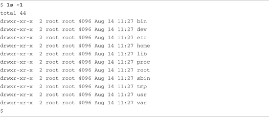
When suitably populated with runtime files, this directory layout can be used as a template for the mkfs.jffs2 command. The mkfs.jffs2 command produces a properly formatted JFFS2 file system image from a directory tree such as that shown in Listing 9-8. Command-line parameters are used to pass mkfs.jffs2 the directory location as well as the name of the output file to receive the JFFS2 image. The default is to create the JFFS2 image from the current directory. Listing 9-9 shows the command for building the JFFS2 image.
Listing 9-9. mkfs.jffs2 Command Example
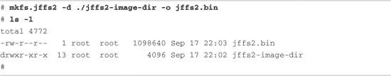
The directory structure and files from Listing 9-8 are in the jffs2-image-dir directory in our example. We arbitrarily execute the mkfs.jffs2 command from the directory above our file system image. Using the -d flag, we tell the mkfs.jffs2 command where the file system template is located. We use the -o flag to name the output file to which the resulting JFFS2 image is written. The resulting image, jffs2.bin, is used in Chapter 10, “MTD Subsystem,” when we examine the JFFS2 file together with the MTD subsystem.
It should be pointed out that any Flash-based file system that supports write operations is subject to conditions that can lead to premature failure of the underlying Flash device. For example, enabling system loggers (syslogd and klogd) configured to write their data to Flash-based file systems can easily overwhelm a Flash device with continuous writes. Some categories of program errors can also lead to continuous writes. Care must be taken to limit Flash writes to values within the lifetime of Flash devices.
9.7 cramfs
From the README file in the cramfs project, the goal of cramfs is to “cram a file system into a small ROM.” The cramfs file system is very useful for embedded systems that contain a small ROM or FLASH memory that holds static data and programs. Borrowing again from the cramfs README file, “cramfs is designed to be simple and small, and compress things well.”
The cramfs file system is read-only. It is created with a command-line utility called mkcramfs. If you don’t have it on your development workstation, you can download it from the URL provided at the end of this chapter. As with JFFS2, mkcramfs builds a file system image from a directory specified on the command line. Listing 9-10 details the procedure for building a cramfs image. We use the same file system structure from Listing 9-8 that we used to build the JFFS2 image.
Listing 9-10. mkcramfs Command Example

The mkcramfs command was initially issued without any command-line parameters to reproduce the usage message. Because this utility has no man page, this is the best way to understand its usage. We subsequently issued the command specifying the current directory (.) as the source of the files for the cramfs file system, and a file called cramfs.image as the destination. Finally, we listed the file just created, and we see a new file called cramfs.image.
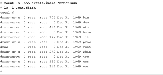
Note that if your kernel is configured with cramfs support, you can mount this file system image on your Linux development workstation and examine its contents. Of course, because it is a read-only file system, you cannot modify it. Listing 9-11 demonstrates mounting the cramfs file system on a mount point called /mnt/flash.
Listing 9-11. Examining the cramfs File System
You might have noticed the warning message regarding group ID (GID) in Listing 9-10 when the mkcramfs command was executed. The cramfs file system uses very terse metadata to reduce file system size and increase the speed of execution. One of the “features” of the cramfs file system is that it truncates the group ID field to 8 bits. Linux uses the 16-bit group ID field. The result is that files created with group IDs greater than 255 are truncated with the warning issued in Listing 9-10.
Although somewhat limited in terms of maximum file sizes, maximum number of files, and so on, the cramfs file system is ideal for boot ROMs, in which read-only operation and fast compression are desirable features.
9.8 Network File System
If you have developed in the UNIX environment, you undoubtedly are familiar with the Network File System (NFS). Properly configured, NFS enables you to export a directory on an NFS server and mount that directory on a remote client machine as if it were a local file system. This is useful in general for large networks of UNIX/Linux machines, and it can be a panacea to the embedded developer. Using NFS on your target board, an embedded developer can have access to a huge number of files, libraries, tools, and utilities during development and debugging, even if the target embedded system is resource-constrained.
As with the other file systems, your kernel must be configured with NFS support, for both the server-side functionality and the client side. NFS server and client functionality is independently configured in the kernel configuration.
Detailed instructions for configuring and tuning NFS are beyond the scope of this book, but a short introduction will help illustrate how useful NFS can be during development in the embedded environment. See the section at the end of this chapter for a pointer to detailed information about NFS, including the complete NFS Howto.
On your development workstation with NFS enabled, a configuration file contains a list specifying each directory that you want to export via the Network File System. On Red Hat, Ubuntu, and most other distributions, this file is located in the /etc directory and is named exports. Listing 9-12 is a sample /etc/exports, such as might be found on a development workstation used for embedded development.
Listing 9-12. Contents of /etc/exports

This file contains the names of two directories on a Linux development workstation. The first directory contains a target file system for an ADI Engineering Coyote reference board. The second directory is a general workspace that contains projects targeted for an embedded system. This is arbitrary; you can configure NFS any way you choose.
On an embedded system with NFS enabled, the following command mounts the .../workspace directory exported by the NFS server on a mount point of our choosing:
# mount -t nfs pluto:/home/chris/workspace /workspace
Notice some important points about this command. We are instructing the mount command to mount a remote directory (on a machine named pluto, our development workstation in this example) onto a local mount point called /workspace. For the command semantics to work, two requirements must be met on the embedded target. First, for the target to recognize the symbolic machine name pluto, it must be able to resolve the symbolic name. The easiest way to do this is to place an entry in the /etc/hosts file on the target. This allows the networking subsystem to resolve the symbolic name to its corresponding IP address. The entry in the target’s /etc/hosts file would look like this:
192.168.11.9 pluto
The second requirement is that the embedded target must have a directory in its root directory called /workspace. (You may choose any pathname you wish. For example, you could mount it on /mnt/mywork.) This is called a mount point. The requirement is that the target must have a directory created with the same name as given on the mount command.
The mount command in the preceding example causes the contents of the NFS server’s /home/chris/workspace directory to be available on the embedded system’s /workspace path.
This is quite useful, especially in a cross-development environment. Let’s say that you are working on a large project for your embedded device. Each time you make changes to the project, you need to move that application to your target so that you can test and debug it. Using NFS in the manner just described, assuming that you are working in the NFS exported directory on your host, the changes are immediately available on your target embedded system without the need to upload the newly compiled project files. This can speed development considerably.
9.8.1 Root File System on NFS
Mounting your project workspace on your target embedded system is very useful for development and debugging because it facilitates rapid access to changes and source code for source-level debugging. This is especially useful when the target system is severely resource-constrained. NFS really shines as a development tool when you mount your embedded system’s root file system entirely from an NFS server. In Listing 9-12, notice the coyote-target entry. This directory on your development workstation could contain hundreds or thousands of files compatible with your target architecture.
The leading embedded Linux distributions targeted at embedded systems ship tens of thousands of files compiled and tested for the chosen target architecture. To illustrate this, Listing 9-13 contains a directory listing of the coyote-target directory referenced in Listing 9-12.
Listing 9-13. Target File System Example Summary

This target file system contains just shy of a gigabyte worth of binary files targeted at the ARM architecture. As you can see from the listing, this is more than 29,000 binary, configuration, and documentation files. This would hardly fit on the average Flash device found on an embedded system!
This is the power of an NFS root mount. For development purposes, it can only increase productivity if your embedded system is loaded with all the tools and utilities you are familiar with on a Linux workstation. Indeed, likely dozens of command-line tools and development utilities that you have never seen can help you shave time off your development schedule. You will learn more about some of these useful tools in Chapter 13, “Development Tools.”
Configuring your embedded system to mount its root file system via NFS at boot time is relatively straightforward. First, you must configure your target’s kernel for NFS support. There is also a configuration option to enable root mounting of an NFS remote directory. This is illustrated in Figure 9-3.
Figure 9-3. NFS kernel configuration

Notice that NFS file system support has been selected, along with support for “Root file system on NFS.” After these kernel-configuration parameters have been selected, all that remains is to somehow feed information to the kernel so that it knows where to look for the NFS server. Several methods can be used to do this; some depend on the chosen target architecture and choice of bootloader. At a minimum, the kernel can be passed the proper parameters on the kernel command line to configure its IP port and server information on power-up. A typical kernel command line might look like this:
console=ttyS0,115200 ip=bootp root=/dev/nfs
This tells the kernel to expect a root file system via NFS and to obtain the relevant parameters (server name, server IP address, and root directory to mount) from a BOOTP server. This is a common and tremendously useful configuration during the development phase of a project. If you are statically configuring your target’s IP address, your kernel command line might look like this:
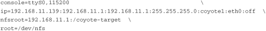
Of course, this would all be on one line. The ip= parameter is defined in .../Documentation/filesystems/nfsroot.txt and has the following syntax, all on one line:
![]()
Here, client-ip is the target’s IP address; server-ip is the address of the NFS server; gw-ip is the gateway (router), in case the server is on a different subnet; and netmask defines the class of IP addressing. hostname is a string that is passed as the target hostname; device is the Linux device name, such as eth0; and autoconf defines the protocol used to obtain initial IP parameters, such as BOOTP or DHCP. It can also be set to off for no autoconfiguration.
9.9 Pseudo File Systems
A number of file systems fall under the category of Pseudo File Systems in the kernel-configuration menu. Together they provide a range of facilities useful in a wide range of applications. For additional information, especially on the /proc file system, spend an afternoon poking around this useful system facility. References to additional reading material can be found in the last section of this chapter.
9.9.1 /proc File System
The /proc file system takes its name from its original purpose: an interface that allows the kernel to communicate information about each running process on a Linux system. Over the course of time, it has grown and matured to provide much more than process information. We introduce the highlights here; a complete tour of the /proc file system is left as an exercise for you.
The /proc file system has become a virtual necessity for all but the simplest of Linux systems, even embedded ones. Many user-level functions rely on the contents of the /proc file system to do their job. For example, the mount command, issued without any parameters, lists all the currently active mount points on a running system, from the information delivered by /proc/mounts. If the /proc file system is unavailable, the mount command silently returns. Listing 9-14 illustrates this on the ADI Engineering Coyote board.
Listing 9-14. Mount Dependency on /proc
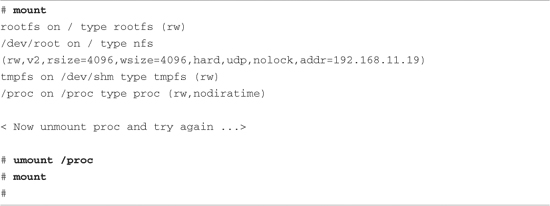
Notice in Listing 9-14 that /proc itself is listed as a mounted file system, as type proc mounted on /proc. This is not doublespeak; your system must have a mount point called /proc at the top-level directory tree as a destination for the /proc file system to be mounted on.7. To mount the /proc file system, use the mount command, as with any other file system:
$ mount -t proc /proc /proc
The general form of the mount command, from the man page, is:
mount [-t fstype] something somewhere
In the preceding invocation, we could have substituted none for /proc, as follows:
$ mount -t proc none /proc
This looks somewhat less like doublespeak. The something parameter is not strictly necessary, because /proc is a pseudo file system, not a real physical device. However, specifying /proc as in the earlier example helps remind us that we are mounting the /proc file system on the /proc directory (or, more appropriately, on the /proc mount point).
Of course, by this time, it might be obvious that to get /proc file system functionality, it must be enabled in the kernel configuration. This kernel-configuration option can be found on the File Systems submenu under the category Pseudo File Systems.
Each user process running in the kernel is represented by an entry in the /proc file system. For example, the init process introduced in Chapter 6 is always assigned the process ID (PID) of 1. Processes in the /proc file system are represented by a directory that is given the PID number as its name. For example, the init process with a PID of 1 would be represented by a /proc/1 directory. Listing 9-15 shows the contents of this directory on our embedded Coyote board.
Listing 9-15. init Process /proc Entries
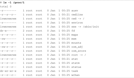
These entries, which are present in the /proc file system for each running process, contain much useful information, especially for analyzing and debugging a process. For example, the cmdline entry contains the complete command line used to invoke the process, including any arguments. The cwd and root directories contain the processes’ view of the current working directory and current root directory.
One of the more useful entries for system debugging is the maps entry. This contains a list of each virtual memory segment assigned to the program, along with attributes for each. Listing 9-16 is the output from /proc/1/maps in our example of the init process.
Listing 9-16. init Process Memory Segments from /proc

The usefulness of this information is readily apparent. You can see the program segments of the init process itself in the first two entries. You can also see the memory segments used by the shared library objects being used by the init process. The format is as follows:
vmstart-vmend attr pgoffset devname inode filename
Here, vmstart and vmend are the starting and ending virtual memory addresses, respectively. attr indicates memory region attributes, such as read, write, and execute, and tells whether this region is shareable. pgoffset is the page offset of the region (a kernel virtual memory parameter). devname, displayed as xx:xx, is a kernel representation of the device ID associated with this memory region. The memory regions that are not associated with a file are also not associated with a device—thus the 00:00. The final two entries are the inode and file associated with the given memory region. Of course, if a memory segment is not accociated with a file, the inode field will contain 0. These are usually data segments.
Other useful entries are listed for each process. The status entry contains information about the running process, including items such as the parent PID, user and group IDs, virtual memory usage, signals, and capabilities. More details can be obtained from the references at the end of this chapter.
Some frequently used /proc entries are cpuinfo, meminfo, and version. The cpuinfo entry lists attributes that the kernel discovers about the processor(s) running on the system. The meminfo entry provides statistics on the total system memory. The version entry mirrors the Linux kernel version string, together with information on what compiler and machine were used to build the kernel.
The kernel generates many more useful /proc entries; we have only scratched the surface of this useful subsystem. Many utilities have been designed for extracting and reporting information contained in the /proc file system. Two popular examples are top and ps, which every embedded Linux developer should be intimately familiar with. These are introduced in Chapter 13. Other utilities useful for interfacing with the /proc file system include free, pkill, pmap, and uptime. See the procps package for more details.
9.9.2 sysfs
Like the /proc file system, sysfs is not representative of an actual physical device. Instead, sysfs models specific kernel objects such as physical devices and provides a way to associate devices with device drivers. Some agents in a typical Linux distribution depend on the information on sysfs.
We can get some idea of what kinds of objects are exported by looking directly at the directory structure exported by sysfs. Listing 9-17 shows the top-level /sys directory on our Coyote board.
Listing 9-17. Top-Level /sys Directory Contents
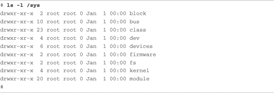
sysfs provides a top-level subdirectory for several system elements, including the system buses. For example, under the block subdirectory, each block device is represented by a subdirectory entry. The same holds true for the other directories at the top level.
Most of the information stored by sysfs is in a format more suitable for machines rather than humans to read. For example, to discover the devices on the PCI bus, you could look directly at the /sys/bus/pci subdirectory. On our Coyote board, which has a single PCI device attached (an Ethernet card), the directory looks like this:
![]()
Parts of the output were trimmed for clarity. This entry is actually a symbolic link pointing to another node in the sysfs directory tree. The name of the symbolic link is the kernel’s representation of the PCI bus, and it points to a devices subdirectory called pci0000:00 (the PCI bus representation). This subdirectory contains a number of subdirectories and files representing attributes of this specific PCI device. As you can see, the data is rather difficult to discover and parse.
A useful utility can help you browse the sysfs file system directory structure. Called systool, it comes from the sysfsutils package found on sourceforge.net. Here is how systool would display the PCI bus from the previous discussion:
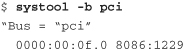
Again we see the kernel’s representation of the bus and device (0f), but this tool displays the vendor ID (8086 = Intel) and device ID (1229 = eepro100 Ethernet card) obtained from the /sys/devices/pci0000:00 branch of /sys, where these attributes are kept. Executed with no parameters, systool displays the top-level system hierarchy. Listing 9-18 is an example from our Coyote board.
Listing 9-18. Output from systool
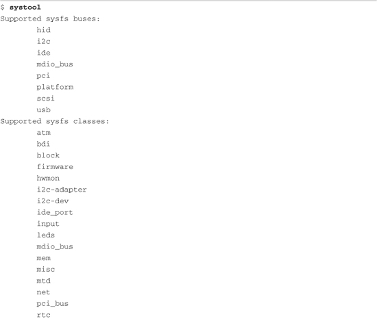
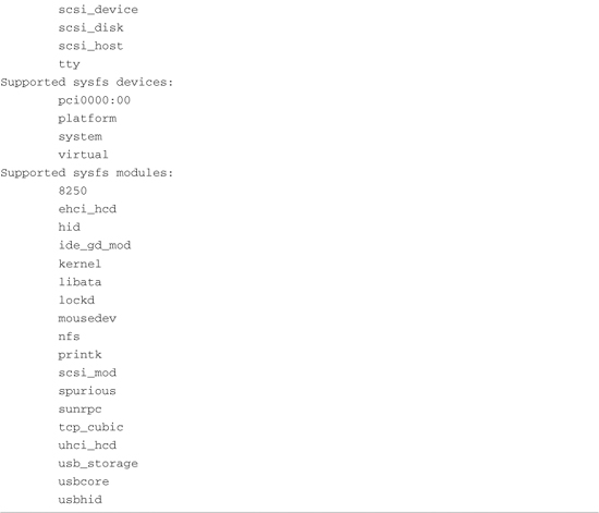
You can see from this listing the variety of system information available from sysfs. Many utilities use this information to determine the characteristics of system devices or to enforce system policies, such as power management and hot-plug capability.
You can learn more about sysfs from http://en.wikipedia.org/wiki/Sysfs and the references found there.
9.10 Other File Systems
Linux supports numerous file systems. Space does not permit us to cover all of them. However, you should be aware of some important file systems frequently found in embedded systems.
The ramfs file system is best considered from the context of the Linux source code module that implements it. Listing 9-19 reproduces the first several lines of that file.
Listing 9-19. Linux ramfs Source Module Comments
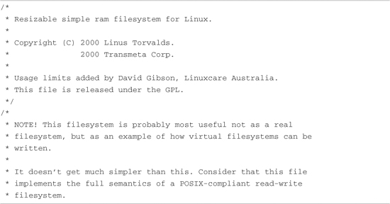
This module was written primarily as an example of how virtual file systems can be written. One of the primary differences between this file system and the ramdisk facility found in modern Linux kernels is its capability to shrink and grow according to its use. A ramdisk does not have this property. This source module is compact and well written. It is presented here for its educational value. You are encouraged to study this example if you want to learn more about Linux file systems.
The tmpfs file system is similar to and related to ramfs. Like ramfs, everything in tmpfs is stored in kernel virtual memory, and the contents of tmpfs are lost on power-down or reboot. The tmpfs file system is useful for fast temporary file storage. A good example of tmpfs use is to mount your /tmp directory on a tmpfs. It improves performance for applications that use many small temporary files. This is also a great way to keep your /tmp directory clean, because its contents are lost on every reboot. Mounting tmpfs is similar to any other virtual file system:
# mount -t tmpfs /tmpfs /tmp
As with other virtual file systems such as /proc, the first tmpfs parameter in this mount command is a “no-op.” In other words, it could be the word none and still function. However, it is a good reminder that you are mounting a virtual file system called tmpfs.
9.11 Building a Simple File System
It is straightforward to build a simple file system image. Here we demonstrate the use of the Linux kernel’s loopback device. The loopback device enables the use of a regular file as a block device. In short, we build a file system image in a regular file and use the Linux loopback device to mount that file in the same way any other block device is mounted.
To build a simple root file system, start with a fixed-sized file containing all 0s:
# dd if=/dev/zero of=./my-new-fs-image bs=1k count=512
This command creates a file of 512KB containing nothing but 0s. We fill the file with 0s to aid in compression later and to have a consistent data pattern for uninitialized data blocks within the file system. Exercise caution when using the dd command. Executing dd with no boundary (count=) or with an improper boundary can fill up your hard drive and possibly crash your system. dd is a powerful tool; use it with the respect it deserves. Simple typos in commands such as dd, executed as root, have destroyed countless file systems.
When we have the new image file, we actually format the file to contain the data structures defined by a given file system. In this example, we build an ext2 file system. Listing 9-20 details the procedure.
Listing 9-20. Creating an ext2 File System Image
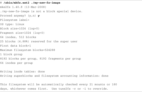
Like dd, the mkfs.ext2 command can destroy your system, so use it with care. In this example, we asked mkfs.ext2 to format a file rather than a hard drive partition (block device) for which it was intended. As such, mkfs.ext2 detected that fact and asked us to confirm the operation. After confirming, mkfs.ext2 proceeded to write an ext2 superblock and file system data structures into the file. We can then mount this file like any block device, using the Linux loopback device:
# mount -o loop ./my-new-fs-image /mnt/flash
This command mounts the file my-new-fs-image as a file system on the mount point named /mnt/flash. The mount point name is unimportant; you can mount it wherever you want, as long as the mount point exists. Use mkdir to create your mount point.
After the newly created image file is mounted as a file system, we are free to make changes to it. We can add and delete directories, make device nodes, and so on. We can use tar to copy files into or out of it. When the changes are complete, they are saved in the file, assuming that you didn’t exceed the size of the device. Remember, using this method, the size is fixed at creation time and cannot be changed.
9.12 Summary
This chapter introduced a variety of file systems in use on both desktop/server Linux systems and embedded systems. File systems specific to embedded use and especially Flash file systems were described. The important pseudo file systems also were covered.
• Partitions are the logical division of a physical device. Numerous partition types are supported under Linux.
• A file system is mounted on a mount point in Linux. The root file system is mounted at the root of the file system hierarchy and is referred to as /.
• The popular ext2 file system is mature and fast. It is often found on embedded and other Linux systems such as Red Hat and the Fedora Core series.
• The ext3 file system adds journaling on top of the ext2 file system for better data integrity and system reliability.
• ReiserFS is another popular and high-performance journaling file system found on many embedded and other Linux systems.
• JFFS2 is a journaling file system optimized for use with Flash memory. It contains Flash-friendly features such as wear leveling for longer Flash memory lifetime.
• cramfs is a read-only file system perfect for small-system boot ROMs and other read-only programs and data.
• NFS is one of the most powerful development tools for the embedded developer. It can bring the power of a workstation to your target device. Learn how to use NFS as your embedded target’s root file system. The convenience and time savings will be worth the effort.
• Many pseudo file systems are available on Linux. A few of the more important ones were presented here, including the /proc file system and sysfs.
• The RAM-based tmpfs file system has many uses for embedded systems. Its most significant improvement over traditional ramdisks is the capability to resize itself dynamically to meet operational requirements.
9.12.1 Suggestions for Additional Reading
“Design and Implementation of the Second Extended Filesystem”
Rémy Card, Theodore Ts’o, and Stephen Tweedie
First published in the Proceedings of the First Dutch International Symposium on Linux
http://e2fsprogs.sourceforge.net/ext2intro.html
“A Non-Technical Look Inside the EXT2 File System”
Randy Appleton
www.linuxjournal.com/article/2151
Red Hat’s New Journaling File System: ext3
Michael K. Johnson
www.redhat.com/support/wpapers/redhat/ext3/
Reiser4 File System
http://en.wikipedia.org/wiki/Reiser4
JFFS: The Journaling Flash File System
David Woodhouse
http://sources.redhat.com/jffs2/jffs2.pdf
README file from the cramfs project
Unsigned (assumed to be the project author)
http://sourceforge.net/projects/cramfs/
NFS home page
http://nfs.sourceforge.net
The /proc file system documentation
www.tldp.org/LDP/lkmpg/2.6/html/c712.htm
“File System Performance: The Solaris OS, UFS, Linux ext3, and ReiserFS”
A technical whitepaper
Dominic Kay
www.sun.com/software/whitepapers/solaris10/fs_performance.pdf