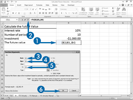
If you have $1,000 and you plan to invest it at 10 percent interest, compounded annually for ten years, the amount you will receive at the end of ten years is called the future value (FV) of $1,000. You can use Excel's FV function to calculate the amount you will receive.
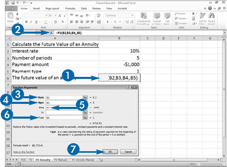
An annuity is a series of payments where each payment is the same amount, the period between payments is the same, the interest rate for each period is constant, and the interest is compounded. If you deposit $1,000 per year for five years and receive 10 percent interest, compounded annually, the amount you receive at the end of five years is the future value of an annuity. You can also use Excel's FV function to compute the future value of an annuity.
When you are working with the FV function, negative numbers are cash outflows and positive numbers are cash inflows. Enter a negative number when you are making a payment. Enter a positive number when you are receiving cash. Although the transaction is called a payment, note that there are two sides to the transaction. For example, when you make a payment to the bank, the bank considers the transaction a cash receipt.
Excel's FV function asks for five pieces of information: Rate, the interest rate; Nper, the number of payment periods, Pmt, the amount of each payment; PV, your investment — the value for which you are trying to find the future value; and Type, a number indicating when payments are due. If you make your payments at the beginning of the period, enter a 1 as the Type. If you make your payments at the end of the period, leave Type blank or enter 0.
Calculate Future Value
Calculate a Future Value


The Function Arguments dialog box appears.

Note: If you make payments more than once annually, divide the interest rate by the number of payments per year.

Note: If you make payments more than once annually, multiply the number of years by the number of payments per year.


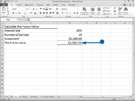
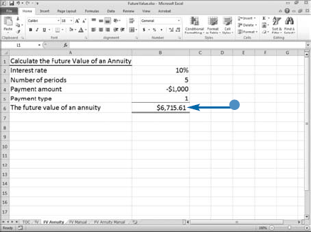
Excel calculates the future value.
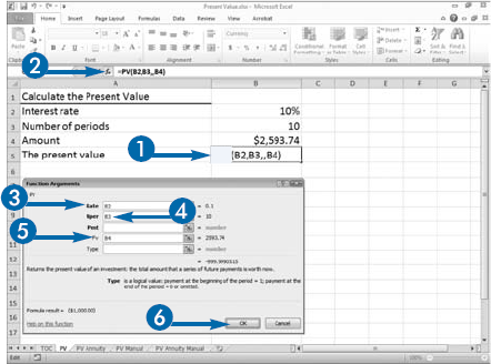
Investors use the concept of present value (PV) to recognize the time value of money. Because an investor can receive interest, $1,000 today is worth less than $1,000 ten years from today. For example, if an investor invests $1,000 today at 10 percent interest per year, compounded annually, in ten years the investor will have $2,593.74. Therefore, the present value of $2,593.74 at 10 percent, compounded annually, for 10 years is $1,000. Or, worded differently, $1,000 today is worth $2,593.74 ten years from today.
You can use the following formula to calculate the present value of an investment: pv = a/((1+i)^n) where pv equals the present value, a equals the amount you want to find the present value of, i equals the annual interest rate, and n equals the number of periods. To find the present value of the $2,593.74, enter =2593.74/((1+.10)^10) or use Excel's PV function.
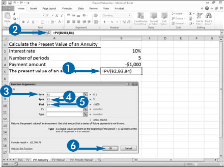
An annuity is a series of payments where each payment is the same amount, the period between payments is the same, the interest rate for each period is constant, and the interest is compounded. For example, a payment of $1,000 per year for five years at 10 percent interest compounded at the end of each year is an annuity. To find the present value of an annuity, you can add the present values of each payment or you can use Excel's PV function. Excel's PV function needs five pieces of information: Rate, the interest rate; Nper, the number of payment periods; Pmt, the amount of each payment; PV, the value you are trying to find the present value of; and Type, a number indicating when payments are due.
Calculate Present Value
Calculate the Present Value
The Function Arguments dialog box appears.
Note: If you make payments more than once annually, divide the interest rate by the number of payments per year.
Note: If you make payments more than once annually, multiply the number of years by the number of payments per year.
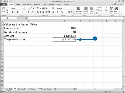
Excel calculates the present value.
Calculate the Present Value of an Annuity
The Function Arguments dialog box appears.
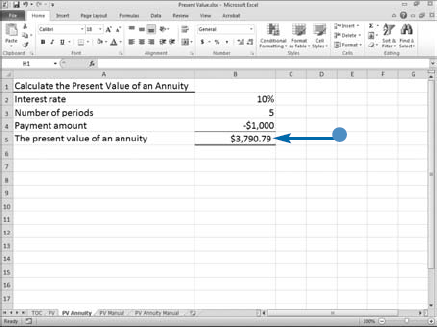
Excel calculates the present value of an annuity.
You can use Excel's PMT function (PMT is short for payment) when buying a house or car. This function enables you to compare loan terms and make an objective decision based on factors such as the interest rate and the amount of the monthly payment.
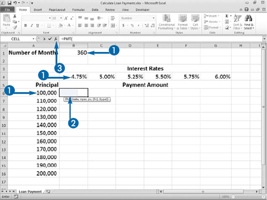
You can calculate loan payments in many ways when using Excel, but the PMT function may be the simplest method because you simply enter information into the Function Wizard. You can create a loan calculator that shows how varying the elements affect the results. Place the labels Principal, Interest Rates, and Number of Months in your worksheet. Then type their respective values. For example, you can calculate the payment amount at 4.75 percent, 5 percent, and 5.25 percent to see the effect of changing the annual interest.
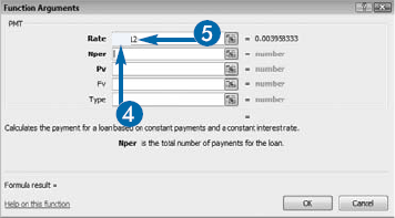
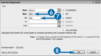
The PMT function requires three pieces of information. To calculate the periodic rate, you enter an annual interest rate such as 5 percent (.05) and then divide the interest rate by the number of payments you make per year. For example, if you pay monthly, enter .05/12 as the Rate. Enter the number of loan periods for the loan you are seeking for the Nper. For example, if your loan is for 30"years and you will make payments monthly, multiply 30 years by 12 months to get 360 periods and then type"360 in the Nper field. For Pv, enter the amount of the loan. The PMT function calculates the amount of each payment. The payment amount appears surrounded by parentheses, signifying that the number is negative, and a cash outflow.
Calculate Loan Payments
The Function Arguments dialog box appears.
Make the row reference absolute.
Note: See Chapter 4 to learn more about absolute and relative cell references.
Make both the column and row reference absolute.

Make the column reference absolute.

The result appears in the cell.
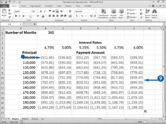
Note: The result shows the amount of a single loan payment.

Note: See Chapter 3 to learn how to copy and paste.
Excel calculates the loan payments.
When you use the PMT function to calculate a monthly loan payment, Excel calculates the total of the principal and the interest. See the previous section, "Calculate Loan Payments," to learn more about using the PMT function. If you need to know the principal or the interest portion of a payment, you can use the PPMT function or the IPMT function.
An annuity is a series of payments where each payment is the same amount, the period between payments is the same, the interest rate for each period is constant, and the interest is compounded. The PPMT function finds the principal portion of a loan payment when the loan is an annuity. The amount of the principal portion of a loan changes after each payment. The PPMT function needs six pieces of information: Rate, the interest rate; Per, the number of the payment for which you want to obtain the principal; Nper, the total number of payments; Pv, the loan amount; Fv, the future value amount; and Type, a number that indicates if payments are due at the end of the period or the beginning of the period.
The IPMT function finds the interest portion of a loan payment when the loan is an annuity. The amount of the interest portion of a loan changes after each payment. The IPMT function also needs six piece of information: Rate, the interest rate; Per, the number of the loan payment for which you want to obtain the principal; Nper, the total number of payments; Pv, the loan amount; Fv, the future value amount; and Type, a number that indicates if payments are due at the end of the period or the beginning of the period. For each period, the principal plus the interest should equal the payment amount.
Calculate Principal or Interest
Calculate the Principal
The Function Arguments dialog box appears.
Note: If you make payments more than once annually, divide the interest rate by the number of payments per year.
Note: If you make payments more than once annually, multiply the number of years by the number of payments per year.
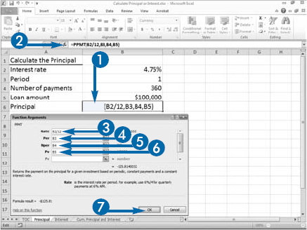
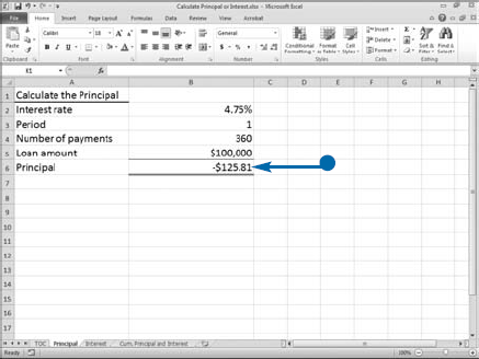
Excel calculates the principal.
The Function Arguments dialog box appears.
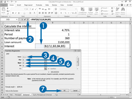
Excel calculates the interest.

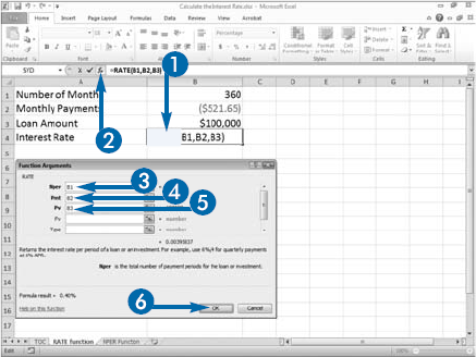
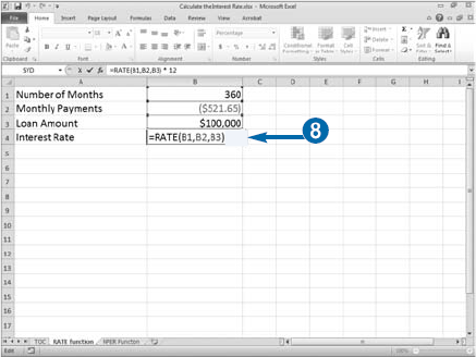
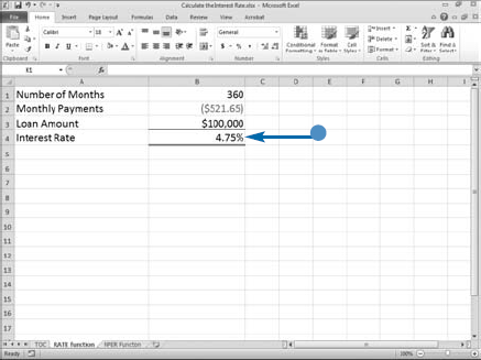
You can use Excel's RATE function to calculate the interest rate associated with an annuity. An annuity is a series of payments where each payment is the same amount, the period between payments is the same, the interest rate for each time period is constant, and the interest is compounded. Generally speaking, a bank loan is an annuity. If you receive a bank loan for $100,000 and you pay $521.65 monthly for 360 months, you can use the RATE function to calculate the interest rate.
When you are working with the RATE function, negative numbers are cash outflows and positive numbers are cash inflows. Your monthly payment of $521.65 is a cash outflow, so you enter it as a negative number. Your loan of $100,000 is a cash inflow, so you enter it as a positive number.
Excel's RATE function asks for six pieces of information: Nper, the number of payment periods; Pmt, the amount of each payment; Pv, the amount of the loan; Fv, the future value you want to attain; and Type, a number indicating when payments are due. If you make your payments at the beginning of the period, enter 1 as the Type argument.
Optionally, you can provide an additional argument, your best-guess estimate as to the rate of return. Calculating the rate is an iterative process where Excel starts with an initial guess for the rate and attempts to refine that guess to obtain the answer. The default value, if you do not provide an estimate is .10, representing a 10 percent rate of return. If after 20 tries Excel cannot return a value, it returns a #NUM! error. You should enter a value in the Guess field and try again.

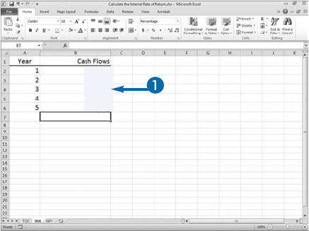
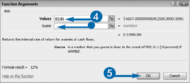
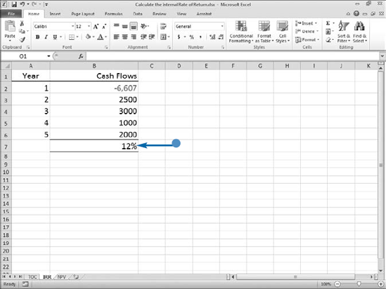
You can use Excel's Internal Rate of Return (IRR function) to calculate the internal rate of return on an investment. When you are using the IRR function, the cash flows do not have to be equal, but they must occur at regular intervals. As an example, you make a loan of $6,607 on January 1, year 1. You receive payments every January 1 for four succeeding years. You can use the IRR function to determine the interest rate you receive on the loan.
Your loan of $6,607 is a cash outflow, so you enter it as a negative number. Each payment is a cash inflow, so you enter them as positive numbers. When using the IRR function, you must enter at least one positive and one negative number.
Optionally, you can provide an additional piece of information, your best-guess estimate as to the rate of return. Calculating the rate is an iterative process where Excel starts with an initial guess for the rate and attempts to refine that guess to obtain the answer. The default value, if you do not provide an estimate, is .10, representing a 10 percent rate of return. Your estimate gives Excel a starting point at which to calculate the RATE. If after 20 tries Excel cannot return a value, it returns a #NUM! error. You should enter a value in the Guess field and try again.
Excel's IRR function has strict assumptions. Cash flows must be regularly timed and take place at the same point within each payment period. IRR may perform less reliably for inconsistently timed payments and variable interest rates. Excel uses the order of the values to interpret the cash flows, so enter your values in the proper sequence.

Buildings, cars, trucks, and equipment are all examples of depreciable assets. Accountants consider an asset depreciable if it has a useful life of more than one year but does not last indefinitely. Because accountants want to match the cost of an asset with the revenue produced from using the asset, they allocate the cost of a depreciable asset over the life of the asset. Accountants use several depreciation methods to allocate cost.
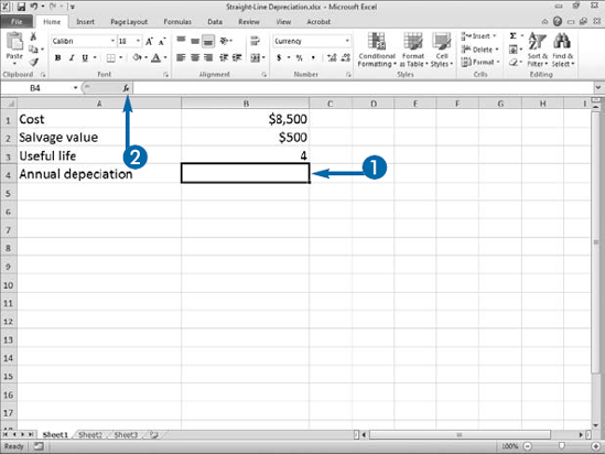
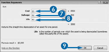
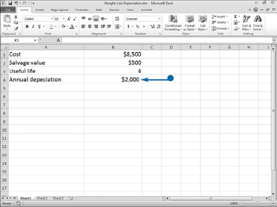
The straight-line method of depreciation allocates depreciation evenly over the useful life of the asset. Salvage value is the value of an asset once its useful life has expired. To calculate straight-line depreciation, you take the cost of the asset, subtract any salvage value, and then divide by the useful life of the asset. The result is the amount of depreciation allocated to each period. For example, you purchase a piece of equipment on January 1 for $8,500, the equipment has a useful life of four years, and it can be sold for $500 at the end of four years. To calculate the annual depreciation, you use the formula = (8500–500)/4. The result, 2,000, is the annual depreciation.
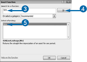
You can use Excel's SLN function to calculate straight-line depreciation. The SLN function asks for three pieces of information: Cost, the initial cost of the asset; Salvage, the salvage value of the asset; and Life, the life of the asset in periods. If you purchase an asset mid-year, you may want to calculate depreciation in months. When calculating depreciation in months, enter the number of months that make up the useful life of the asset as the Life.
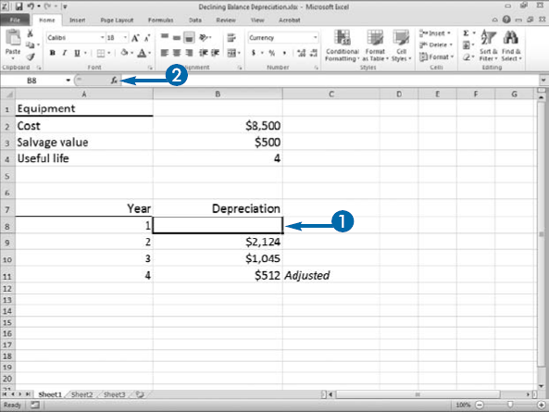
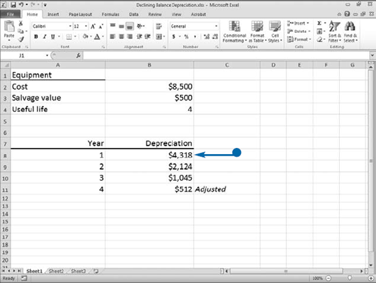
When calculating depreciation, accountants try to match the cost of an asset with the revenue it produces. Some assets produce more in earlier years than they do in later years. For those assets, accountants use accelerated methods of depreciation. Accelerated methods of depreciation take more depreciation in the earlier years than they do in the later years. Declining balance is an accelerated method of depreciation. You can use Excel's DB function to calculate declining balance depreciation.
The carrying value is the cost of an asset minus the total depreciation taken to date. When you use the declining balance depreciation method, you calculate a rate. The rate could be 50 percent, for example. You apply the rate to the carrying value to get the annual depreciation. Because the carrying value goes down each year, your depreciation is higher in earlier years than it is in later years. Excel uses the following formula to calculate the rate: rate = 1–((salvage/cost)^(1/life)), rounded to three decimal places. After Excel calculates the rate, it uses the following formula to calculate depreciation: depreciation =(cost-depreciation from prior periods)* rate. The first and last periods are special. The formula for the first period is cost*rate month/12. The formula for the last period is ((cost–total depreciation for prior periods)*rate*12-month))/12.
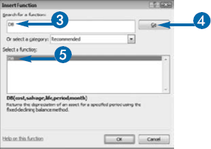
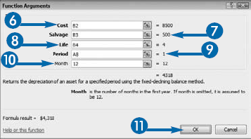
The DB function asks for five pieces of information: Cost, the cost of the asset; Salvage, the salvage value; Life, the useful life; Period, the period for which you are calculating depreciation; and Month, the number of months in the first year. If you leave the Month argument blank, Excel assumes the number of months in the first year to be 12.
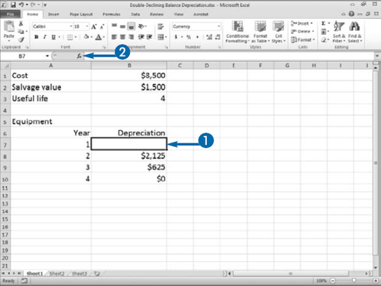
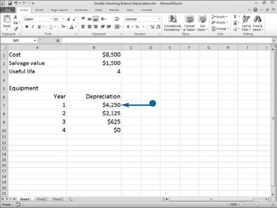
Like the declining balance method discussed in the previous section, double-declining balance is an accelerated depreciation method. The carrying value is the cost of an asset minus the amount of depreciation taken to date. Salvage value is the amount you can sell an asset for after its useful life. Double-declining balance takes the rate you would apply by using straight-line depreciation, doubles it, and then applies the doubled rate to the carrying value of the asset. For example, under the straight-line method of depreciation, if you purchase an asset that has a useful life of four years, you would take depreciation at a rate of 1/4th per year or 25 percent. Under the double-declining balance method, you double the 25 percent and take 50 percent of the carrying value as the annual depreciation; however, you do not depreciate the asset below the salvage value. You can use the DDB function to calculate double-declining balance depreciation. The DDB function uses the following formula to calculate double-declining balance depreciation:
=MIN((cost-depreciation taken to date)*
(rate),(cost-salvage value-depreciation taken to date))
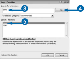
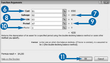
You must supply the DDB function with the following information: Cost, the cost of the asset; Salvage, the amount you can sell the asset for after its useful life; Life, the useful life in periods; Period, the period for which you are calculating depreciation; and Factor, the rate at which the balance declines. If you are doubling the straight-line rate, enter 2 as the Factor or leave the Factor argument blank. If you want to use a rate other than twice the straight-line rate, enter the factor you want to use. For example, enter 1.5 if you want to use a rate of 150 percent.
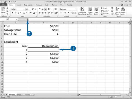
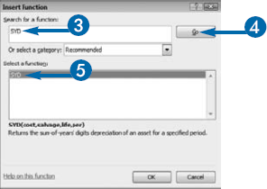
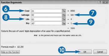
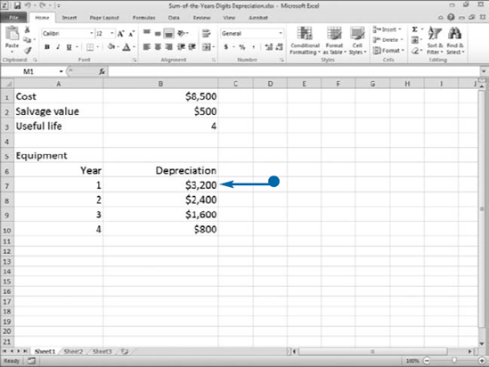
When calculating depreciation, accountants try to match the cost of an asset with the revenue it produces. Some assets produce more in earlier years than they do in later years. For those assets, accountants use accelerated methods of depreciation. Sum-of-the-years-digits is an accelerated depreciation method. When you calculate sum-of-the-years-digits depreciation manually, you use a fraction to calculate annual depreciation. The numerator of the fraction is the remaining years of useful life. The denominator is the sum of the digits that make up the useful life. For example, if you want to calculate depreciation for the first year of an asset with a useful life of four years, cost of 8,500, and a salvage value of 500, the numerator is 4 and the denominator is 10, the sum of 1+2+3+4. You multiply the fraction by the cost of"the asset minus the salvage value. The calculation for"the first year is 4/10*(8500–500), or 3,200; the calculation for the second year is 3/10*(8500–500), or 2,400; the calculation for the third year is 2/10*(8500–500), or 1,600; and the calculation for the fourth year is 1/10*(8500–500), or 800. You can use the SYD function to calculate sum-of-the-years-digits depreciation in Excel. The SYD function uses the following formula:
SYD=((cost–salvage)*(life–per+1)*2)/
 ((life)*(life+1))
You must supply the SYD function with the following information: Cost, the cost of the asset; Salvage, the amount you can sell the asset for after its useful life; Life, the useful life in periods; and Per, the period for which you are calculating depreciation.