
9.3 Several Categorical Factors: the Full Factorial Design
We frequently expect the response in an experiment to be affected by several factors. If so, it is interesting to find out which factor has the strongest effect on the response. Another important question is if the effects are separate or if the way in which the factors are combined is important. These questions can be answered by full factorial experiments.
We will begin by a case with only two factors, since this is convenient for understanding. The design is shown in Table 9.1, where the columns represent the two factors and the rows correspond to the investigated factor combinations, or treatments. We may note that all the possible combinations are present. To understand how the effects of the factors still can be separated, we will introduce the concept of orthogonality. This requires a brief mathematical digression, but we will soon be back on track again.
Table 9.1 Two-level full factorial design with two factors.
| A | B |
| −1 | −1 |
| 1 | −1 |
| −1 | 1 |
| 1 | 1 |
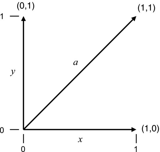
Mathematicians discern between two types of quantities: scalars and vectors. Numbers in general only have size and are called scalars. Scalars are used to describe things like the outside temperature or the atmospheric pressure. Vectors have both size and direction and are expressed in terms of coordinates. The wind velocity is one example. The plane in Figure 9.2 is defined by two vectors, x and y, each with a length of one unit. They represent the two principal directions in which it is possible to move in that plane. Any vector in the plane can be expressed in terms of (x,y) coordinates. The coordinates of the x-vector are (1,0), the y-vector is expressed as (0,1) and the vector a has the coordinates (1,1). All these coordinates can be seen as instructions for getting from the origin to a certain point in the x–y plane: x says “move one unit in the x-direction”, y says “move one unit in the y-direction” and a says “move one unit along x and then one along y”. The last instruction is just the combination of the first two and, for this reason, a is said to be a linear combination of x and y. Specifically, we may obtain a by adding the x- and y-coordinates of x and y separately, since (1 + 0, 0 + 1) gives us (1,1). As x and y are at right angles to each other they are, by definition, orthogonal. Since a can be obtained by combining the other two, it is not orthogonal to any of them. In mathematical terms, a set of orthogonal vectors is characterized by the fact that none can be obtained by a linear combination of the others.
Figure 9.2 Plane defined by two vectors, x and y. The third vector a is a linear combination of the two.
If two vectors are orthogonal the inner product between them is zero. We obtain the inner product by multiplying the respective elements of the two vectors and summing up the products. For the orthogonal x- and y-vectors this gives (1 × 0) + (0 × 1) = 0. If we apply this calculation to the two columns of Table 9.1 we see that they too are orthogonal to each other:
(9.1) ![]()
Now, what on earth does this have to do with experimental design? Well, in a multifactor experiment we want to separate the effects of the factors on a response variable and we may do this by utilizing an orthogonal test matrix. As we have seen, the design in Table 9.1 is one such example, since the combination of settings in each column is orthogonal to the other. The easiest way to understand how this works and why it is useful is to show a simple example.
Imagine that you are interested in three categorical factors, A, B and C. They could, for instance, be factors of interest for the amount of wear on a bearing surface. A could be a manipulation of the surface of the shaft, B a manipulation of the bearing, and C an additive in the lubricant. Let us say that you want to investigate the amount of wear that you get with and without these factors. This means that each factor will have two settings in the test matrix: “with” and “without”. We will simply call these settings +1 and −1. Table 9.2 shows the test matrix for all possible combinations; the levels are denoted by “+” and “−” signs for simplicity. The design is also shown graphically as a cube.
Table 9.2 Two-level full factorial design with three factors.

The vertical columns correspond to different factors and the horizontal rows to different treatments. In this case the treatments are combined so as to obtain orthogonal columns. We may confirm this by verifying that the inner products between the columns are zero.
The orthogonal test matrix is obtained by filling out the first column with alternate “+” and “–” signs. The second column is obtained in a similar way but here the signs are repeated in groups of two. In the third column the signs appear in groups of four. We may expand this test matrix to any number, n, of factors, with the groups of signs doubling in size for each consecutive column. The three factors in Table 9.2 thereby give us 23 = 8 rows and, for this reason, this is sometimes called a 23 design. The ordering of the treatments is called Yates order and the resulting test matrix is called a full factorial design.
In addition to providing an orthogonal test matrix the full factorial design tests all possible combinations of factor levels. As the design in Table 9.2 tests each factor at a high and low setting it is called a two-level full factorial design. The design can be extended to more levels. For a three-level design we usually denote the levels by “−”, “0” and “+” signs. With three factors the number of rows in the matrix becomes 33 = 27. In general, the number of treatments, k, in a full factorial design is given by:
where l is the number of levels and n is the number of factors. Figure 9.3 shows a graphical comparison of a two-level and a three-level full factorial design with three factors.
Figure 9.3 Comparison of a two-level and a three-level full factorial experiment.
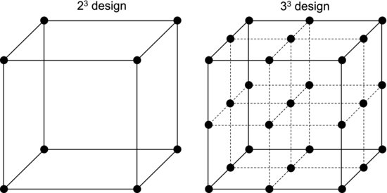
Table 9.3 The full factorial design in Table 9.2 supplemented with columns for interactions.
Let us look at some data to see why the orthogonality is convenient when analyzing a full factorial experiment. In Table 9.3 we have taken the test matrix in Table 9.2 and added factor interactions by multiplying the three columns A, B and C with each other. The resulting matrix contains columns corresponding to the three factors, three two-way interactions and one three-way interaction. Note that these interactions do not have to be considered during the experiment; they are calculated afterwards. The column at the far right is a measured response that results from the settings of A, B and C. It could, for instance, be the outcome of an abrasive wear test. If you wonder about the numbers below the table their meaning will soon become clearer.
Now, if we take the inner product between a factor column and the response column we get a measure of the linear association between them. If there is no relationship between the factor and the response they are linearly independent. In other words, they are orthogonal to each other and the inner product will be zero. Similarly, a large inner product translates into a strong association between the factor and the response. This is because taking the inner product between two vectors is very similar to calculating their correlation coefficient, as described in Equation 8.8. Since the factor columns are linearly independent of each other this amounts to a method for complete separation of each factor's effect on the response. It goes without saying that this is very useful to an experimenter: we design an experiment where we vary all factors simultaneously but, still, their effects on the response can be completely isolated.
Recall that if the test plan were not orthogonal, one column could be obtained from a linear combination of the others. This means that the factors’ effects on the response would be mixed with each other. This is why it is difficult to see clear relationships in observational studies where the data never originate from orthogonal test plans. In observational data, a multitude of factors vary haphazardly and simultaneously and this causes their effects to bleed into each other. This problem is called collinearity, a word describing that the factor columns are not linearly independent.
Continuing with the numbers below Table 9.3, we will first calculate what is called the effects of the factors. The effect measures the magnitude of the response that results from a change in a factor. Looking at the first column we see that there are four measurements at the low setting of A (−1) and four at the high setting (+1). One way to determine the effect of factor A is to take the difference between the average responses at the high and low settings. In other words, it is the difference between the average responses on the two shaded surfaces of the cube in Table 9.2. This difference will say something about whether the response tends to increase or decrease when A increases from −1 to +1 and, if so, how much. The effect of A is explicitly calculated as:
(9.3) ![]()
We recognize the denominator as the divisor in Table 9.3, as well as the effect value given there. Factor A, the surface manipulation, seems to be effective since the amount of wear decreases when it is applied. Rearranging the terms we see that this calculation is exactly equivalent to taking the inner product between the A and response columns and dividing by four. The reason that the divisor in Table 9.3 is four is simply that this is the number of measurements at each factor level. In summary, the effect of A measures the average change in the response when A changes from the low level to the high level. Since this calculation only detects the response to a single factor it is called a main effect.
The two-way interactions show if the response to a change in one variable is affected by the setting of another. Let us look at the BC interaction in Table 9.3. With the data in this column we can first calculate the effect of B when C is at the high level; that is, using the four responses that were measured when C was set to +1. Similarly, we can calculate the effect of B when C is set to the low level. Now, the difference between these two effects tells us if the setting of C affects the response to a change in B. The interaction is explicitly calculated as:
Expressed in words, this is half the difference between the effect of B when C is at the high level and the effect of B when C is at the low level. Take a minute to think about this. If the interaction effect is zero this means that the response to a change in B is the same regardless of the setting of C – there is no interaction between them. If the interaction effect is positive it means that the response to a change in B is stronger when C is at the high setting. A negative interaction effect means that the response to a change in B is stronger when C is at the low level. In extreme cases, B may even have the opposite effect on the response at the low setting of C. All of these types of interactions frequently occur in real data. Again, rearranging the terms in Equation 9.4 we see that it is exactly equivalent to taking the inner product between the BC and response columns and dividing by four. As a rough rule of thumb, main effects tend to be largest, two-way interactions tend to be smaller, while three-way and higher interactions usually can be ignored. Looking at the effects calculated at the bottom of Table 9.3 this rule is roughly confirmed, although the AB interaction is relatively large. The rule becomes more manifest in a larger experiment.
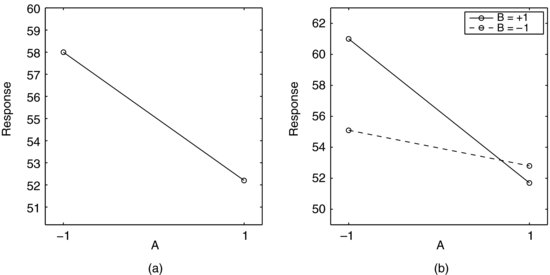
It is always convenient to present results graphically, since it is easier to see relationships in diagrams than in numbers. Data from full factorial experiments are often displayed in effect plots and interaction plots. Figure 9.4a shows an effect plot for factor A in Table 9.3. It simply plots the average responses at the low and high levels of A with a line between the points. Figure 9.4 b is an interaction plot of the AB interaction in Table 9.3 and may require a little more explanation. It could be said to contain two effect plots for factor A. One effect is measured at the high setting of B, the other at the low setting, as indicated in the legend. Since the two lines have different slopes, a single glance shows us that there is an interaction effect and that it is fairly strong. The setting of B clearly affects the response to A.
Figure 9.4 (a) Effect plot of factor A in Table 9.3. (b) Interaction plot of the AB interaction.
We have now learned how to calculate the effects in a full factorial experiment but an important part of the analysis is still missing. After reading the last two chapters we know that measurements always suffer from noise and we need methods to separate the effects from this background variation. Some effects will be strong compared to the noise and some will be weaker, but all effect calculations will return numbers. The problem is to understand which numbers show the random variation and which measure real effects.
We can often find this out graphically by using the now familiar normal plot (Chapter 7). Since the effects are calculated from orthogonal vectors they are independent and can be treated as a random sample. Sorting the effects from the smallest to the largest and plotting them versus their normal scores will produce a normal plot. If there were no effects in the data, the calculated effects would only measure the experimental error. If so, they would be normally distributed and plot on a straight line in the diagram. We hope, of course, that some effects are large compared to the error. If so, they will plot off the line. A relatively large sample is needed to produce a neat normal plot and we will, therefore, move to a two-level four-factor experiment for illustration. The factors A, B, C, and D in Table 9.4 could be any categorical variables suspected of affecting a continuous response variable. They are given in Yates order to make it easier for you to enter them into an Excel spreadsheet. To calculate the interaction effects, the table must be extended to include the six possible two-way interactions (AB, AC, AD, BC, BD, and CD), the four possible three-way interactions (ABC, ABD, ACD, and BCD), and the four-way interaction. In total, this gives us 15 main and interaction effects, which should be sufficient to produce a normal plot.
Table 9.4 Two-level full factorial design with four factors.
Figure 9.5 Normal plot of effects calculated from Table 9.4.
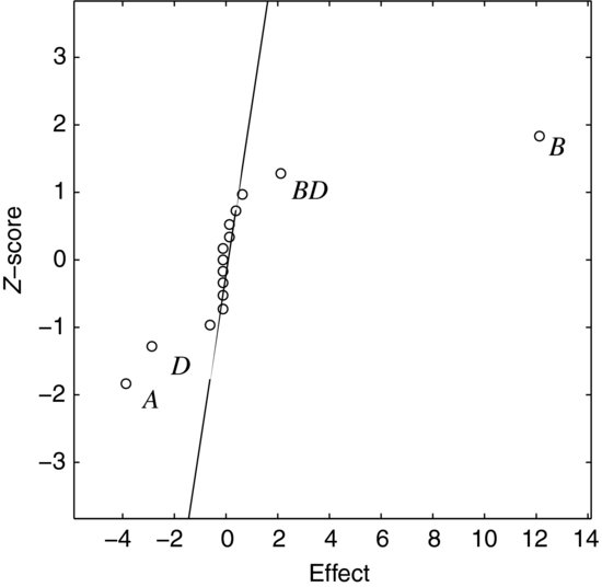
Calculating the effects we see that some are larger than others but we do not easily see which effects stand out from the noise. When plotting them as in Figure 9.5 it only takes a single glance to see that four effects are greater than the noise on the straight line. The largest effect is due to factor B, which plots at the far right of the graph. This means that the response increases when B increases. The second largest effect is due to factor A on the left. This effect is negative, meaning that the response decreases when A increases. To put it simply, factors plotting to the right are positively correlated with the response, while those plotting to the left are negatively correlated. The other two significant terms are D and the BD interaction.
Strictly, it is not correct to talk about correlation when the factors are categorical, so keep in mind that we refer to the coded values −1 and +1, which were arbitrarily assigned to the factor levels. Another way of separating the statistically significant effects from the noise is to apply a t-test to the effects. This method will be introduced later in this chapter, in connection with continuous factors and regression.
Before finishing this section we should discuss some experimental precautions that are commonly used in full factorial experiments. First of all, a full factorial experiment should never be run in Yates order. Factor D in Table 9.4, for example, would then be at the low setting during the entire first half of the experiment and at the high setting during the second half. There could be a background factor that drifts slowly during the measurements, for instance if they are made during a run-in phase. If the response were to increase due to this drift the average response would be lower during the first measurements. This, in turn, means that factor D would show a false effect due to this drift. To safeguard against false background effects, the run order should always be randomized. It is quite easy to produce a column of random numbers alongside the test matrix in Excel, for example using the RAND or RANDBETWEEN functions. The test matrix can then be randomized by sorting all the columns according to these random numbers.
We also need to estimate the experimental error. This is normally not done using the graphical approach in Exercise 9.4 but by using regression analysis. Recall from Chapter 8 that it costs one degree of freedom to estimate a parameter in a regression model and that additional degrees of freedom are needed to estimate the error. This means that the table with factor and interaction columns must be taller than it is wide, since each column is associated with one parameter. Such a table is obtained by replicating the measurements one or several times. To avoid background effects, the replicates should be run in random order and be mixed with the original measurements. You may note that none of the examples in this section contain replicates. This is to facilitate the explanation of the principles of the full factorial design but, in real life, your full factorial experiments should never look like this. They should always include at least one replicate of each measurement.
Another common precaution in this type of experiment is blocking. Sometimes we have identified a background factor that could, potentially, affect the response. In a chemical synthesis, for example, we may have a limited supply of a certain raw material. If we need to take this material from two separate batches, this could affect the result. We may find out if it does by simply putting the batch into the design as a separate factor. The batch is then said to be a block variable. If it does not affect the response, the runs with one batch are equivalent to those with the other. They can then be used as replicates of the other runs and this provides us with the extra degrees of freedom needed to estimate the error.