9.8 Working with Screening Designs

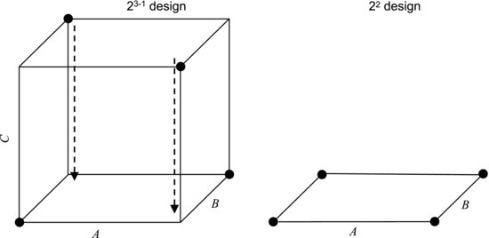
An interesting property of the half factorial design is that, if one factor turns out to be unimportant, the design collapses to a full factorial design. This is most easily understood looking at it graphically. The left part of Figure 9.8 shows a three-factor half factorial design. The dots in the corners show the treatments used and we see that every other treatment is missing from the corresponding full factorial design, which is represented by all the corners of the cube. If, for instance, factor C turns out not to have a significant effect on the response, this means that there is no discernible difference in the response when C is switched between its two levels. In other words, a change in the setting of C only measures the experimental error. This could be seen as the cube collapsing along the C-direction. As shown in the right-hand part of the figure, we then obtain a full factorial design with the remaining two factors A and B. If these factors turn out to be significant, we now have data for a more detailed study of them.

Figure 9.8 The three-factor half factorial design may collapse to a two-factor full factorial design if one factor (here C) turns out to be unimportant.

The fact that every other corner point is missing can be advantageous in other ways than just reducing the number of runs. In the corners, all factors are set to their extreme settings. In some cases it is not safe or even possible to run experiments at such extreme conditions. If we are worried about particular combinations of settings, these reduced designs allow us to choose a fraction of the runs that avoids these settings.

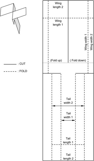
Now, let us run a real experiment to see how screening and analysis work in factorial experiments. You will design a paper helicopter, optimizing the settings of five factors in no more than 16 runs. The experiment should normally include at least one replicate but it is omitted in this example to limit your workload. The helicopter blueprint is shown in Figure 9.9. You should take photocopies and cut helicopters from them with a pair of scissors. The factors to be screened are the tail length, tail width, wing length, wing width and the weight. To keep the weight constant when varying the other factors you should cut along the solid lines and vary the factors by folding the paper along the appropriate dashed lines. This keeps the total amount of paper in the helicopter constant. The weight is manipulated by attaching a paper clip to the bottom of the body. Fold the wings in separate directions at the dotted line to obtain a “T”-shaped paper figure, as shown in the insert to the left of the blueprint. The response variable to be maximized is the flight time, so you will need a stopwatch. To fly the helicopter, hold the body between your thumb and index finger and drop it from a predetermined height.

Figure 9.9 Blueprint for the helicopter experiment. Take photocopies, cut along solid lines and fold along dashed ones.

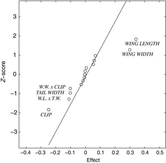
This method for designing and analyzing fractional factorial experiments can, of course, be extended to more factors and various fractions of a full factorial design. A lack in the design in Exercise 9.9 is that it does not include replicates. This is because we did not attempt to estimate the error explicitly. We can read the error from a normal plot as the one in Figure 9.10, which shows the results from one particular helicopter experiment. As described in Example 7.4, the line drawn through the upper and lower quartiles approximates the error. The slope shows that the effect changes by about 0.2 seconds in three standard deviations (Z-scores), giving us a standard deviation of about 0.07 s. The plot indicates that the length and width of the wings increases the flight time, whereas the clip decreases it. The tail width and two interactions plot slightly off the line but it is difficult to judge their importance.

If we were using regression modeling, as we will in the next section, replicates would be needed to provide extra degrees of freedom for estimating the error. Note that the replicates should include as many sources of uncertainty as possible, both from the “manufacture” and flying of the helicopter. With one replicate run this would require us to make two helicopters for each treatment.

Figure 9.10 Normal plot from a helicopter experiment.

Despite the lack of replicates, two important precautions were employed in this experiment: randomization and a fixed operating procedure. Needless to say, it is important to settle on a fixed drop height, a fixed method of releasing the helicopter, a predefined manner of counting down to the drop, appointing a single person to operate the timer, and so forth. To obtain a feeling for how shortcomings in the experimental procedure can influence the result it is useful to carry the exercise out in several teams and compare the outcomes. It is, for example, common to find that different teams have made the helicopters in slightly different ways, since even a detailed building instruction leaves room for interpretation. Make sure to fly the best helicopters from different teams using one operating procedure and then discuss how any differences may be explained. This exercise demonstrates the need for describing experimental procedures in great detail when publishing research results. The reader must be able to repeat both the experiment and the outcome.

Before ending this section we will briefly mention another class of screening designs, called Plackett–Burman designs. As we have seen, the number of treatments in fractional factorial designs is always a power of two: 4, 8, 16, 32, 64 and so on. The gaps between the numbers increase when the number of factors increases. With a very large number of factors it may be difficult to find a design of reasonable size. With Plackett–Burman designs the number of treatments is a multiple of four. For example, designs with 12, 20, 24 and 36 treatments can be obtained. This makes it easier to find a design that matches your experimental limitations. Just as factorial designs, Plackett–Burman designs are orthogonal matrices whose elements are all +1 or −1, but they are smaller. Technically, they are Hadamard matrices and you can find free libraries of them by searching the internet for “Plackett–Burman designs” or “Hadamard matrices”. Plackett–Burman experiments are analyzed analogously to factorial experiments. A drawback of these designs is that the main effects are confounded with two-way interactions. This means that, if there are important interactions in the system under study, these will be mistaken for main effects in the analysis. Considering that screening experiments are made because we do not know which factors and interactions are important, it is rarely a safe assumption that interactions do not exist. For this reason, Plackett–Burman designs should be applied with caution.