Chapter 11

Texture Mapping

When trying to replicate the look of the real world, one quickly realizes that hardly any surfaces are featureless. Wood grows with grain; skin grows with wrinkles; cloth shows its woven structure; paint shows the marks of the brush or roller that laid it down. Even smooth plastic is made with bumps molded into it, and smooth metal shows the marks of the machining process that made it. Materials that were once featureless quickly become covered with marks, dents, stains, scratches, fingerprints, and dirt.

In computer graphics we lump all these phenomena under the heading of “spatially varying surface properties”—attributes of surfaces that vary from place to place but don’t really change the shape of the surface in a meaningful way. To allow for these effects, all kinds of modeling and rendering systems provide some means for texture mapping : using an image, called a texture map , texture image , or just a texture , to store the details that you want to go on a surface, then mathematically “mapping” the image onto the surface.

As it turns out, once the mechanism to map images onto surfaces exists, there are many less obvious ways it can be used that go beyond the basic purpose of introducing surface detail. Textures can be used to make shadows and reflections, to provide illumination, even to define surface shape. In sophisticated interactive programs, textures are used to store all kinds of data that doesn’t even have anything to do with pictures!

This chapter discusses the use of texture for representing surface detail, shadows, and reflections. While the basic ideas are simple, several practical problems complicate the use of textures. First of all, textures easily become distorted, and designing the functions that map textures onto surfaces is challenging. Also, texture mapping is a resampling process, just like rescaling an image, and as we saw in Chapter 9, resampling can very easily introduce aliasing artifacts. The use of texture mapping and animation together readily produces truly dramatic aliasing, and much of the complexity of texture mapping systems is created by the antialiasing measures that are used to tame these artifacts.

11.1 Looking Up Texture Values

To start off, let’s consider a simple application of texture mapping. We have a scene with a wood floor, and we would like the diffuse color of the floor to be controlled by an image showing floorboards with wood grain. Regardless of whether we are using ray tracing or rasterization, the shading code that computes the color for a ray-surface intersection point or for a fragment generated by the rasterizer needs to know the color of the texture at the shading point, in order to use it as the diffuse color in the Lambertian shading model from Chapter 10.

To get this color, the shader performs a texture lookup: it figures out the location, in the coordinate system of the texture image, that corresponds to the shading point, and it reads out the color at that point in the image, resulting in the texture sample . That color is then used in shading, and since the texture lookup happens at a different place in the texture for every pixel that sees the floor, a pattern of different colors shows up in the image. The code might look like this:

Color texture_lookup(Texture t, float u, float v) {

   int i = round(u * t.width() - 0.5)

   int j = round(v * t.height() - 0.5)

   return t.get_pixel(i,j)

}

Color shade_surface_point(Surface s, Point p, Texture t) {

   Vector normal = s.get_normal(p)

   (u,v) = s.get_texcoord(p)

   Color diffuse_color = texture_lookup(u,v)

   // compute shading using diffuse_color and normal

   // return shading result

}

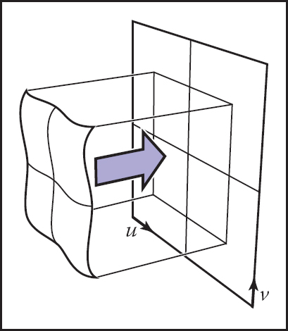
In this code, the shader asks the surface where to look in the texture, and somehow every surface that we want to shade using a texture needs to be able to answer this query. This brings us to the first key ingredient of texture mapping: we need a function that maps from the surface to the texture that we can easily compute for every pixel. This is the texture coordinate function (Figure 11.1) and we say that it assigns texture coordinates to every point on the surface. Mathematically it is a mapping from the surface S to the domain of the texture, T:

$\begin{array}{l}\varphi :S\to T\\ :\left(x,y,z\right)\mapsto \left(u,v\right).\end{array}$

The set T, often called “texture space,” is usually just a rectangle that contains the image; it is common to use the unit square (u, v) ∈ [0, 1]2 (in this book we’ll use the names u and v for the two texture coordinates). In many ways it’s similar to the viewing projection discussed in Chapter 7, called π in this chapter, which maps points on surfaces in the scene to points in the image; both are 3D-to-2D mappings, and both are needed for rendering—one to know where to get the texture value from, and one to know where to put the shading result in the image. But there are some important differences, too: π is almost always a perspective or orthographic projection, whereas ϕ can take on many forms; and there is only one viewing projection for an image, whereas each object in the scene is likely to have a completely separate texture coordinate function.

It may seem surprising that ϕ is a mapping from the surface to the texture, when our goal is to put the texture onto the surface, but this is the function we need.

For the case of the wood floor, if the floor happens to be at constant z and aligned to the x and y axes, we could just use the mapping

$u=ax;v=by,$

for some suitably chosen scale factors a and b, to assign texture coordinates (s, t) to the point (x, y, z)floor, and then use the value of the texture pixel, or texel, closest to (u, v) as the texture value at (x, y). In this way we rendered the image in Figure 11.2.

This is pretty limiting, though: what if the room is modeled at an angle to the x and y axes, or what if we want the wood texture on the curved back of a chair? We will need some better way to compute texture coordinates for points on the surface.

Another problem that arises from the simplest form of texture mapping is illustrated dramatically by rendering at a high contrast texture from a very grazing angle into a low-resolution image. Figure 11.3 shows a larger plane textured using the same approach but with a high contrast grid pattern and a view toward the horizon. You can see it contains aliasing artifacts (stairsteps in the foreground, wavy and glittery patterns in the distance) similar to the ones that arise in image resampling (Chapter 9) when appropriate filters are not used. Although it takes an extreme case to make these artifacts so obvious in a tiny still image printed in a book, in animations these patterns move around and are very distracting even when they are much more subtle.

We have now seen the two primary issues in basic texture mapping:

• defining texture coordinate functions, and
• looking up texture values without introducing too much aliasing.

These two concerns are fundamental to all kinds of applications of texture mapping and are discussed in Sections 11.2 and 11.3. Once you understand them and some of the solutions to them, then you understand texture mapping. The rest is just how to apply the basic texturing machinery for a variety of different purposes, which is discussed in Section 11.4.

11.2 Texture Coordinate Functions

Designing the texture coordinate function ϕ well is a key requirement for getting good results with texture mapping. You can think of this as deciding how you are going to deform a flat, rectangular image so that it conforms to the 3D surface you want to draw. Or alternatively, you are taking the surface and gently flattening it, without letting it wrinkle, tear, or fold, so that it lies flat on the image. Sometimes this is easy: maybe the 3D surface is already a flat rectangle! In other cases it’s very tricky: the 3D shape might be very complicated, like the surface of a character’s body.

The problem of defining texture coordinate functions is not new to computer graphics. Exactly the same problem is faced by cartographers when designing maps that cover large areas of the Earth’s surface: the mapping from the curved globe to the flat map inevitably causes distortion of areas, angles, and/or distances that can easily make maps very misleading. Many map projections have been proposed over the centuries, all balancing the same competing concerns—of minimizing various kinds of distortion while covering a large area in one contiguous piece—that are faced in texture mapping.

In some applications (as we’ll see later in this chapter) there’s a clear reason to use a particular map. But in most cases, designing the texture coordinate map is a delicate task of balancing competing concerns, which skilled modelers put considerable effort into.

You can define ϕ in just about any way you can dream up. But there are several competing goals to consider:

• Bijectivity. In most cases you’d like ϕ to be bijective (see Section 2.1.1), so that each point on the surface maps to a different point in texture space. If several points map to the same texture space point, the value at one point in the texture will affect several points on the surface. In cases where you want a texture to repeat over a surface (think of wallpaper or carpet with their repeating patterns), it makes sense to deliberately introduce a many-to-one mapping from surface points to texture points, but you don’t want this to happen by accident.
• Size distortion. The scale of the texture should be approximately constant across the surface. That is, close-together points anywhere on the surface that are about the same distance apart should map to points about the same distance apart in the texture. In terms of the function ϕ , the magnitude of the derivatives of ϕ should not vary too much.
• Shape distortion. The texture should not be very distorted. That is, a small circle drawn on the surface should map to a reasonably circular shape in texture space, rather than an extremely squashed or elongated shape. In terms of ϕ , the derivative of ϕ should not be too different in different directions.
• Continuity. There should not be too many seams: neighboring points on the surface should map to neighboring points in the texture. That is, ϕ should be continuous, or have as few discontinuities as possible. In most cases, some discontinuities are inevitable, and we’d like to put them in inconspicuous locations.

Surfaces that are defined by parametric equations (Section 2.5.8) come with a built-in choice for the texture coordinate function: simply invert the function that defines the surface, and use the two parameters of the surface as texture coordinates. These texture coordinates may or may not have desirable properties, depending on the surface, but they do provide a mapping.

But for surfaces that are defined implicitly, or are just defined by a triangle mesh, we need some other way to define the texture coordinates, without relying on an existing parameterization. Broadly speaking, the two ways to define texture coordinates are to compute them geometrically, from the spatial coordinates of the surface point, or, for mesh surfaces, to store values of the texture coordinates at vertices and interpolate them across the surface. Let’s look at these options one at a time.

11.2.1 Geometrically Determined Coordinates

Geometrically determined texture coordinates are used for simple shapes or special situations, as a quick solution, or as a starting point for designing a hand-tweaked texture coordinate map.

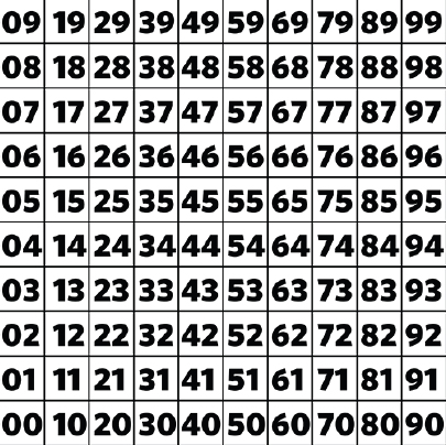
We will illustrate the various texture coordinate functions by mapping the test image in Figure 11.4 onto the surface. The numbers in the image let you read the approximate (u, v) coordinates out of the rendered image, and the grid lets you see how distorted the mapping is.

Planar Projection

Probably the simplest mapping from 3D to 2D is a parallel projection—the same mapping as used for orthographic viewing (Figure 11.5). The machinery we developed already for viewing (Section 7.1) can be re-used directly for defining texture coordinates: just as orthographic viewing boils down to multiplying by a matrix and discarding the z component, generating texture coordinates by planar projection can be done with a simple matrix multiply:

$\varphi \left(x,y,z\right)=\left(u,v\right)\text{where}\left[\begin{array}{l}u\\ v\\ *\\ 1\end{array}\right]=M_t\left[\begin{array}{l}x\\ y\\ z\\ 1\end{array}\right],$

where the texturing matrix Mt represents an affine transformation, and the asterisk indicates that we don’t care what ends up in the third coordinate.

This works quite well for surfaces that are mostly flat, without too much variation in surface normal, and a good projection direction can be found by taking the average normal. For any kind of closed shape, though, a planar projection will not be injective: points on the front and back will map to the same point in texture space (Figure 11.6).

By simply substituting perspective projection for orthographic, we get projective texture coordinates (Figure 11.7):

$\varphi \left(x,y,z\right)=\left(\tilde{u}/w,\tilde{v}/w\right)\text{where}\left[\begin{array}{l}\tilde{u}\\ \tilde{v}\\ *\\ w\end{array}\right]=P_t\left[\begin{array}{l}x\\ y\\ z\\ 1\end{array}\right].$

Now the 4 × 4 matrix Pt represents a projective (not necessarily affine) transformation—that is, the last row may not be [0, 0,0,1].

Projective texture coordinates are important in the technique of shadow mapping, discussed in Section 11.4.4.

Spherical Coordinates

For spheres, the latitude/longitude parameterization is familiar and widely used. It has a lot of distortion near the poles, which can lead to difficulties, but it does cover the whole sphere with discontinuities only along one line of latitude.

Surfaces that are roughly spherical in shape can be parameterized using a texture coordinate function that maps a point on the surface to a point on a sphere using radial projection: take a line from the center of the sphere through the point on the surface, and find the intersection with the sphere. The spherical coordinates of this intersection point are the texture coordinates of the point you started with on the surface.

Another way to say this is that you express the surface point in spherical coordinates (ρ θ, ϕ) and then discard the ρ coordinate and map θ and ϕ each to the range [0,1]. The formula depends on the spherical coordinates convention; using the convention of Section 2.5.8,

$\varphi \left(x,y,z\right)=\left(\left[\pi +\text{atan}2\left(y,x\right)\right]/2\pi ,\left[\pi -\text{acos}\left(\text{z/}||x||\right)\right]/\pi \right).$

A spherical coordinates map will be bijective everywhere except at the poles if the whole surface is visible from the center point. It inherits the same distortion near the poles as the latitude-longitude map on the sphere. Figure 11.8 shows an object for which spherical coordinates provide a suitable texture coordinate function.

Cylindrical Coordinates

For objects that are more columnar than spherical, projection outward from an axis onto a cylinder may work better than projection from a point onto a sphere (Figure 11.9). Analogously to spherical projection, this amounts to converting to cylindrical coordinates and discarding the radius:

$\varphi \left(x,y,z\right)=\left(\frac{1}{2\pi }\left[\pi +\text{atan}2\left(y,x\right)\right]/2\pi ,\frac{1}{2}\left[1+z\right]\right).$

Cubemaps

Using spherical coordinates to parameterize a spherical or sphere-like shape leads to high distortion of shape and area near the poles, which often leads to visible artifacts that reveal that there are two special points where something is going wrong with the texture. A popular alternative is much more uniform at the cost of having more discontinuities. The idea is to project onto a cube, rather than a sphere, and then use six separate square textures for the six faces of the cube. The collection of six square textures is called a cubemap. This introduces discontinuities along all the cube edges, but it keeps distortion of shape and area low.

Computing cubemap texture coordinates is also cheaper than for spherical coordinates, because projecting onto a plane just requires a division—essentially the same as perspective projection for viewing. For instance, for a point that projects onto the +z face of the cube:

$\left(x,y,z\right)\mapsto \left(\frac{x}{z},\frac{y}{z}\right).$

A confusing aspect of cubemaps is establishing the convention for how the u and v directions are defined on the six faces. Any convention is fine, but the convention chosen affects the contents of textures, so standardization is important. Because cubemaps are very often used for textures that are viewed from the inside of the cube (see environment mapping in Section 11.4.5), the usual conventions have the u and v axes oriented so that u is clockwise from v as viewed from inside. The convention used by OpenGL is

$\begin{array}{l}{\varphi }_{-x}\left(x,y,z\right)=\frac{1}{2}\left[1+\left(+z,-y\right)/\left|x\right|\right],\\ {\varphi }_{+x}\left(x,y,z\right)=\frac{1}{2}\left[1+\left(-z,-y\right)/\left|x\right|\right],\\ {\varphi }_{-y}\left(x,y,z\right)=\frac{1}{2}\left[1+\left(+x,-z\right)/\left|y\right|\right],\\ {\varphi }_{+y}\left(x,y,z\right)=\frac{1}{2}\left[1+\left(+x,+z\right)/\left|y\right|\right],\\ {\varphi }_{-z}\left(x,y,z\right)=\frac{1}{2}\left[1+\left(-x,-z\right)/\left|z\right|\right],\\ {\varphi }_{+z}\left(x,y,z\right)=\frac{1}{2}\left[1+\left(+x,-y\right)/\left|z\right|\right].\end{array}$

The subscripts indicate which face of the cube each projection corresponds to. For example, cItalic">ϕ−x is used for points that project to the face of the cube at x = +1. You can tell which face a point projects to by looking at the coordinate with the largest absolute value: for example, if |x| < |y| and |x| > |z|, the point projects to the +x or −x face, depending on the sign of x.

A texture to be used with a cube map has six square pieces. (See Figure 11.10.) Often they are packed together in a single image for storage, arranged as if the cube was unwrapped.

11.2.2 Interpolated Texture Coordinates

For more fine-grained control over the texture coordinate function on a triangle mesh surface, you can explicitly store the texture coordinates at each vertex, and interpolate them across the triangles using barycentric interpolation (Section 8.1.2). It works in exactly the same way as any other smoothly varying quantities you might define over a mesh: colors, normals, even the 3D position itself.

Let’s look at an example with a single triangle. Figure 11.11 shows a triangle texture mapped with part of the by now familiar test pattern. By looking at the pattern that appears on the rendered triangle, you can deduce that the texture coordinates of the three vertices are (0.2, 0.2), (0.8, 0.2), and (0.2, 0.8), because those are the points in the texture that appear at the three corners of the triangle. Just as with the geometrically determined mappings in the previous section, we control where the texture goes on the surface by giving the mapping from the surface to the texture domain, in this case by specifying where each vertex should go in texture space. Once you position the vertices, linear (barycentric) interpolation across triangles takes care of the rest.

In Figure 11.12 we show a common way to visualize texture coordinates on a whole mesh: simply draw triangles in texture space with the vertices positioned at their texture coordinates. This visualization shows you what parts of the texture are being used by which triangles, and it is a handy tool for evaluating texture coordinates and for debugging all sorts of texture-mapping code.

The quality of a texture coordinate mapping that is defined by vertex texture coordinates depends on what coordinates are assigned to the vertices—that is, how the mesh is laid out in texture space. No matter what coordinates are assigned, as long as the triangles in the mesh share vertices (Section 12.1), the texture coordinate mapping is always continuous, because neighboring triangles will agree on the texture coordinate at points on their shared edge. But the other desirable qualities described above are not so automatic. Injectivity means the triangles don’t overlap in texture space—if they do, it means there’s some point in the texture that will show up at more than one place on the surface.

Size distortion is low when the areas of triangles in texture space are in proportion to their areas in 3D. For instance, if a character’s face is mapped with a continuous texture coordinate function, one often ends up with the nose squeezed into a relatively small area in texture space, as shown in Figure 11.13. Although triangles on the nose are smaller than on the cheek, the ratio of sizes is more extreme in texture space. The result is that the texture is enlarged on the nose, because a small area of texture has to cover a large area of surface. Similarly, comparing the forehead to the temple, the triangles are similar in size in 3D, but the triangles around the temple are larger in texture space, causing the texture to appear smaller there.

Similarly, shape distortion is low when the shapes of triangles are similar in 3D and in texture space. The face example has fairly low shape distortion, but, for example, the sphere in Figure 11.17 has very large shape distortion near the poles.

11.2.3 Tiling, Wrapping Modes, and Texture Transformations

It’s often useful to allow texture coordinates to go outside the bounds of the texture image. Sometimes this is a detail: rounding error in a texture coordinate calculation might cause a vertex that lands exactly on the texture boundary to be slightly outside, and the texture mapping machinery should not fail in that case. But it can also be a modeling tool.

If a texture is only supposed to cover part of the surface, but texture coordinates are already set up to map the whole surface to the unit square, one option is to prepare a texture image that is mostly blank with the content in a small area. But that might require a very high resolution texture image to get enough detail in the relevant area. Another alternative is to scale up all the texture coordinates so that they cover a larger range—[−4.5, 5.5] × [−4.5, 5.5] for instance, to position the unit square at one-tenth size in the center of the surface.

For a case like this, texture lookups outside the unit-square area that’s covered by the texture image should return a constant background color. One way to do this is to set a background color to be returned by texture lookups outside the unit square. If the texture image already has a constant background color (for instance, a logo on a white background), another way to extend this background automatically over the plane is to arrange for lookups outside the unit square to return the color of the texture image at the closest point on the edge, achieved by clamping the u and v coordinates to the range from the first pixel to the last pixel in the image.

Sometimes we want a repeating pattern, such as a checkerboard, a tile floor, or a brick wall. If the pattern repeats on a rectangular grid, it would be wasteful to create an image with many copies of the same data. Instead we can handle texture lookups outside the texture image using wraparound indexing—when the lookup point exits the right edge of the texture image, it wraps around to the left edge. This is handled very simply using the integer remainder operation on the pixel coordinates.

Color texture_lookup_wrap(Texture t, float u, float v) {

   int i = round(u * t.width() - 0.5)

   int j = round(v * t.height() - 0.5)

   return t.get_pixel(i % t.width(), j % t.height())

}

Color texture_lookup_wrap(Texture t, float u, float v) {

   int i = round(u * t.width() - 0.5)

   int j = round(v * t.height() - 0.5)

   return t.get_pixel(max(0, min(i, t.width()-1)),

    (max(0, min(j, t.height()-1))))

}

The choice between these two ways of handling out-of-bounds lookups is specified by selecting a wrapping mode from a list that includes tiling, clamping, and often combinations or variants of the two. With wrapping modes, we can freely think of a texture as a function that returns a color for any point in the infinite 2D plane (Figure 11.14). When we specify a texture using an image, these modes describe how the finite image data is supposed to be used to define this function. In Section 11.5, we’ll see that procedural textures can naturally extend across an infinite plane, since they are not limited by finite image data. Since both are logically infinite in extent, the two types of textures are interchangeable.

When adjusting the scale and placement of textures, it’s convenient to avoid actually changing the functions that generate texture coordinates, or the texture coordinate values stored at vertices of meshes, by instead applying a matrix trans formation to the texture coordinates before using them to sample the texture:

$\varphi \left(x\right)=M_T={\varphi }_{\text{model}}\left(x\right),$

where ϕmodel is the texture coordinate function provided with the model, and MT is a 3 by 3 matrix representing an affine or projective transformation of the 2D texture coordinates using homogeneous coordinates. Such a transformation, sometimes limited just to scaling and/or translation, is supported by most renderers that use texture mapping.

11.2.4 Perspective Correct Interpolation

There are some subtleties in achieving correct-looking perspective by interpolating texture coordinates across triangles, but we can address this at the rasterization stage. The reason things are not straightforward is that just interpolating texture coordinates in screen space results in incorrect images, as shown for the grid texture in Figure 11.15. Because things in perspective get smaller as the distance to the viewer increases, the lines that are evenly spaced in 3D should compress in 2D image space. More careful interpolation of texture coordinates is needed to accomplish this.

We can implement texture mapping on triangles by interpolating the (u, v) coordinates, modifying the rasterization method of Section 8.1.2, but this results in the problem shown at the right of Figure 11.15. A similar problem occurs for triangles if screen space barycentric coordinates are used as in the following rasterization code:

for all x do

  for all y do

  compute (α, β, γ) for (x, y)

  if α ∈ (0,1) and β ∈ (0,1) and γ ∈ (0,1) then

  t = α t0 + βt1 + γt2

  drawpixel (x, y) with color texture(t) for a solid texture

  or with texture(β, γ) for a 2D texture.

This code will generate images, but there is a problem. To unravel the basic problem, let’s consider the progression from world space q to homogeneous point r to homogenized point s:

$\left[\begin{array}{l}{x}_q\\ y_q\\ z_q\\ 1\end{array}\right]\underrightarrow{\text{transform}}\left[\begin{array}{l}{x}_r\\ y_r\\ z_r\\ h_r\end{array}\right]\underrightarrow{\text{homogenize}}\left[\begin{array}{l}{x}_r/h_r\\ y_r/h_r\\ z_r/h_r\\ 1\end{array}\right]\equiv \left[\begin{array}{l}{x}_s\\ y_s\\ z_s\\ 1\end{array}\right].$

The simplest form of the texture coordinate interpolation problem is when we have texture coordinates (u, v) associated with two points, q and Q, and we need to generate texture coordinates in the image along the line between s and S. If the world-space point q′ that is on the line between q and Q projects to the screen-space point s′ on the line between s and S, then the two points should have the same texture coordinates.

The naïve screen-space approach, embodied by the algorithm above, says that at the point s' = s + α (S − s) we should use texture coordinates us + α(uS - us) and vs + α(vS -vs). This doesn’t work correctly because the world-space point q' that transforms to s' is not q + α (Q − q).

However, we know from Section 7.4 that the points on the line segment between q and Q do end up somewhere on the line segment between s and S; in fact, in that section we showed that

$q+t\left(Q-q\right)\mapsto s+\alpha \left(S+s\right).$

The interpolation parameters t and α are not the same, but we can compute one from the other:1

$t\left(\alpha \right)=\frac{w_r\alpha }{w_R+\alpha \left(w_r-w_R\right)}\text{and}\alpha \left(t\right)=\frac{w_{R}t}{w_r+t\left(w_R-w_r\right)}.\text{ (11.1)}$

These equations provide one possible fix to the screen-space interpolation idea. To get texture coordinates for the screen-space point s′ = s + α (S − s), compute u's = us+t (α)(uS − us) and v's = vs +t (α)(vS −vs). These are the coordinates of the point q′ that maps to s', so this will work. However, it is slow to evaluate t(α) for each fragment, and there is a simpler way.

The key observation is that because, as we know, the perspective transform preserves lines and planes, it is safe to linearly interpolate any attributes we want across triangles, but only as long as they go through the perspective transformation along with the points. To get a geometric intuition for this, reduce the dimension so that we have homogeneous points (xr,yr,wr) and a single attribute u being interpolated. The attribute u is supposed to be a linear function of xr and yr, so if we plot u as a height field over (xr,yr) the result isa plane. Now, if we think of u as a third spatial coordinate (call it ur to emphasize that it’s treated the same as the others) and send the whole 3D homogeneous point (xr,yr,ur,wr) through the perspective transformation, the result (xs,ys,us) still generates points that lie on a plane. There will be some warping within the plane, but the plane stays flat. This means that us is a linear function of (xs, ys)—which is to say, we can compute us anywhere by using linear interpolation based on the coordinates (xs,ys).

Returning to the full problem, we need to interpolate texture coordinates (u,v) that are linear functions of the world space coordinates (xq, yq,zq). After transforming the points to screen space, and adding the texture coordinates as if they were additional coordinates, we have

$\left[\begin{array}{l}u\\ v\\ 1\\ x_r\\ y_r\\ z_r\\ w_r\end{array}\right]\underrightarrow{\text{homogenize}}\left[\begin{array}{l}u/w_r\\ v/w_r\\ 1/w_r\\ x_r/w_r=x_s\\ y_r/w_r=y_s\\ z_r/w_r=z_s\\ 1\end{array}\right].\text{ (11.2)}$

The practical implication of the previous paragraph is that we can go ahead and interpolate all of these quantities based on the values of (xs, ys)—including the value zs, used in the z-buffer. The problem with the naïve approach is simply that we are interpolating components selected inconsistently—as long as the quantities involved are from before or all from after the perspective divide, all will be well.

The one remaining problem is that (u/wr, v/wr) is not directly useful for looking up texture data; we need (u, v). This explains the purpose of the extra parameter we slipped into (11.2), whose value is always 1: once we have u/wr, v/wr, and 1/wr, we can easily recover (u, v) by dividing.

To verify that this is all correct, let’s check that interpolating the quantity 1/wr in screen space indeed produces the reciprocal of the interpolated wr in world space. To see this is true, confirm (Exercise 2):

$\frac{1}{w_r}+\alpha \left(t\right)\left(\frac{1}{w_R}-\frac{1}{w_r}\right)=\frac{1}{{w^{\prime }}_r}=\frac{1}{w_r+t\left(w_R-w_r\right)}\text{ (11.3)}$

remembering that α(t) and t are related by Equation 11.1.

This ability to interpolate 1/wr linearly with no error in the transformed space allows us to correctly texture triangles. We can use these facts to modify our scan-conversion code for three points ti = (xi, yi, zi, wi) that have been passed through the viewing matrices, but have not been homogenized, complete with texture coordinates ti = (ui, vi):

for all xs do

 for all ys do

 compute (α, β, γ) for (xs, ys)

 if (α ∈ [0,1] and β ∈ [0,1] and γ ∈ [0,1]) then

   us = α (u 0/w 0) +β (u 1/w 1) + γ (u 2/w 2)

   vs = α (v 0/w 0) + β (v 1/w 1) + γ (v 2/w 2)

   1s = α(1/w 0) + β(1/w 1) + γ (2/w 2)

   u = us/1s

   v = vs/1s

   drawpixel (xs, ys) with color texture(u, v)

Of course, many of the expressions appearing in this pseudocode would be precomputed outside the loop for speed. For solid textures, it’s simple enough to include the original world space coordinates xq,yq, zq in the list of attributes, treated the same as u and v, and correct interpolated world space coordinates will be obtained, which can be passed to the solid texture function.

11.2.5 Continuity and Seams

Although low distortion and continuity are nice properties to have in a texture coordinate function, discontinuities are often unavoidable. For any closed 3D surface, it’s a basic result of topology that there is no continuous, bijective function that maps the whole surface into a texture image. Something has to give, and by introducing seams—curves on the surface where the texture coordinates change suddenly—we can have low distortion everywhere else. Many of the geometrically determined mappings discussed above already contain seams: in spherical and cylindrical coordinates, the seams are where the angle computed by atan2 wraps around from π to π, and in the cubemap, the seams are along the cube edges, where the mapping switches between the six square textures.

With interpolated texture coordinates, seams require special consideration, because they don’t happen naturally. We observed earlier that interpolated texture coordinates are automatically continuous on shared-vertex meshes—the sharing of texture coordinates guarantees it. But this means that if a triangle spans a seam, with some vertices on one side and some on the other, the interpolation machinery will cheerfully provide a continuous mapping, but it will likely be highly distorted or fold over so that it’s not injective. Figure 11.17 illustrates this problem on a globe mapped with spherical coordinates. For example, there is a triangle near the bottom of the globe that has one vertex at the tip of New Zealand’s South Island, and another vertex in the Pacific about 400 km northeast of the North Island. A sensible pilot flying between these points would fly over New Zealand, but the path starts at longitude 167°s E (+167) and ends at 179°s W (that is, longitude −179), so linear interpolation chooses a route that crosses South America on the way. This causes a backward copy of the entire map to be compressed into the strip of triangles that crosses the 180th meridian! The solution is to label the second vertex with the equivalent longitude of 181°s E, but this just pushes the problem to the next triangle.

The only way to create a clean transition is to avoid sharing texture coordinates at the seam: the triangle crossing New Zealand needs to interpolate to longitude +181, and the next triangle in the Pacific needs to continue starting from to longitude −179. To do this, we duplicate the vertices at the seam: for each vertex we add a second vertex with an equivalent longitude, differing by 360°s, and the triangles on opposite sides of the seam use different vertices. This solution is shown in the right half of Figure 11.17, in which the vertices at the far left and right of the texture space are duplicates, with the same 3D positions.

11.3 Antialiasing Texture Lookups

The second fundamental problem of texture mapping is antialiasing. Rendering a texture mapped image is a sampling process: mapping the texture onto the surface and then projecting the surface into the image produces a 2D function across the image plane, and we are sampling it at pixels. As we saw in Chapter 9, doing this using point samples will produce aliasing artifacts when the image contains detail or sharp edges—and since the whole point of textures is to introduce detail, they become a prime source of aliasing problems like the ones we saw in Figure 11.3.

Just as with antialiased rasterization of lines or triangles, antialiased ray tracing (Section 13.4), or downsampling images (Section 9.4), the solution is to make each pixel not a point sample but an area average of the image, over an area similar in size to the pixel. Using the same supersampling approach used for antialiased rasterization and ray tracing, with enough samples, excellent results can be obtained with no changes to the texture mapping machinery: many samples within a pixel’s area will land at different places in the texture map, and averaging the shading results computed using the different texture lookups is an accurate way to approximate the average color of the image over the pixel. However, with detailed textures it takes very many samples to get good results, which is slow. Computing this area average efficiently in the presence of textures on the surface is the first key topic in texture antialiasing.

Texture images are usually defined by raster images, so there is also a reconstruction problem to be considered, just as with upsampling images (Section 9.4). The solution is the same for textures: use a reconstruction filter to interpolate between texels.

We expand on each of these topics in the following sections.

11.3.1 The Footprint of a Pixel

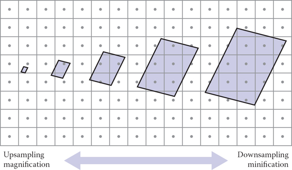
What makes antialiasing textures more complex than other kinds of antialiasing is that the relationship between the rendered image and the texture is constantly changing. Every pixel value should be computed as an average color over the area belonging to the pixel in the image, and in the common case that the pixel is looking at a single surface, this corresponds to averaging over an area on the surface. If the surface color comes from a texture, this in turn amounts to averaging over a corresponding part of the texture, known as the texture space footprint of the pixel. Figure 11.18 illustrates how the footprints of square areas (which could be pixel areas in a lower-resolution image) map to very different sized and shaped areas in the floor’s texture space.

Recall the three spaces involved in rendering with textures: the projection π that maps 3D points into the image and the texture coordinate function ϕ that maps 3D points into texture space. To work with pixel footprints we need to understand the composition of these two mappings: first follow π backwards to get from the image to the surface, then follow ϕ forwards. This composition ψ = ϕ ∘ π−1is what determines pixel footprints: the footprint of a pixel is the image of that pixel’s square area of the image under the mapping ψ.

The core problem in texture antialiasing is computing an average value of the texture over the footprint of a pixel. To do this exactly in general could be a pretty complicated job: for a faraway object with a complicated surface shape, the footprint could be a complicated shape covering a large area, or possibly several disconnected areas, in texture space. But in the typical case, a pixel lands in a smooth area of surface that is mapped to a single area in the texture.

Because ψ contains both the mapping from image to surface and the mapping from surface to texture, the size and shape of the footprint depend on both the viewing situation and the texture coordinate function. When a surface is closer to the camera, pixel footprints will be smaller; when the same surface moves farther away, the footprint gets bigger. When surfaces are viewed at an oblique angle, the footprint of a pixel on the surface is elongated, which usually means it will be elongated in texture space also. Even with a fixed view, the texture coordinate function can cause variations in the footprint: if it distorts area, the size of footprints will vary, and if it distorts shape, they can be elongated even for head-on views of the surface.

However, to find an efficient algorithm for computing antialiased lookups, some substantial approximations will be needed. When a function is smooth, a linear approximation is often useful. In the case of texture antialiasing, this means approximating the mapping ψ from image space to texture space as a linear mapping from 2D to 2D:

$\psi \left(x\right)=\psi \left(x_{\text{0}}\right)+J\left(x-x_{\text{0}}\right),$

where the 2-by-2 matrix J is some approximation to the derivative of ψ. It has four entries, and if we denote the image-space position as x = (x, y) and the texture-space position as u = (u, v) then

$M=\left[\begin{array}{ll}\frac{du}{dx}\hfill & \frac{du}{dy}\hfill \\ \frac{dv}{dx}\hfill & \frac{dv}{dy}\hfill \end{array}\right],$

where the four derivatives describe how the texture point (u, v) that is seen at a point (x, y) in the image changes when we change x and y.

A geometric interpretation of this approximation is that it says a unit-sized square pixel area centered at x in the image will map approximately to a parallelogram in texture space, centered at ψ(x) and with its edges parallel to the vectors ux = (du/dx, dv/dx) and uy = (du/dy, dv/dy).

The derivative matrix J is useful because it tells the whole story of variation in the (approximated) texture-space footprint across the image. Derivatives that are larger in magnitude indicate larger texture-space footprints, and the relationship between the derivative vectors ux and uy indicates the shape. When they are orthogonal and the same length, the footprint is square, and as they become skewed and/or very different in length, the footprint becomes elongated.

We’ve now reached the form of the problem that’s usually thought of as the “right answer”: a filtered texture sample at a particular image-space position should be the average value of the texture map over the parallelogram-shaped footprint defined by the texture coordinate derivatives at that point. This already has some assumptions baked into it—namely, that the mapping from image to texture is smooth—but it is sufficiently accurate for excellent image quality. However, this parallelogram area average is already too expensive to compute exactly, so various approximations are used. Approaches to texture antialiasing differ in the speed/quality tradeoffs they make in approximating this lookup. We discuss these in the following sections.

11.3.2 Reconstruction

When the footprint is smaller than a texel, we are magnifying the texture as it is mapped into the image. This case is analogous to upsampling an image, and the main consideration is interpolating between texels to produce a smooth image in which the texel grid is not obvious. Just as in image upsampling, this smoothing process is defined by a reconstruction filter that is used to compute texture samples at arbitrary locations in texture space. (See Figure 11.20.)

The considerations are pretty much the same as in image resampling, with one important difference. In image resampling, the task is to compute output samples on a regular grid, and that regularity enabled an important optimization in the case of a separable reconstruction filter. In texture filtering, the pattern of lookups is not regular, and the samples have to be computed separately. This means large, high-quality reconstruction filters are very expensive to use, and for this reason the highest-quality filter normally used for textures is bilinear interpolation.

The calculation of a bilinearly interpolated texture sample is the same as computing one pixel in an image being upsampled with bilinear interpolation. First we express the texture-space sample point in terms of (real-valued) texel coordinates, then we read the values of the four neighboring texels and average them. Textures are usually parameterized over the unit square, and the texels are located in the same way as pixels in any image, spaced a distance 1/nu apart in the u direction and 1/nv in v , with texel (0,0) positioned half a texel in from the edge for symmetry. (See Chapter 9 for the full explanation.)

Color tex_sample_bilinear(Texture t, float u, float v) {

 u_p = u * t.width - 0.5

 v_p = v * t.height - 0.5

 iu0 = floor(u_p); iu1 = iu0 + 1

 iv0 = floor(v_p); iv1 = iv0 + 1

 a_u = (iu1 - u_p); b_u = 1 - a_u

 a_v = (iv1 - v_p); b_v = 1 - a_v

 return a_u * a_v * t[iu0][iv0] + a_u * b_v * t[iu0][iv1] +

  b_u * a_v * t[iu1][iv0] + b_u * b_v * t[iu1][iv1]

}

In many systems, this operation becomes an important performance bottleneck, mainly because of the memory latency involved in fetching the four texel values from the texture data. The pattern of sample points for textures is irregular, because the mapping from image to texture space is arbitrary, but often coherent, since nearby image points tend to map to nearby texture points that may read the same texels. For this reason, high-performance systems have special hardware devoted to texture sampling that handles interpolation and manages caches of recently used texture data to minimize the number of slow data fetches from the memory where the texture data is stored.

After reading Chapter 9 you may complain that linear interpolation may not be a smooth enough reconstruction for some demanding applications. However, it can always be made good enough by resampling the texture to a somewhat higher resolution using a better filter, so that the texture is smooth enough that bilinear interpolation works well.

11.3.3 Mipmapping

Doing a good job of interpolation only suffices in situations where the texture is being magnified: where the pixel footprint is small compared to the spacing of texels. When a pixel footprint covers many texels, good antialiasing requires computing the average of many texels to smooth out the signal so that it can be sampled safely.

One very accurate way to compute the average texture value over the footprint would be to find all the texels within the footprint and add them up. However, this is potentially very expensive when the footprint is large—it could require reading many thousands of texel just for a single lookup. A better approach is to precompute and store the averages of the texture over various areas of different size and position.

A very popular version of this idea is known as “MIP mapping” or just mipmapping. A mipmap is a sequence of textures that all contain the same image but at lower and lower resolution. The original, full-resolution texture image is called the base level , or level 0, of the mipmap, and level 1 is generated by taking that image and downsampling it by a factor of 2 in each dimension, resulting in an image with one-fourth as many texels. The texels in this image are, roughly speaking, averages of square areas 2 by 2 texels in size in the level-0 image.

This process can be continued to define as many mipmap levels as desired: the image at level k is computed by downsampling the image at level k − 1 by two. A texel at level k corresponds to a square area measuring 2k by 2k texels in the original texture. For instance, starting with a 1024 × 1024 texture image, we could generate a mipmap with 11 levels: level 0 is 1024 × 1024; level 1 is 512 × 512, and so on until level 10, which has just a single texel. This kind of structure, with images that represent the same content at a series of lower and lower sampling rates, is called an image pyramid , based on the visual metaphor of stacking all the smaller images on top of the original.

11.3.4 Basic Texture Filtering with Mipmaps

With the mipmap, or image pyramid, in hand, texture filtering can be done much more efficiently than by accessing many texels individually. When we need a texture value averaged over a large area, we simply use values from higher levels of the mipmap, which are already averages over large areas of the image. The simplest and fastest way to do this is to look up a single value from the mipmap, choosing the level so that the size covered by the texels at that level is roughly the same as the overall size of the pixel footprint. Of course, the pixel footprint might be quite different in shape from the (always square) area represented by the texel, and we can expect that to produce some artifacts.

Setting aside for a moment the question of what to do when the pixel footprint has an elongated shape, suppose the footprint is a square of width D, measured in terms of texels in the full-resolution texture. What level of the mipmap is it appropriate to sample? Since the texels at level k cover squares of width 2k, it seems appropriate to choose k so that

$2^k\approx D$

so we let k = log2D. Of course this will give non-integer values of k most of the time, and we only have stored mipmap images for integer levels. Two possible solutions are to look up a value only for the integer nearest to k (efficient but produces seams at the abrupt transitions between levels) or to look up values for the two nearest integers to k and linearly interpolate the values (twice the work, but smoother).

Before we can actually write down the algorithm for sampling a mipmap, we have to decide how we will choose the “width” D when footprints are not square. Some possibilities might be to use the square root of the area or to find the longest axis of the footprint and call that the width. A practical compromise that is easy to compute is to use the length of the longest edge:

$D=\max \left\{||u_x||,||u_y||\right\}.$

Color mipmap_sample_trilinear(Texture mip[], float u, float v,

   matrix J) {

   D = max_column_norm(J)

   k = log2(D)

   k0 = floor(k); k1 = k0 + 1

   a=k1-k;b=1-a

   C0 = tex_sample_bilinear(mip[k0], u, v)

   c1 = tex_sample_bilinear(mip[k1], u, v)

   return a * C0 + b * c1

}

Basic mipmapping does a good job of removing aliasing, but because it’s unable to handle elongated, or anisotropic pixel footprints, it doesn’t perform well when surfaces are viewed at grazing angles. This is most commonly seen on large planes that represent a surface the viewer is standing on. Points on the floor that are far away are viewed at very steep angles, resulting in very anisotropic footprints that mipmapping approximates with much larger square areas. The resulting image will appear blurred in the horizontal direction.

11.3.5 Anisotropic Filtering

A mipmap can be used with multiple lookups to approximate an elongated footprint better. The idea is to select the mipmap level based on the shortest axis of the footprint rather than the largest, then average together several lookups spaced along the long axis. (See Figure 11.21.)

11.4 Applications of Texture Mapping

Once you understand the idea of defining texture coordinates for a surface and the machinery of looking up texture values, this machinery has many uses. In this section we survey a few of the most important techniques in texture mapping, but textures are a very general tool with applications limited only by what the programmer can think up.

11.4.1 Controlling Shading Parameters

The most basic use of texture mapping is to introduce variation in color by making the diffuse color that is used in shading computations—whether in a ray tracer or in a fragment shader—dependent on a value looked up from a texture. A textured diffuse component can be used to paste decals, paint decorations, or print text on a surface, and it can also simulate the variation in material color, for example for wood or stone.

Nothing limits us to varying only the diffuse color, though. Any other parameters, such as the specular reflectance or specular roughness, can also be textured. For instance, a cardboard box with transparent packing tape stuck to it may have the same diffuse color everywhere but be shinier, with higher specular reflectance and lower roughness, where the tape is than elsewhere. In many cases the maps for different parameters are correlated: for instance, a glossy white ceramic cup with a logo printed on it may be both rougher and darker where it is printed (Figure 11.22), and a book with its title printed in metallic ink might change in diffuse color, specular color, and roughness, all at once.

11.4.2 Normal Maps and Bump Maps

Another quantity that is important for shading is the surface normal. With interpolated normals (Section 8.2), we know that the shading normal does not have to be the same as the geometric normal of the underlying surface. Normal mapping takes advantage of this fact by making the shading normal depend on values read from a texture map. The simplest way to do this is just to store the normals in a texture, with three numbers stored at every texel that are interpreted, instead of as the three components of a color, as the 3D coordinates of the normal vector.

Before a normal map can be used, though, we need to know what coordinate system the normals read from the map are represented in. Storing normals directly in object space, in the same coordinate system used for representing the surface geometry itself, is simplest: the normal read from the map can be used in exactly the same way as the normal reported by the surface itself: in most cases it will need to be transformed into world space for lighting calculations, just like a normal that came with the geometry.

However, normal maps that are stored in object space are inherently tied to the surface geometry—even for the normal map to have no effect, to reproduce the result with the geometric normals, the contents of the normal map have to track the orientation of the surface. Furthermore, if the surface is going to deform, so that the geometric normal changes, the object-space normal map can no longer be used, since it would keep providing the same shading normals.

The solution is to define a coordinate system for the normals that is attached to the surface. Such a coordinate system can be defined based on the tangent space of the surface (see Section 2.5): select a pair of tangent vectors and use them to define an orthonormal basis (Section 2.4.5). The texture coordinate function itself provides a useful way to select a pair of tangent vectors: use the directions tangent to lines of constant u and v . These tangents are not generally orthogonal, but we can use the procedure from Section 2.4.7 to “square up” the orthonormal basis, or it can be defined using the surface normal and just one tangent vector.

When normals are expressed in this basis they vary a lot less; since they are mostly pointing near the direction of the normal to the smooth surface, they will be near the vector (0, 0, 1)T in the normal map.

Where do normal maps come from? Often they are computed from a more detailed model to which the smooth surface is an approximation; other times they can be measured directly from real surfaces. They can also be authored as part of the modeling process; in this case it’s often nice to use a bump map to specify the normals indirectly. The idea is that a bump map is a height field: a function that give the local height of the detailed surface above the smooth surface. Where the values are high (where the map looks bright, if you display it as an image) the surface is protruding outside the smooth surface; where the values are low (where the map looks dark) the surface is receding below it. For instance, a narrow dark line in the bump map is a scratch, or a small white dot is a bump.

Deriving a normal map from a bump map is simple: the normal map (expressed in the tangent frame) is the derivative of the bump map.

Figure 11.23 shows texture maps being used to create woodgrain color and to simulate increased surface roughness due to finish soaking into the more porous parts of the wood, together with a bump map to create an imperfect finish and gaps between boards, to make a realistic wood floor.

11.4.3 Displacement Maps

A problem with normal maps is that they don’t actually change the surface at all; they are just a shading trick. This becomes obvious when the geometry implied by the normal map should cause noticeable effects in 3D. In still images, the first problem to be noticed is usually that the silhouettes of objects remain smooth despite the appearance of bumps in the interior. In animations, the lack of parallax gives away that the bumps, however convincing, are really just “painted” on the surface.

Textures can be used for more than just shading, though: they can be used to alter geometry. A displacement map is one of the simplest versions of this idea. The concept is the same as a bump map: a scalar (one-channel) map that gives the height above the “average terrain.” But the effect is different. Rather than deriving a shading normal from the height map while using the smooth geometry, a displacement map actually changes the surface, moving each point along the normal of the smooth surface to a new location. The normals are roughly the same in each case, but the surface is different.

The most common way to implement displacement maps is to tessellate the smooth surface with a large number of small triangles, and then displace the vertices of the resulting mesh using the displacement map. In the graphics pipeline, this can be done using a texture lookup at the vertex stage, and is particularly handy for terrain.

11.4.4 Shadow Maps

Shadows are an important cue to object relationships in a scene, and as we have seen, they are simple to include in ray-traced images. However, it’s not obvious how to get shadows in rasterized renderings, because surfaces are considered one at a time, in isolation. Shadow maps are a technique for using the machinery of texture mapping to get shadows from point light sources.

The idea of a shadow map is to represent the volume of space that is illuminated by a point light source. Think of a source like a spotlight or video projector, which emits light from a point into a limited range of directions. The volume that is illuminated—the set of points where you would see light on your hand if you held it there—is the union of line segments joining the light source to the closest surface point along every ray leaving that point.

Interestingly, this volume is the same as the volume that is visible to a perspective camera located at the same point as the light source: a point is illuminated by a source if and only if it is visible from the light source location. In both cases, there’s a need to evaluate visibility for points in the scene: for visibility, we needed to know whether a fragment was visible to the camera, to know whether to draw it in the image; and for shadowing, we need to know whether a fragment is visible to the light source, to know whether it’s illuminated by that source or not. (See Figure 11.24.)

In both cases, the solution is the same: a depth map that tells the distance to the closest surface along a bunch of rays. In the visibility case, this is the z -buffer (Section 8.2.3), and for the shadowing case, it is called a shadow map. In both cases, visibility is evaluated by comparing the depth of a new fragment to the depth stored in the map, and the surface is hidden from the projection point (occluded or shadowed) if its depth is greater than the depth of the closest visible surface. A difference is that the z buffer is used to keep track of the closest surface seen so far and is updated during rendering, whereas a shadow map tells the distance to the closest surface in the whole scene.

A shadow map is calculated in a separate rendering pass ahead of time: simply rasterize the whole scene as usual, and retain the resulting depth map (there is no need to bother with calculating pixel values). Then, with the shadow map in hand, you perform an ordinary rendering pass, and when you need to know whether a fragment is visible to the source, you project its location in the shadow map (using the same perspective projection that was used to render the shadow map in the first place) and compare the looked-up value d map with the actual distance d to the source. If the distances are the same, the fragment’s point is illuminated; if the d > dmap, that implies there is a different surface closer to the source, so it is shadowed.

The phrase “if the distances are the same” should raise some red flags in your mind: since all the quantities involved are approximations with limited precision, we can’t expect them to be exactly the same. For visible points, the d ≈ dmapbut sometimes d will be a bit larger and sometimes a bit smaller. For this reason, a tolerance is required: a point is considered illuminated if d − dmap > ∈. This tolerance ∈ is known as shadow bias.

When looking up in shadow maps it doesn’t make a lot of sense to interpolate between the depth values recorded in the map. This might lead to more accurate depths (requiring less shadow bias) in smooth areas, but will cause bigger problems near shadow boundaries, where the depth value changes suddenly. Therefore, texture lookups in shadow maps are done using nearest-neighbor reconstruction. To reduce aliasing, multiple samples can be used, with the 1-or-0 shadow results (rather than the depths) averaged; this is known as percentage closer filtering.

11.4.5 Environment Maps

Just as a texture is handy for introducing detail into the shading on a surface without having to add more detail to the model, a texture can also be used to introduce detail into the illumination without having to model complicated light source geometry. When light comes from far away compared to the size of objects in view, the illumination changes very little from point to point in the scene. It is handy to make the assumption that the illumination depends only on the direction you look, and is the same for all points in the scene, and then to express this dependence of illumination on direction using an environment map.

The idea of an environment map is that a function defined over directions in 3D is a function on the unit sphere, so it can be represented using a texture map in exactly the same way as we might represent color variation on a spherical object. Instead of computing texture coordinates from the 3D coordinates of a surface point, we use exactly the same formulas to compute texture coordinates from the 3D coordinates of the unit vector that represents the direction from which we want to know the illumination.

The simplest application of an environment map is to give colors to rays in a ray tracer that don’t hit any objects:

trace_ray(ray, scene) {

   if (surface = scene.intersect(ray)) {

   return surface.shade(ray)

} else {

   u, v = spheremap_coords(r.direction)

   return texture_lookup(scene.env_map, u, v)

  }

}

With this change to the ray tracer, shiny objects that reflect other scene objects will now also reflect the background environment.

A similar effect can be achieved in the rasterization context by adding a mirror reflection to the shading computation, which is computed in the same way as in a ray tracer, but simply looks up directly in the environment map with no regard for other objects in the scene:

shade_fragment(view_dir, normal) {

   out_color = diffuse_shading(k_d, normal)

   out_color += specular_shading(k_s, view_dir, normal)

   u, v = spheremap_coords(reflect(view_dir, normal))

   out_color += k_m * texture_lookup(environment_map, u, v)

}

This technique is known as reflection mapping.

A more advanced used of environment maps computes all the illumination from the environment map, not just the mirror reflection. This is environment lighting , and can be computed in a ray tracer using Monte Carlo integration or in rasterization by approximating the environment with a collection of point sources and computing many shadow maps.

Environment maps can be stored in any coordinates that could be used for mapping a sphere. Spherical (longitude–latitude) coordinates are one popular option, though the compression of texture at the poles wastes texture resolution and can create artifacts at the poles. Cubemaps are a more efficient choice, widely used in interactive applications (Figure 11.25).

11.5 Procedural 3D Textures

In previous chapters, we used cr as the diffuse reflectance at a point on an object. For an object that does not have a solid color, we can replace this with a function cr(p) which maps 3D points to RGB colors (Peachey, 1985; Perlin, 1985). This function might just return the reflectance of the object that contains p. But for objects with texture, we should expect cr(p) to vary as p moves across a surface.

An alternative to defining texture mapping functions that map from a 3D surface to a 2D texture domain is to create a 3D texture that defines an RGB value at every point in 3D space. We will only call it for points p on the surface, but it is usually easier to define it for all 3D points than a potentially strange 2D subset of points that are on an arbitrary surface. The good thing about 3D texture mapping is that it is easy to define the mapping function, because the surface is already embedded in 3D space, and there is no distortion in the mapping from 3D to texture space. Such a strategy is clearly suitable for surfaces that are “carved” from a solid medium, such as a marble sculpture.

The downside to 3D textures is that storing them as 3D raster images or volumes consumes a great deal of memory. For this reason, 3D texture coordinates are most commonly used with procedural textures in which the texture values are computed using a mathematical procedure rather than by looking them up from a texture image. In this section, we look at a couple of the fundamental tools used to define procedural textures. These could also be used to define 2D procedural textures, though in 2D it is more common to use raster texture images.

11.5.1 3D Stripe Textures

There are a surprising number of ways to make a striped texture. Let’s assume we have two colors c0 and c1 that we want to use to make the stripe color. We need some oscillating function to switch between the two colors. An easy one is a sine:

RGB stripe(point p)

if (sin(xp) > 0) then

 return c0

else

 return c1

We can also make the stripe’s width w controllable:

RGB stripe(point p, real w)

if (sin(πxp/w) > 0) then

 return c0

else

 return c1

If we want to interpolate smoothly between the stripe colors, we can use a parameter t to vary the color linearly:

RGB stripe(point p, real w)

t = (1 + sin(πpx/w))/ 2

return (1 − t)c0 + tc1

These three possibilities are shown in Figure 11.26.

11.5.2 Solid Noise

Although regular textures such as stripes are often useful, we would like to be able to make “mottled” textures such as we see on birds’ eggs. This is usually done by using a sort of “solid noise,” usually called Perlin noise after its inventor, who received a technical Academy Award for its impact in the film industry (Perlin, 1985).

Getting a noisy appearance by calling a random number for every point would not be appropriate, because it would just be like “white noise” in TV static. We would like to make it smoother without losing the random quality. One possibility is to blur white noise, but there is no practical implementation of this. Another possibility is to make a large lattice with a random number at every lattice point, and then interpolate these random points for new points between lattice nodes; this is just a 3D texture array as described in the last section with random numbers in the array. This technique makes the lattice too obvious. Perlin used a variety of tricks to improve this basic lattice technique so the lattice was not so obvious. This results in a rather baroque-looking set of steps, but essentially there are just three changes from linearly interpolating a 3D array of random values. The first change is to use Hermite interpolation to avoid mach bands, just as can be done with regular textures. The second change is the use of random vectors rather than values, with a dot product to derive a random number; this makes the underlying grid structure less visually obvious by moving the local minima and maxima off the grid vertices. The third change is to use a 1D array and hashing to create a virtual 3D array of random vectors. This adds computation to lower memory use. Here is his basic method:

$n\left(x,y,z\right)={\displaystyle \sum _{i=\lfloor x\rfloor }^{\lfloor x\rfloor +1}{\displaystyle \sum _{j=\lfloor y\rfloor }^{\lfloor y\rfloor +1}{\displaystyle \sum _{k=\lfloor z\rfloor }^{\lfloor z\rfloor +1}\Omega ijk\left(x-i,y-j,z-k\right),}}}$

where (x, y, z) are the Cartesian coordinates of x, and

${\text{Ω}}_{ijk}\left(u,v,w\right)=\omega \left(u\right)\omega \left(v\right)\omega \left(w\right)\left({\text{Γ}}_i\cdot \left(u,v,w\right)\right),$

and ω (t) is the cubic weighting function:

$\omega \left(t\right)=\{\begin{array}{l}2{\left|t\right|}^3-3{\left|t\right|}^2+1\text{if}\left|t\right|<1,\\ 0\text{otherwise}\text{.}\end{array}$

The final piece is that Γijk is a random unit vector for the lattice point (x,y,z) = (i, j, k). Since we want any potential ijk, we use a pseudorandom table:

${\text{Γ}}_{ijk}=G\left(\varphi \left(i+\varphi \left(j+\varphi \left(k\right)\right)\right)\right),$

where G is a precomputed array of n random unit vectors, and ϕ(i) = P[i mod n] where P is an array of length n containing a permutation of the integers 0 through n − 1. In practice, Perlin reports n = 256 works well. To choose a random unit vector (vx,vy,vz) first set

$\begin{array}{l}{v}_x=2\xi -1,\\ v_y=2{\xi }^{\prime }-1,\\ v_z=2{\xi }^{″}-1,\end{array}$

where ξ, ξ', ξ" are canonical random numbers (uniform in the interval [0,1)). Then, if $\left(v_x^2+v_y^2+v_z^2\right)<1$, make the vector a unit vector. Otherwise keep setting it randomly until its length is less than one, and then make it a unit vector. This is an example of a rejection method, which will be discussed more in Chapter 14. Essentially, the “less than” test gets a random point in the unit sphere, and the vector for the origin to that point is uniformly random. That would not be true of random points in the cube, so we “get rid” of the corners with the test.

Because solid noise can be positive or negative, it must be transformed before being converted to a color. The absolute value of noise over a 10 × 10 square is shown in Figure 11.27, along with stretched versions. These versions are stretched by scaling the points input to the noise function.

The dark curves are where the original noise function changed from positive to negative. Since noise varies from −1 to 1, a smoother image can be achieved by using (noise + 1)/ 2 for color. However, since noise values close to 1 or −1 are rare, this will be a fairly smooth image. Larger scaling can increase the contrast (Figure 11.28).

11.5.3 Turbulence

Many natural textures contain a variety of feature sizes in the same texture. Perlin uses a pseudofractal “turbulence” function:

$n_t\left(x\right)={\displaystyle \sum _i\frac{\left|n\left(2^{i}x\right)\right|}{2^i}}$

This effectively repeatedly adds scaled copies of the noise function on top of itself as shown in Figure 11.29.

The turbulence can be used to distort the stripe function:

RGB turbstripe(point p, double w)

double t = (1 + s in (k1zp + turbulence(k2p))/w)/2

return t * s0 + (1 − t) * s1

Various values for k1 and k2 were used to generate Figure 11.30.

Frequently Asked Questions

• How do I implement displacement mapping in ray tracing?

  There is no ideal way to do it. Generating all the triangles and caching the geometry when necessary will prevent memory overload (Pharr & Hanrahan, 1996; Pharr, Kolb, Gershbein, & Hanrahan, 1997). Trying to intersect the displaced surface directly is possible when the displacement function is restricted (Patterson, Hoggar, & Logie, 1991; Heidrich & Seidel, 1998; Smits, Shirley, & Stark, 2000).

• Why don’t my images with textures look realistic?

  Humans are good at seeing small imperfections in surfaces. Geometric imperfections are typically absent in computer-generated images that use texture maps for details, so they look “too smooth.”

Notes

The discussion of perspective-correct textures is based on Fast Shadows and Lighting Effects Using Texture Mapping (Segal, Korobkin, van Widenfelt, Foran, & Haeberli, 1992) and on 3D Game Engine Design (Eberly, 2000).

Exercises

1. Find several ways to implement an infinite 2D checkerboard using surface and solid techniques. Which is best?
2. Verify that Equation (11.3) is a valid equality using brute-force algebra.
3. How could you implement solid texturing by using the z-buffer depth and a matrix transform?
4. Expand the function mipmap_sample_trilinear into a single function.

1 It is worthwhile to derive these functions yourself from Equation (7.6); in that chapter’s notation, α = f(t).