
Graphics and Data Quality: How Good Are the Data?
Beauty is less important than quality.
Eugene Ormandy
Summary
Chapter 9 discusses data quality, including missing values and outliers, what they are, and ways of identifying them.
9.1 Introduction
Good analyses depend on good data. Checking and cleaning data are basic tasks that always have to be carried out and yet are rarely explicitly discussed. Textbooks—and indeed R packages—often present datasets only after they have been cleaned and filtered. The detailed work that has gone into getting them into their semi-pristine condition is passed over and sometimes even swept under the carpet. One of the problems is that there are so many different ways that data can be of poor quality, or as Hadley Wickham put it in a contribution to R Help, paraphrasing Tolstoy: “every messy data is messy in its own way”.
There are some general principles, some techniques which are useful fairly often, and a whole raft of special cases. Graphics are helpful for identifying these problems and can sometimes shed light on how they can be solved. Even if you cannot solve a problem, it is important to know how serious it is.
Data quality problems may include multiple codings for the same category (e.g., Male, male, m, M, man, ...), measurement or data entry errors, data heaping, gaps in the data, ambiguous definitions of variables, shifted chunks of data, and, of course, missing values and outliers, which are both discussed in this chapter.
9.2 Missing values
Missing values in datasets can lead a rather shadowy existence. If there are very few of them, they may be just ignored. If there are more of them, then values may be imputed to replace them. In either case reported results may not make clear that there were any missing values in the dataset. Political opinion polls generally report party support for the people who said they would vote for a particular party. The ‘don’t knows’ may only be referred to in the small print, if at all, and can be a sizeable proportion of the electorate.
Visualising patterns of missing values
Graphical displays can assist in summarising how many missings there are and in ascertaining if there are patterns of missingness. In statistics textbooks there tend to be few dataset examples including missing values, possibly because they add irrelevant difficulties that may distract from the theory being illustrated in the examples. Real datasets often have missings of one kind or another.
In the R package mi for multiple imputation by Bayesian methods there is a dataset CHAIN, used earlier in Exercise 6 of Chapter 3. Figure 9.1 shows the patterns of missings using the display provided in the package.
data(CHAIN, package="mi")
par(mar=c(1.1, 4.1, 1.1, 2.1))
mi::missing.pattern.plot(CHAIN, y.order=TRUE, xlab="", main="")

A missing pattern plot of the CHAIN dataset in the package mi. The rows represent the seven variables and the columns the 532 cases. Where a value is missing on a variable for a case the corresponding cell is marked in red. The variables have been ordered by numbers of missings and the cases clustered. All variables have missing values for a few cases.
We can immediately see the curious fact that a number of cases have no values, just missings (the group on the left), and that only three variables have other missing values, since only those rows have other red cells. As this display attempts to show all entries for all cases individually, it is only feasible for smaller datasets.
With the function visna in the package extracat, the different missing value patterns are displayed not the individual missing values. Figure 9.2 uses the same data as in Figure 9.1 and additionally provides information on the proportions of missings by variable and the relative frequency of each pattern. The figure also emphasises that the cases with only the first variable missing make up the majority of the cases with missings.
visna(CHAIN, sort="b")

A missing pattern plot of the CHAIN dataset using the package extracat. The columns represent the seven variables and the rows the missing patterns. The cells for the variables with missing values in a pattern are drawn in blue. The variables and patterns have been ordered by numbers of missings on both rows and columns (sort="b"). The bars beneath the columns show the proportions of missings by variable and the bars on the right show the relative frequencies of the patterns. One variable has far more missings than the others. Four variables are only missing for cases where all variables are missing.
For some datasets the number of cases with no values missing may be very large. The frequency bar for this pattern is then reduced in size to enable readers to distinguish differences in the frequencies of the other patterns and the bar is given a red border to indicate this censoring.
In the CHAIN dataset there are seven variables, all of which have some values missing. Potentially there could have been 128 (= 27) missing patterns, yet there are only nine. This often happens and it makes the visna plot very efficient. In the oly12 dataset in VGAMdata, which contains details of the athletes who took part in the 2012 London Olympics, there are 14 variables with 3 having missing values. All eight possible patterns of missings amongst these 3 variables arise, as Figure 9.3 shows. (This dataset was already discussed in §5.5.) The large number of date of birth cases missing obscures the patterns involving weight and height. Redrawing the plot without the variable date of birth, i.e., using the subset
oly12d <- oly12[, names(oly12) != "DOB"]

Missing value patterns in the London Olympics dataset (oly12). Date of birth is missing very often and weight is more often missing than height.
shows that weight is often missing on its own, while height is mostly missing together with weight and rarely on its own.
data(oly12, package="VGAMdata")
oly12a <- oly12
names(oly12a) <- abbreviate(names(oly12), 3)
visna(oly12a, sort="b")
Missings dependent on values of other variables (MAR)
To investigate whether missings may be MAR, rather than MCAR, you can compare the subsets of the cases with and without missings. The dataset freetrade in the Amelia package provides values of 8 variables for nine Asian countries for each of 19 years. Five of the variables have missing values, one of which being the country’s average tariff rates, where about a third of the data are missing. Figure 9.4 displays the missing pattern for this variable by year and by country. The countries have been sorted by the numbers of years for which the data are missing and the table of missings has been visualised with a fluctuation diagram. The tariff rates are missing more often for some countries than for others and there is little evidence of any pattern over time. The data do not look MCAR.
data(freetrade, package="Amelia")
freetrade <- within(freetrade, land1 <-
reorder(country, tariff, function(x) sum(is.na(x))))
fluctile(xtabs(is.na(tariff) ~ land1 + year, data=freetrade))
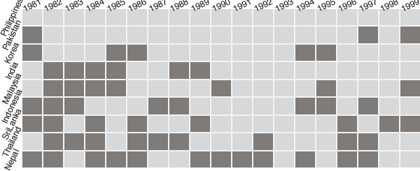
A plot of missing values on tariff rate information for nine Asian countries over 19 years. There is complete data for the Philippines and data for all countries in 1993. There are no striking patterns.
Reasons for missings and dealing with missings
Data can be missing for different reasons. It could be that a value was not recorded, or that it was, but was obviously an error and was consequently coded as missing. A value may be lost or incorrectly transcribed. In a survey people may not answer because they don’t know, because they don’t want to answer, because there is no option that matches their views, or because they were not asked. Or they may give a ridiculous answer, which the interviewer then marks as ‘missing’.
There is no standard missing code used by software (the NA used by R and other software is common). In the past, numbers like 99 or 999 were used and caused problems when people didn’t notice and calculated statistics and fitted models as if those were real numbers. The version of the Pima Indians dataset offered on the UCI Machine Learning Library uses 0 for entries the R version records as missings. Figure 9.5 shows a missing pattern plot for the Pima.tr2 dataset from MASS. Most of the records are complete. Quite a few cases are only missing a skin thickness value and a few values are missing on two of the other variables.
data(Pima.tr2, package="MASS")
visna(Pima.tr2, sort="b")
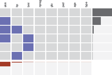
A missing value pattern plot for the Pima Indians dataset. Only three variables have missing values and no case is missing on all three.
The best that can be said is that all data (and documentation) should be looked at carefully before analysis. Other major statistics packages (SAS, SPSS, Stata) offer multiple missing codings to take account of different reasons for data being missing, but R does not; codings for more than one type of missing have to be sorted out by the user. As an example in practice, the US Multicenter Osteoarthritis Study (http://most.ucsf.edu/) has 13 different missing codes in its protocol.
Taking account of missing values can be important, especially if they are ‘not missing at random’ (NMAR). This is a term that became popular when multiple imputation was introduced [Rubin, 1987], the clever idea that instead of imputing a single value to substitute for a missing value, you should use several. NMAR data are distinguished from MCAR (Missing Completely At Random) and MAR (Missing At Random) (where missingness may depend on the value of the missing entry). One of the reasons the 1992 election in the UK was badly predicted was apparently that conservative voters were reluctant to admit to intending to vote conservative [Worcester, 1996], an example of MAR.
9.3 Outliers
What is an outlier?
Outliers are cases which are far away from the bulk of the data. They may be errors (a decimal point in the wrong place), genuine extreme values (some people are paid much more money than the rest of us), rare values (occasionally a lot of people are sick on the same day), unusual values (small people can be very heavy), cases of special interest (exceptional performances), or data from some other source (including a few small companies in a dataset on large companies). The last is sometimes referred to in the statistical literature as contamination.
Whether points are judged to be outliers depends on the data or model with which they are compared. A basketball player may be regarded as unusually tall amongst a group of his own age, whilst being average within a group of his fellow basketball players. Outliers are often talked about as if they are individual unusual values, but you often observe groups of outliers, particularly with large datasets, and one analyst’s outlying group may be another person’s population subset.
As groups of outliers get larger relative to the main part of a dataset, you could say you are looking for outliers or you are identifying distinct subsets or you are assessing how homogeneous the dataset is. This chapter concentrates on at most small groups of outliers and does not consider the more complex problem of dataset heterogeneity in large datasets. That is a topic for itself and depends particularly heavily on the context and aims of a study.
Possible outliers on individual variables are easy to spot graphically, and bivariate outliers, which are not outlying on the individual variables, can be seen in scatterplots. There can also be higher dimensional outliers that are not outliers on lower numbers of dimensions and these are trickier to find. That is hardly surprising: Try to think of what a three-dimensional outlier looks like which is neither a onedimensional outlier on any of its three dimensions nor a bivariate outlier on any of the three pairs of dimensions.
Determining outliers analytically is not easy. Many procedures have been suggested, but none are universally accepted, there are too many different kinds of outlier that might arise. Analytic approaches are useful for picking out extreme outliers (and every method should be able to manage that) and for providing a first filtering of the data to produce a set of possible outliers that can then be examined in more detail.
It is worth identifying outliers for a number of reasons. Bad errors should be corrected, genuine outlying values can be interesting in their own right, and many statistical methods may work poorly in the presence of outliers. Robust methods have been proposed for dealing with datasets with outliers. They are often computationally demanding.
There is a fairly extensive literature on outliers beginning with the classic text by Barnett and Lewis [Barnett and Lewis, 1994] and including more recently [Aggarwal, 2013].
Examples of outliers
Figure 9.6 shows a sample collection of plots for identifying potential outliers in a subset of the USCrimes dataset from the package TeachingDemos. You can see a boxplot of the murder rates in US States in 2010, a scatterplot of the rates of theft and vehicle theft, and a parallel coordinate plot of the rates for nine different crimes.

Plots of the crime rates by state in 2010 for the USCrimes dataset, used for identifying potential outliers.
The preparatory code for the plot involves some subsetting and restructuring. One important point to note is that the dataset USCrimes is a three-dimensional array, not a data frame, so it has to be converted to a table and a long data frame first. Then data for the year 2010 are chosen and the data for the US as a whole are excluded. Next the data frame is reformed with columns for each of the variables using the spread function from tidyr. Finally the rate variables are selected:
library(tidyr)
data(USCrimes, package="TeachingDemos")
names(dimnames(USCrimes)) <- c("State", "Year", "Crime")
US10 <- USCrimes %>% as.table %>%
as.data.frame(responseName = "Rate") %>%
filter(Year==2010 & State != "United States-Total") %>%
spread(Crime, Rate) %>% select(State, ends_with("Rate"))
The boxplot identifies two possible outliers and one is clearly hugely different from all the rest, the District of Columbia. This can be identified with
US10 %>% select(State, MurderRate) %>% filter(MurderRate > 10)
The scatterplot seems to show one extreme outlier on both theft rates, the District of Columbia again. Interestingly, a boxplot of TheftRate alone shows no outliers. The scatterplot also indicates two states looking like bivariate outliers. Neither California nor Nevada are extreme on the individual variables, but both have relatively higher vehicle theft rates compared to their theft rates. Finally the parallel coordinate plot, in which each axis has been scaled individually between 0 and 1, reveals that one state has extremely high values on six of the nine variables, obviously the District of Columbia and that another state has a particularly high rate of rape.
a <- ggplot(US10, aes("var", MurderRate)) +
geom_boxplot() + xlab("") +
ylab("Murder rate per 100,000 population")
b <- ggplot(US10, aes(TheftRate, VehicleTheftRate)) +
geom_point() +
xlab("Theft rate per 100,000 population") +
ylab("Vehicle theft rate per 100,000 population")
c <- ggparcoord(data = US10, columns = c(2:10),
scale="uniminmax") +
theme(axis.title.x =element_blank(),
axis.title.y =element_blank())
grid.arrange(arrangeGrob(a, b, ncol=2, widths=c(1, 4)),
c, nrow=2)
Univariate outliers
There have been many attempts to suggest rules and tests for determining whether points should be considered outliers and none of them are satisfactory in all situations. Using tests for assessing whether points are outliers is difficult, as the tests are primarily designed for testing individual points and you may want to test several.
The best-known approach for an initial look at the data is to use boxplots. Tukey suggested marking individual cases as outliers if they were more than 1.5 × IQR (the interquartile range) outside the hinges (basically the quartiles). Figure 1.8 showed boxplots for the six continuous variables in the Pima Indians dataset. There are no outliers on the first variable (plasma glucose concentration), both low and high outliers on blood pressure, and high outliers on the other four variables, with as many as nine for the diabetes pedigree function.
Figure 9.7 displays boxplots for the seven continuous variables from the diamonds dataset from package ggplot2, also used in Exercise 7 of Chapter 3. First the code selects the desired variables and then combines them all in a new long data frame, so that all plots can be drawn simultaneously with the last line. Note the use of the scales option to ensure individual scaling for each variable and the nrow option to put all plots in one row. The formatting options are necessary to clear the plots of irrelevant labelling.
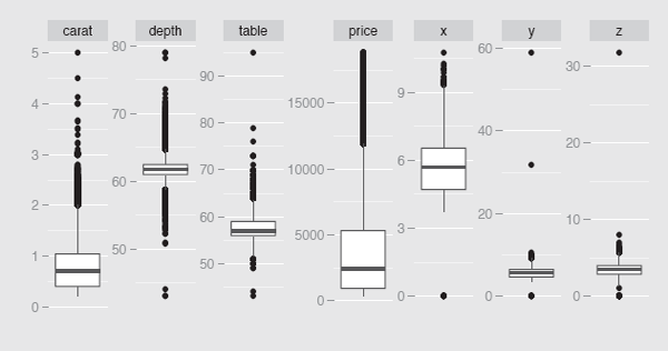
Individual boxplots of seven of the diamonds variables. Each of the variables has outliers, which is hardly surprising in a dataset of over 50 thousand cases. The last three variables, x, y, and z have cases with value 0, which must be wrong, and there are several high outliers, which must be wrong too. Both the carat and price variables are skewed to the right.
The differences in how Figure 1.8 and Figure 9.7 were drawn and what they show are worth noting. Traditional base graphics were used for Figure 1.8 and the boxplots for all the variables are shown in one display. This required that the variables were transformed to a common scale first. Graphics from ggplot2 were used for Figure 9.7. By pretending that all the variables were actually one long variable composed of different subsets it was possible to draw individual plots for each of them with a single command, using their actual scales.
Boxplots generally work well, although they tend to imply too many outliers for large datasets such as diamonds. The reason is clear: With large datasets there are sufficient numbers of points at intermediate outlying levels for them to be regarded as part of the population, even though boxplots plot them as outliers. At any rate, you can argue that it is better to identify too many potential outliers as too few. You are probably going to review the outliers in their order of ‘outlyingness’ anyway, and so the more extreme ones will be dealt with first.
Apart from obvious errors (e.g., digits have been transcribed, so that a temperature of 19° has been written as 91°), you need background knowledge to judge what kind of case an indicated outlier might be. In most applications there is information on many other variables and this can be used to help decide. Scatterplots can be used for looking at pairs of variables (as in Figure 9.8), while parallel coordinate plots are good for looking at more. Perhaps the case is an outlier on several variables, either in a consistent way (the District of Columbia in the USCrimes dataset in Figure 9.6) or in an inconsistent way (sometimes big, sometimes small). The latter may suggest a data shift error, where values have been entered in the wrong columns for a case.

Plots of y (width) and z (depth) from the diamonds dataset with and without 23 outliers and rescaled accordingly. Without the extreme outliers the plot is more informative and additional cases look suspicious.
When data have skew distributions, it is often a good idea to transform them, perhaps to a logarithmic scale. Points which were high outliers on the original scale
library(tidyr)
diam1 <- diamonds %>% select(carat, depth:z) %>%
gather(dX, dV, carat:z)
ggplot(diam1, aes("dX", dV)) + geom_boxplot() +
facet_wrap(~dX, scales = "free_y", nrow=1) +
xlab("") + ylab("") + scale_x_discrete(breaks=NULL)
will then no longer necessarily be outliers on the new scale and some points that were formerly regarded as non-outliers may now be low outliers. Again, background knowledge is essential to judge whether a transformation makes sense.
Multivariate outliers
Most outliers are outliers on at least one univariate dimension, sometimes several. The more variables there are, the more likely it is that cases are outliers on some dimension or other. This implies that the more variables you have, the more stringent the rules should be for deciding which cases might be outliers. In practice you usually start with the most extreme outliers and work inwards.
Multivariate measures depend on robust estimation of the parameters of the data. For small datasets the efficiency of calculating these robust statistics is good and there can only be a few outliers anyway. At least, you would think so. The famous stackloss dataset, a favourite amongst robust statisticians, has only 21 points and probably all of them have been declared an outlier at one time or another in some article or other [Dodge, 1996].
Large datasets are more complicated. It is much more likely that they are heterogeneous, the data quality is probably poorer, and there may well be a variety of outliers and outlying groups of diverse kinds. Whether this has much influence on an analysis is another matter. The diamonds dataset shows an example. The first plot in Figure 9.8 is a scatterplot of y and z (actually width and depth). There are some obvious errors (values of 0 and excessively high values). Restricting the ranges gives the second plot, which excludes 23 of the almost 54,000 points. Now some other cases appear to be in error (the three low values on depth), while others look unusual compared to the bulk of the data, bivariate outliers that are not outlying on either of width or depth alone.
a2 <- ggplot(diamonds, aes(y, z)) + geom_point() +
xlab("width") + ylab("depth")
d2 <- filter(diamonds, y > 2 & y < 11 & z > 1 & z < 7)
b2 <- ggplot(d2,aes(y, z)) + geom_point() +
xlab("width") + ylab("depth")
grid.arrange(a2, b2, ncol=2)
The statistics of the dataset including and excluding the original 23 outliers barely change, only the graphics are dramatically affected and that is because of the univariate outliers. Note how Hadley Wickham’s dplyr package is used for calculating the statistics.
diamS1 <- summarise(diamonds, meanx = mean(x), sdx = sd(x),
mean = mean(y), sdy = sd(y), corxy = cor(x,y))
diamS2 <- summarise(d2, meanx = mean(x), sdx = sd(x),
mean = mean(y), sdy = sd(y), corxy = cor(x,y))
diamS1
# meanx sdx meany sdy corxy
# 1 5.731157 1.121761 5.734526 1.142135 0.9747015
diamS2
# meanx sdx meany sdy corxy
# 1 5.731605 1.119402 5.733428 1.111272 0.9986573
Figure 9.8 also illustrates how points can be outliers on two dimensions without being outliers on the individual dimensions.
The decisions as to which points are outliers can be problematic and may depend on an implicitly assumed model. In Figure 9.9, showing the olive oil dataset used in two exercises in earlier chapters, you could regard points as outliers that are far from the mass of the data, or you could regard points as outliers that do not fit the smooth model well. Some points are outliers on both criteria.
data(olives, package="extracat")
ggplot(data=olives, aes(x=oleic, y=palmitic)) + geom_point>() +
geom_density2d(bins=4, col="red") + geom_smooth()

scatterplot of two of the variables from the olives dataset with contour lines from a two-dimensional density estimate and a loess smoother superimposed. Some points to the top left are outliers according to the density estimate, but not according to the smoother.
Higher dimensional outliers are tough to spot visually when they are not extremes on lower dimensions, and it is an open question how often such cases occur in real datasets. Suggested methods of finding them include using a robustified Mahalanobis distance and there have been several proposals how to do this in the literature [Ben-Gal, 2005]. Graphical displays such as parallel coordinate plots and scatterplot matrices can then be helpful for establishing why points have been identified as outliers.
A simple illustration is given in Figure 9.10, using the Boston dataset yet again, where the boxplot shows that there are low outliers on the variable ptratio, the pupil teacher ratio. Drawing a parallel coordinate plot of all the variables and colouring the three cases sharing the lowest value gives the plot on the right.
data(Boston, package="MASS")
a <- ggplot(Boston, aes("var", ptratio)) + geom_boxplot() +
xlab("") + ylab("Pupil-teacher ratio") +
scale_x_discrete(breaks=NULL)
Boston <- within(Boston, pt1 <- ifelse(ptratio < 13, 1, 0))
oc <- order(Boston$pt1)
b <- ggparcoord(data = Boston[oc,], columns = c(1:14),
scale="uniminmax", groupColumn="pt1") +
theme(axis.title.x = element_blank(),
axis.title.y = element_blank())
grid.arrange(a, b, nrow=1, widths=c(1,4))

A boxplot of ptratio from the Boston dataset and a parallel coordinate plot of all the variables with the three cases having the lowest value for ptratio coloured light blue. The three areas are very similar and are not outliers on any of the other variables.
Categorical variables divide datasets into subsets and often cases can be outliers within a subgroup but not on the whole dataset or the other way round. For a single subsetting variable, the best graphical approach is to plot boxplots for each of the categories. Figure 9.11 illustrates this for Sepal.Width in the iris dataset (cf. §1.3), where the boxplot for the three species together suggests four outliers, while
a <- ggplot(iris, aes("boxplot for all", Sepal.Width)) +
xlab("") + geom_boxplot() +
scale_x_discrete(breaks=NULL)
b <- ggplot(iris, aes(Species, Sepal.Width)) +
geom_boxplot() + xlab("")
grid.arrange(a, b, nrow=1, widths=c(1,2))

Boxplots of Sepal.Width for the iris dataset as a whole and for the three species separately. Four possible outliers are identified in each plot, while only one outlier is identified in both.
the boxplots for the three species separately also suggest four outliers, although only one of the points is an outlier in both displays.
Categorical outliers
It is easy enough to understand what is meant by an outlier on any continuous scale, but categorical outliers are rather different. The term could refer to cases which have some rare value on a categorical scale (e.g., purple hair), but that is more a matter of defining the categories appropriately for the analyses to be carried out.
The more interesting situation is where there are a number of categorical variables and certain combinations occur very infrequently or should not occur at all. In his study of data cleaning, [Malik, 2010], Waqas Ahmed Malik used a dataset from the Pakistani Labour Force Survey of 2003. He found a few cases of people who were divorced or widowed and who were classified on another variable as being the spouse of the head of household. Those cases were clearly in error on at least one of the variables. In another analysis he found people with low education and employment status recorded as being corporate managers. In a dataset with around 140,000 cases these kinds of issues are bound to arise. Fluctuation diagrams (cf. §7.4) are useful visual tools for finding such cases.
Dealing with outliers
Identifying cases as potential outliers, whether with graphical or with analytic methods, is relatively straightforward, what to do about the information is not. Outliers need to be inspected and reviewed. Sometimes they may be interesting in their own right (e.g., telephone companies have regarded unusual records as indicating fraud), sometimes they may be recognisable special cases (e.g., Bob Beamon’s long jump at the 1968 Olympic Games), and sometimes they may be just errors.
If the cases are obviously wrong, then those values may be discarded or, if possible, corrected. You can decide to discard whole cases or just the unacceptable values, and background knowledge is essential for these kinds of decisions. If only individual values are discarded, they may be treated as missing and substitute values may be imputed for them in one way or another. Imputation can be a tricky business and the appropriate expertise is called for. Whenever data are discarded, it is a sensible idea to record what has been done and why, to ensure that discussion of results is complete. When two people analyse the same data, but handle outliers in different ways, it can save a lot of time to have complete details of what has been done when you compare results.
Some statistics are little affected by outliers, medians for instance, but graphics are always affected, even by a single case, as default scales have to be drawn to incorporate all the data. (Of course, this only applies to outliers which are outlying on at least one dimension, cf. Figure 9.8. Solely high dimensional outliers do not affect scaling.) One extreme value in a million can reduce the rest of the dataset to a column in a histogram or to a heavily overdrawn point in a scatterplot. To see the structure of the main part of the dataset you have to zoom in, effectively ignoring the outliers. It would be helpful if graphics gave some clue when some points are excluded like this; you can easily forget about outliers that are not visible.
Keeping outliers and discarding them are the two alternative extremes. In modelling, robust methods attempt to reduce the effect of outliers by calculating a weighting for each case. Outliers that are far away may have little or no weight attached to them, whereas cases which are neither far away nor part of the main pattern of the data may be assigned a larger weight, although still lower than cases in the middle of the data. Each robust method will produce different weightings, and the choice of parameters within a method will also have an effect. The jury is still out on how best to proceed.
A possible strategy for outliers
‘Extreme’ outliers are likely to be errors or data from a quite different population and should be discarded or replaced with imputed values. ‘Ordinary’ outliers may be of some interest in their own right. Quite often they will affect statistical modelling less than one might fear, although it is as well to check what influence they have using a robust approach, if that is possible. Initially an exploration of the dataset with graphical methods and some simple outlier rules (e.g., a robust Mahalanobis distance) should suffice to get a feel for the data.
- Plot the onedimensional distributions. Examine any ‘extreme’ outliers to see if they are interesting in their own right, if they are obvious errors which can be corrected, or if they are values which should perhaps be discarded.
- For outliers which are ‘extreme’ on one dimension, examine their values on other dimensions. This can help to decide what to do about them. Consider imputing values for outlying values you intend to discard.
- After dealing with the ‘extreme’ values, examine further potential onedimensional outliers, i.e., those cases which are not ‘extreme’, but are marked as outliers by a boxplot or by some other rule. For these cases check the values on other dimensions using multivariate graphics, parallel coordinate plots, or sploms. Consider discarding cases which are outlying on more than one dimension.
- Cases which are outliers in higher dimensions, but not in lower ones, should be considered next. They may be identified in sploms (bivariate outliers), or in parallel coordinate plots, but it is probably best to use a robust multivariate approach and then inspect the possible outliers graphically to see why the analysis picked them out.
- Finally, consider whether outliers should be looked for in subsets of the complete dataset. Drawing boxplots by grouping variables is a good way of doing this. And, as always, any potential outliers found should be examined in conjunction with the case values on other variables and in the context of the study aims.
9.4 Modelling and testing for data quality
- Missing values
In principle some kind of binary pattern test could be carried out. In practice it is not done, probably because either there are not many missings or they have a readily interpretable pattern. - Univariate outliers
Many tests have been suggested and a helpful place to start is Barnett and Lewis [Barnett and Lewis, 1994]. Some unvariate tests are implemented in the package outliers. - Multivariate outliers
To use a criterion to identify a point as an outlier or to test for an outlier implies some kind of model of ‘standard’ data. No test is fully satisfactory, so much depends on the definition of ‘good’ data, on the possible numbers of outliers, and on the context. Different models and procedures will lead to different results. - Robust approaches
Modern approaches rely on robust estimation of the ‘good’ part of the data and, as with all robust methods, there is a wide range of possibilities involving clever heuristics of one kind or another. Robust Mahalanobis distances are key. Packages implementing the methods include robust base, mvoutlier, and CerioliOutlierDetection.
Main points
- Quality of data can be a major issue and there are many ways the quality of a dataset may be poor. All manner of different approaches may be helpful in identifying and solving the problems.
- Missing value pattern plots are good for identifying possible structure in missings (cf. Figure 9.2 and Figure 9.3).
- Outliers are difficult to define and pin down (§9.3). They may be compared to models or densities (Figure 9.9) or by subgroups (Figure 9.11).
- Individual extreme values are easy to spot, groups of outliers are more difficult to determine. There can be many different reasons for outliers, sometimes they are errors, sometimes they are important special cases.
- Graphical displays are useful for finding univariate outliers (Figure 9.7) and bivariate ones (Figure 9.8).
- Sploms and parallel coordinate plots can be helpful for studying potential outliers (Figure 9.10), for instance ones identified by robust approaches.
Exercises
- Lung cancer
The dataset lung in the package survival has 228 patients and 10 variables. What missing value patterns are there? - Academic Performance Index
The dataset apipop in the package survey comprises 6194 Californian schools. There are 37 variables in all.- (a) Are the missing values missing at random or are there patterns?
- (b) Does excluding the variables with a majority of missing values change the picture much?
- Diamonds
Discuss the various kinds of outlier identified in a scatterplot of the variables carat and width from the diamonds dataset discussed in Figure 9.7 and Figure 9.8. - Beamon’s longjump
The dataset MexLJ has the best longjumps by the 14 finalists in the 1968 Mexico Olympics. Is Bob Beamon’s famous jump really so very different from those of the other competitors? Draw an appropriate plot for investigating this. - Pearson heights
Pearsons’ height data for fathers and sons were considered in §3.3 and §5.4.- (a) Draw a scatterplot of the heights. Are there any cases you would regard as outliers?
- (b) Overlay your plot with a bivariate density estimate. Which cases do you think would be regarded as outliers under this model?
- Forbes2000
This dataset from the HSAUR2 package includes data for the sales, assets, profits, and market value for each of 2000 companies in 2004. Are there many univariate outliers? What about bivariate outliers? - Forbes2000 again
The three variables, sales, assets, and marketvalue, are all related to some extent to the size of the company. If they are transformed to logs, their distributions look far less skewed.- (a) How many cases are still possibly outliers?
- (b) Given that some companies reported losses, the variable profits can only be transformed to logs by excluding companies who failed to make profits. Which additional companies might then be considered to be outliers?
- Wheat
Rothamstead is the longest running agricultural research station in the world and is probably best known to statisticians because Fisher worked there from 1919 to 1933. In 1910 a study of wheat yields was carried out there and Figure 9.12 shows the grain and straw yields. Which of the points in the scatterplot might be outliers? Why? - USCrimes 2010
Create a subset of the USCrimes dataset in the TeachingDemos package containing just the data for 2010. As the District of Columbia is an extreme outlier on several of the rates, remove it from the dataset and carry out a graphical outlier analysis.- (a) How many univariate and bivariate outliers do you find?
- (b) Are they the same as the ones found in the dataset with the District of Columbia included?
- Boston housing
- (a) Compare a boxplot and a histogram of the tax variable. Which is more useful for investigating outliers and how many outliers are there?
- (b) Draw a parallel coordinate plot of all the variables and colour the cases with a high value for tax. Are these cases different from the rest on other variables?
- Intermission
The Mona Lisa by Leonardo da Vinci hangs in the Louvre museum in Paris. Is the Mona Lisa so different from other portraits of women?
