CHAPTER 12
Know Where You Really Make Money
“If a blind man leads a blind man, both will fall into a pit.”
—MATTHEW 15:13-14
Most companies do not truly know where or how they make money!
This may be a shocking statement, but upon reflection it should ring true. If your company is like many others, you know your overall costs, but you do not know your costs at a more granular and actionable level. You know how much overall profit you make, but you do not have a clear picture of your profitability by product or by customer. And like others, you probably have a strong belief that many things your company does, sells, or provides are in reality much more costly, and therefore less profitable, than your figures show.
And if this is the case, then the converse is also true—that some of what your company does is actually much less costly, and therefore much more profitable, than you may realize. We call these products, customers, segments, activities, and so on your islands of profit in your sea of costs.* But with all the cross-subsidizations that typically exist in most companies today, the picture for most is opaque at best, with the islands and sea blending together behind a fog bank.
Many executives have confided in us that they don’t truly believe the standard cost and profit figures their accounting or finance departments provide. They know that massive cross-subsidizations mask the true cost and profit of their products, customers, market segments, and activities. They have strong suspicions that particular products, customers, and regions are much more costly than the organization realizes. But the organization continues to manage its business, almost as a matter of faith, based on standard cost and profit figures, as it knows nothing else. The business is navigating choppier waters in an ever thickening fog bank.
This needn’t be the case. What would it mean if you could lift the fog and gain a clear view of your real cost and profit at the product, customer, and segment level? What would it mean if you really knew where you make, and lose, money?
In this chapter we discuss three steps toward navigating your profit trajectory:
1. Understanding where you make and lose money today (i.e., knowing your complexity-adjusted operating profit by product, customer, region, and so on)
2. Understanding how your profitability by product, customer, region, and so on can be expected to change if or as volume changes (i.e., knowing your profit scaling curves)
3. Understanding how greater or lesser levels of complexity can change your profit scaling curves (i.e., knowing how to shift your scaling curves)
What’s at Stake?
Navigation starts with knowing where you are, and growing in the Age of Complexity starts with knowing where you are making money and where you are not. Without a clearer and more granular view of real cost and profit than traditional costing methodologies and the vast majority of accounting and finance departments can provide, companies are as the blind leading the blind. Consider the implications:
![]() Undertaking product rationalization efforts without knowing how much profit each product actually generates
Undertaking product rationalization efforts without knowing how much profit each product actually generates
![]() Setting prices without knowing the real costs of your products and services
Setting prices without knowing the real costs of your products and services
![]() Advancing new products without understanding the likely full cost implications of those decisions, nor their impact on the profitability of other products
Advancing new products without understanding the likely full cost implications of those decisions, nor their impact on the profitability of other products
![]() Making decisions around resource investments without really knowing the likely full costs and therefore returns of those decisions—including underinvesting in the real drivers and creators of profit
Making decisions around resource investments without really knowing the likely full costs and therefore returns of those decisions—including underinvesting in the real drivers and creators of profit
![]() Making acquisitions based on synergies that not only are not achieved but were never really there for the taking
Making acquisitions based on synergies that not only are not achieved but were never really there for the taking
![]() Basing business plans on economies of scale that never materialize
Basing business plans on economies of scale that never materialize
Our premise here is this: in the Age of Complexity (1) most companies do not know, at an actionable level, where they really make money, and (2) without knowing where you make money you cannot reliably navigate to profitable growth.
Of course, once you know where you are—meaning where you make money—you must decide where to go. But unless you know this, nothing else matters. So this is where development of your navigation skills begin.
Beware Standard Cost and Profit
A theme in this book is that complexity has changed the game, rendering traditional approaches outmoded and more dangerous to rely upon. Chief among these is traditional product costing, commonly referred to as “standard cost.” (Next but not far behind is a common misplaced reliance on contribution margin, which we will get to later.)
Standard costs are full of cost allocations, but allocations based upon the outmoded fixed-variable cost paradigm of the Industrial Age—such as spreading overhead costs across a portfolio of products in proportion to each product’s sales. By not recognizing the impact of complexity costs, standard costing is left rife with cross-subsidizations. Further, as complexity has grown, the difference between standard cost/profit figures and the true cost/profit has only increased, and to untenable levels for many companies.
Borrowing some terms from Lean, all costs are either value-add (VA) or non-value-add (NVA). For example, the raw materials in a product are likely VA. So too is the time involved in the actual machining of a part—or perhaps the time to manufacture it at a gross production rate on a production line. But items such as setups or changeovers, indirect labor, losses and inefficiencies, the cost to transport, store, and handle inventory and WIP, and manufacturing overhead overall, not to mention corporate overhead, are by definition NVA. Standard costing tends to deal generally well with VA costs, which are more tangible and easier to measure and assign, but does not deal well with the ever increasing NVA costs, which are more difficult to assign to a specific product.*
Consider how we typically develop our standard cost figures: We may know the actual cost of something, such as we pay a supplier $2.65 per pound of copper, for example, and since Product A contains, say, two pounds of copper we put $5.30 toward the unit cost of Product A, and continue to other materials and other cost categories. This part is rather straightforward.
Increasingly, however, the costs that we put to a product are allocations of shared resources and costs—indirect costs and overheads—where the portion of the resource consumed by a specific product is much less clear or tangible than, say, the measurement of two pounds of copper. Although these costs are less tangible at a product or customer level, they are no less real, and without better methods for costing, and left with only the outmoded fixed-variable cost paradigm, we force ourselves to convert such costs into unit costs that are much easier to deal with. The result: we tend to “peanut butter” spread these costs, spreading them in proportion to volume (whether by revenue, units, weight, or so forth).
With no other approach, we treat all products as equal consumers of such overhead, other shared costs, and many inefficiencies, even though that is rarely the case. For example, we worked with a major brewer that for years had produced only a very small number of high-volume beers at its largest brewery. With essentially just two products, its namesake brand and the light version of the same, it was very easy to develop a production schedule. Then, with the growth of craft beers and the resulting growth in the number of the brewer’s products, and its packaging variety as well, the production schedule became a complex science at the brewery, necessitating creation of a production scheduling department. The cost of this department rolled up into manufacturing overhead, which was then allocated along with the rest of manufacturing overhead to individual products in proportion to their volume produced. The result was that the vast majority of the production scheduling cost was being borne by the two high-volume legacy products that had been relatively easy to schedule on their own, and not by the many lower-volume craft products that had necessitated creating the production scheduling department in the first place.
Granted, your standard costing may already account for some differences between your products and services in generating NVA costs. Perhaps you already account for one product requiring more setup time than another, or some products running slower or having higher scrap on your line, or some services being more time consuming to provide, but you likely don’t account for the fact that with all the variety of products, raw materials, WIP, and finished goods, your facility is larger and more sprawling, increasing travel time all around. You likely don’t account for the fact that some products (and costumers, segments, etc.) consume much more overhead, engineering, customer service and support, and other shared and overhead resources per unit than do other products.
However, it is likely that we don’t need to convince you that your standard cost figures increasingly don’t reflect reality. Based on our experience, we are confident that at some level you already believe this. Executives know this in their bones. In fact, for years many intrepid executives have tried to tackle this issue, attempting to sort through this complex costing mess, almost to the point that they have given up. But don’t give up just yet.
ABC Falls Short
Activity-based costing (ABC) was to be the panacea for our costing ills. Developing in the 1970s and 1980s in the manufacturing sector, and defined in 1987 by Robert Kaplan and William Bruns in their book Accounting and Management: A Field Study Perspective, ABC initially sought to account for the indirect and overhead costs left out of traditional cost accounting, and later to correct for the growing cross-subsidizations involved in standard costing to more correctly allocate indirect costs to specific products.
However, ABC grew too cumbersome. While well intentioned and in several applications even useful, ABC was not able to keep pace with the growing complexity of our world. In application, ABC began to fail under its own weight, falling prey to the complexity it was meant to address.
We consider ABC a “bottom-up” approach. It involves identifying all indirect activities and assigning the cost of each activity to all products (or customers) based on the actual consumption by each. This worked well when the level of complexity—the variety of activities and products—was, although material, still low. It worked as a method of complexity costing when the level of complexity was still not that high. It was a temporary solution. With greater complexity there became ever more and smaller-volume activities to identify, and many more products to assign cost to. As complexity grew, the level of effort required to apply ABC grew exponentially, and ABC initiatives became enormous, cumbersome, and resource intensive projects that strained under their own weight.
Further, ABC is a very static exercise, yet the more complex a system is the more dynamic it tends to be. After counting all the “beans” and assigning costs to all products and/or services, and adding everything up, the resulting answer only reflects the organization as it was when it was counted. Once processes or the product/service portfolio is changed—often in response to the results of the ABC study—one would have to count all over again to see the new cost picture. And in a complex system, things are highly intertwined—impacting one area tends to affect a myriad of other areas.
However informative, such efforts in today’s complex world become so unwieldly and impractical that executives often simply abandon them or never want to repeat them. Indeed, we have met many a battle-scared senior executive that never wants to go through an ABC effort again.
But ABC’s being an impracticable solution for today’s costing crisis does not mean that the need for and value from knowing where you really make money has abated. Rather, it is as important as ever. We just needed different tools.
Square Root Costing
Square Root Costing (SRC) is the most exciting development in the world of costing in many years. It is a practical methodology for correcting the cross-subsidizations that have plagued standard costing, and is far faster, much less cumbersome, and significantly less resource intensive than ABC. SRC can accomplish this because it is the only costing methodology based on an accurate understanding of complexity costs. It isn’t constrained to the outmoded fixed-variable cost paradigm. It recognizes complexity costs as a category of costs on their own with their own unique dynamics, rather than force-fitting them into buckets as either variable costs or fixed costs, neither of which they are. In short, it is a costing methodology suited for today’s complex world.
SRC is easier and faster since it is not a bottom-up “count the beans” approach like ABC. Rather, it is a top-down, allocation-driven costing approach, as is standard costing, but importantly with a broader menu of allocations methods than standard costing.
Many of our clients, using SRC, have quickly gained a much clearer view of their true product and customer profitability, blowing away the fog obscuring their islands of profit and exposing a sea of costs. These companies have used SRC to inform product and service portfolio optimization efforts and product strategies; develop new product costing models and business rules for product management, including minimum efficient volumes for products, product families, brands, regions, and so on; and broadly, to inform strategic decisions.
Invariably, they find that their small-volume products, services, customers, regions, and activities are more costly and less profitable than reflected in their standard cost, often much more so. This does not necessarily mean that these products and services are unprofitable, as the price point may be sufficiently high to cover the costs, but they are almost always not as profitable as they had appeared.
The reason is simple: complexity is the opposite of scale. Remember, as we described in Chapter 3, complexity breaks up scale, and profitability is driven more by economies of density (revenue divided by complexity) than economies of scale (simply revenue). Larger-volume products deliver relatively more scale, and relatively less complexity (i.e., are more dense); whereas smaller-volume products deliver relatively more complexity, for relatively less scale (i.e., are less dense).
Figure 12.1 shows complexity-adjusted operating margins by product segment for one of our clients, a major beverage company. Product Segment C includes the company’s major legacy brands. While it still comprised the majority of the company’s sales volume, overall sales in this market segment were flat and price points had been slowly declining, which had created pressure to find new and growing market segments.
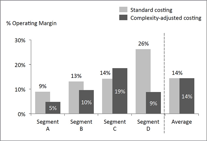
FIGURE 12.1: Complexity-Adjusted Operating Margin vs. Standard Operating Margin for a Major Beverage Company
Segment D represented a new and growing market opportunity, which consisted of specialty products with much higher price points; hence this was where the excitement, and investment, was. Understandably, the company’s standard cost figures showed operating margins in Segment D, at 26 percent, to be much higher than that of Segment C, at just 14 percent.1 With its specialty products and much higher price point, it seemed to reason that the exciting new specialty segment (D) should be more profitable than the old, staid legacy (C).
But these standard cost figures did not account for all the complexity and associated costs that were incurred in order to aggressively compete in and develop and deliver the specialty products making up Segment D. Adjusting for the real costs of this complexity showed not just that the legacy segment was subsidizing the specialty segment, but that the legacy segment was still the most profitable, at 19 percent operating margin, versus the specialty segment’s much more accurate figure of 9 percent operating margin.2 The cost of all of the unrestrained product proliferation incurred in going after the specialty more than consumed the potential value afforded by the high price points.
However, given the flat to declining legacy segment, and higher price point and growth in the specialty segment, the answer was not to shift away from Segment D, but rather to pursue that segment in a more methodical, disciplined, and purposeful manner, moving away from a “throw it at the wall and see what sticks” approach to product development to a more disciplined product management approach with business rules for minimum effective density, specific targets for product volumes, and culling of unsuccessful products.
Looking Under the Hood of SRC
How does SRC work? SRC is a top-down allocation methodology based on a fuller understanding of cost in today’s complex world. In Chapter 2 we introduced the three types of cost: variable costs, fixed costs, and complexity costs. These costs vary proportionally with volume, are independent of volume, or grow exponentially with complexity, respectively; and each of these costs dominated the Preindustrial Age, the Industrial Age, and the Age of Complexity, respectively. It is important to understand the dynamics behind each of these costs, so first a little review:
![]() Variable costs. Traditional variable costs are simply proportional to some measure of volume (whether tons, gallons, dollars, hours, etc.). If you double the volume, from say two pounds of copper to four, you double the cost. This relationship is shown as a straight line in Figure 12.2a1, where the unit cost (for example, $2.65 per pound of copper) determines the slope of the line. The unit cost is independent of volume, meaning that it doesn’t change over the range of volumes. Therefore, the unit cost is constant, as shown in Figure 12.2a2.
Variable costs. Traditional variable costs are simply proportional to some measure of volume (whether tons, gallons, dollars, hours, etc.). If you double the volume, from say two pounds of copper to four, you double the cost. This relationship is shown as a straight line in Figure 12.2a1, where the unit cost (for example, $2.65 per pound of copper) determines the slope of the line. The unit cost is independent of volume, meaning that it doesn’t change over the range of volumes. Therefore, the unit cost is constant, as shown in Figure 12.2a2.
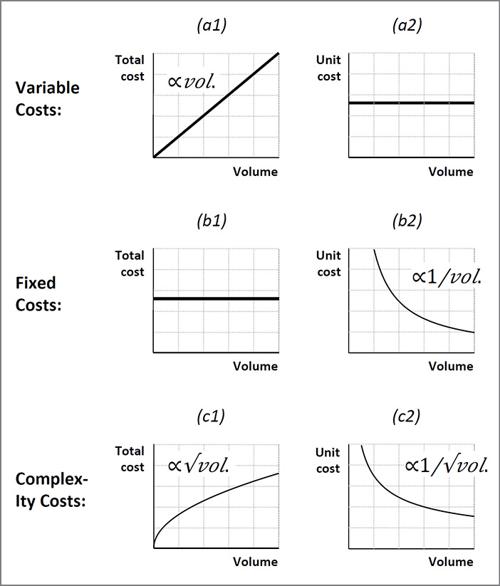
FIGURE 12.2: Relationship of Cost with Volume, for Variable, Fixed, and Complexity Costs
![]() Fixed costs. Fixed costs are almost the opposite of variable costs. With fixed costs, it is the total cost, and not the unit cost, that is constant over volume (see Figure 12.2b1). Another way to say this is that cost is independent of volume. For example, most design, engineering, product development, and registration costs for a product are independent of the volume sold of the product. Some quality costs also fall into this category. For example, if one must perform a quality check on an ingredient tank each day, regardless of how much of the ingredient is added or used from the tank, then the cost of that quality check is independent of the volume of the ingredient used. Importantly, if the total cost is independent of volume, then the cost per unit is highly dependent on volume, and drops rapidly as the fixed cost is spread over more units (see Figure 12.2b2).
Fixed costs. Fixed costs are almost the opposite of variable costs. With fixed costs, it is the total cost, and not the unit cost, that is constant over volume (see Figure 12.2b1). Another way to say this is that cost is independent of volume. For example, most design, engineering, product development, and registration costs for a product are independent of the volume sold of the product. Some quality costs also fall into this category. For example, if one must perform a quality check on an ingredient tank each day, regardless of how much of the ingredient is added or used from the tank, then the cost of that quality check is independent of the volume of the ingredient used. Importantly, if the total cost is independent of volume, then the cost per unit is highly dependent on volume, and drops rapidly as the fixed cost is spread over more units (see Figure 12.2b2).
These descriptions capture the essence of standard costing. When allocating costs, we treat costs as either fixed or variable, and since fixed is rather extreme, when in doubt we usually allocate costs as variable costs, meaning we peanut butter spread those costs in such a way that we treat all products, customers, and so on as equal generators of those costs, masking real differences between products (and customers, etc.) in generating those costs and creating cross-subsidizations in the process.
However, a significant and growing portion of costs—the large majority of NVA and complexity costs—fit neither variable nor fixed cost categories. These costs tend to go up with volume, but not proportionally with it.3 Also, their cost per unit tends to drop with volume, but not as steeply as that of truly fixed costs. In our work and research we have discovered and categorized this third category of cost:
![]() Complexity costs. Complexity costs tend to follow a square root of volume relationship, meaning that the cost is proportional to the square root of the volume; and since unit cost is simply cost divided by volume, the cost per unit is proportional to the inverse square-root of the volume (see Figures 12.2c1 and 12.2c2).4
Complexity costs. Complexity costs tend to follow a square root of volume relationship, meaning that the cost is proportional to the square root of the volume; and since unit cost is simply cost divided by volume, the cost per unit is proportional to the inverse square-root of the volume (see Figures 12.2c1 and 12.2c2).4
This is a very powerful relationship to understand and take into account in costing. Mathematically, it may look as if complexity costs are just in between the other two methods, so perhaps even without it things would “average out” and come to a good enough answer. However, in practice, this is anything but the case. For costs above gross margin, we tend to mistreat complexity costs as variable costs, yet below gross margin we tend to treat complexity costs as fixed costs. This has two insidious and compounding effects.
First, for costs above the gross margin line—essentially cost of goods sold (COGS)—we tend to mistreat complexity costs as variable costs, peanut butter spreading these costs, with the result that we “undercost” small-volume, less-dense products, customers, activities, and so on. By undercosting small-volume things, we undercost complexity, making complexity appear less costly in our figures, and therefore making organizations more tolerable of taking on more complexity. We pointed out in our first book that the costs of complexity are often hidden, which is in part due to treating complexity costs as traditional variable costs. But while these costs may be hidden, they are still very real. By taking on more complexity, we take on more hidden costs, which we subsidize from our islands of profit, making those islands appear a bit smaller and less profitable than they truly are.
Second, below gross margin—essentially SG&A—we tend to mistreat complexity costs as fixed costs, suggesting that as we add more complexity and revenue, those fixed costs will not grow. But we know from experience that this so often fails to be the case. By mistreating complexity costs below gross margin as fixed costs, we overestimate our potential for fixed-cost leverage, meaning we overestimate the promise of economies of scale (we have seen many a business plan based on economies of scale that the business never realized). By overestimating the promise of economies of scale, your organization is more willing to take on complexity—since it doesn’t anticipate the complexity costs that come along with it.
In both cases, by mistreating complexity costs as either variable costs or fixed costs, you will underestimate the cost of complexity; and by underestimating its cost, you leave yourself more tolerable and accepting of taking on more complexity, adding hidden costs, obscuring your islands of profit, and eroding the very economies of scale you may be expecting to realize.
By correctly treating complexity costs, SRC presents a clear picture—showing the costs as they truly are, removing the fog bank obscuring your islands of profit and sea of costs, and presents a realistic view of your potential to leverage your real fixed costs and gain scale economies. It is to this last point we turn next, as once you know where you are, you must decide where to go. As you grow your business, how will your costs and profit grow? Will they grow at the same pace, leaving you larger but no more profitable than you are today, or like half of all companies will your costs grow faster than your profits, leaving you larger but less profitable than you are today?
Minimum Efficient Volume?
Managing complexity often comes down to establishing business rules informed by the cost of complexity.
Standard costing tends to undercost small-volume products—leaving larger products (or customers, regions, etc.) to subsidize smaller ones. In correcting for this, SRC tends to shift costs to smaller-volume products. This begs the question, how much more costly are small-volume products than large-volume products, and what is the minimum efficient scale for a product, product family, brand, and so on?
Of course this depends on your particular company, industry, and product portfolio. Figure 12.3 shows a comparison between the complexity-adjusted conversion cost and standard conversion costs by product for an industrial manufacturing company. In this case, small-volume products were as much as six times more costly to produce than their standard cost figures had shown. Also, below annual volume of 10,000 units, the unit price began to rise dramatically. This suggests a minimum efficient volume of 10,000 units per year. Of course, this doesn’t mean that products with less than this amount should be eliminated, but does mean that those products have not, or haven’t yet, reached an efficient volume threshold.
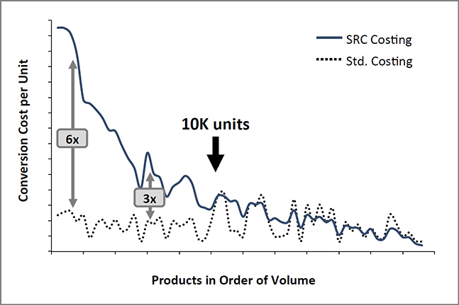
FIGURE 12.3: Comparison of SRC and Standard Costing Conversion Costs per Unit by Product for an Industrial Manufacturer
Return of Scaling Curves
Scaling curves simply show how some measure, for example a company’s cost or profit, can be expected to change as revenue grows. A cost scaling curve shows how costs will grow with volume. A profit scaling curve shows how your profit or profitability will change with volume. In the Industrial Age scaling curves were straightforward though important. For example, if a company had $2 million in revenue, and $2 million in costs, half of which were variable and the other half fixed, it would have zero profit. But if it could double its revenue to $4 million (assuming pricing remained the same), it would also double its variable costs to $2 million, yet its fixed costs would remain $1 million, yielding $1 million in profit. The company’s profitability would grow from zero percent of $2 million in revenue to 25 percent of $4 million in revenue. Economies of scale indeed.
Although it is much more complex today, companies still need to manage their scaling curves. But despite the need, most companies do not have a clear view at all on how their costs and profit are set to change with scale—and those that believe they do are often disappointed when expected economies of scale fail to materialize. Traditional costing methods are unable to provide scaling curves for several reasons: the errors inherent in standard cost and standard profit figures would be exacerbated and make scaling curves derived from such figures even more unreliable; standard cost approaches typically don’t include SG&A, which must be a key part of any meaningful cost curves for managing corporate profit trajectory; and ABC is too cumbersome and not set up for translating its results to a range of volumes. However, because SRC is still an allocation methodology, it is very easy to develop scaling curves—much as it was very easy to develop scaling curves from standard cost figures in the Industrial Age.5
Figure 12.4 shows such scaling curves for a variety of products offered by an industrial supply company. All of these products (A through G) had showed positive operating margin based on standard costing. However SRC showed that only two of them (products A and C) were actually operating margin positive. But the scaling curves revealed much more. They showed products B and D to be subscale, meaning that with sufficient growth they could become operating margin positive, to more than 30 percent and 20 percent, respectively. Product E, with enough growth, would only become marginally profitable. Scaling curves also show how much sales for an unprofitable product (or product family, product line, brand, or customer) would have to increase to become profitable.
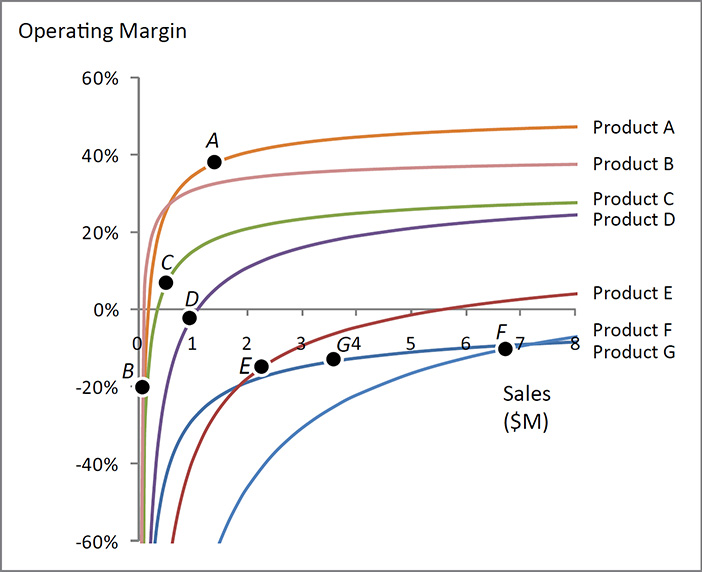
FIGURE 12.4: Profit Scaling Curves
On the other hand, products G and F were intrinsically unprofitable, meaning that they would remain unprofitable at any reasonable volume. Whereas the company explored opportunities to grow products B, D, and E, the answer for products F and G was to look for opportunities to transform or eliminate these products.
Profit scaling curves can be drawn for any revenue-producing item or groups of items. They can be drawn for products, product families, product categories, market segments, customers, countries, and regions. Clearly, understanding your profit scaling across these many dimensions adds tremendous clarity as you chart a course for profitable growth. The next step is to understand how complexity—adding or removing complexity—changes the shapes of these curves.
Shifting the Curve
If we were to consolidate several products into one product, retaining the same total revenue, we would reduce complexity for the same revenue, and increase density. By reducing complexity, we would gain economies of density, increasing the profitability of the associated revenue.
Removing complexity—for example, pruning a product line—shifts the associated profit scaling curve upward. Conversely, adding complexity shifts the associated profit scaling curve downward (see Figure 12.5). Often, we are adding products—i.e., complexity—to increase sales and revenue. We see ourselves marching along and upward on the profit scaling curve, expecting to enjoy not just more revenue but also greater profitability. But as we add complexity, the curve sinks, and as this cycle continues we find ourselves running up a sinking curve. If we can run up the curve faster than it sinks, then we will increase profitability. On the other hand, if we sink the curve faster than we run up it, we will reduce profitability. This leads us back to our earlier rule of thumb—introduced in Chapter 3—that if we add revenue faster than complexity, we will tend to become more profitable; whereas if we add complexity faster than revenue we will tend to become less profitable.
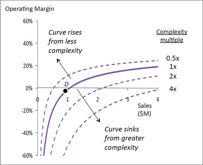
FIGURE 12.5: Shifting the Profit Scaling Curve
The real opportunity lies in marching up a rising curve; in decreasing overall complexity while increasing revenue, with dramatic increase in density and profitability. How do we do this? This takes us to our next chapter.
* Referring back to the Whale Curve introduced in Chapter 2 and covered in more depth in our first book, Waging War on Complexity Cost, the islands of profit are the 20 to 30 percent of products that in many companies generate over 300 percent of profits; and the sea of costs are the remaining 70 to 80 percent of products that destroy 200 percent or more of profits.
* Remember, complexity costs tend to grow exponentially with the level of complexity. And while complexity costs and NVA costs are not necessarily the same, complexity is what drives NVA costs to be so large. At a practical level, where NVA costs are large, we can then treat them as complexity costs. For more information on how complexity drives NVA costs, see our first book, Waging War on Complexity Costs.