
Skills, Tasks and Technologies: Implications for Employment and Earnings*
Daron Acemoglu, * MIT, NBER and CIFAR
David Autor, ** MIT, NBER and IZA
Abstract
A central organizing framework of the voluminous recent literature studying changes in the returns to skills and the evolution of earnings inequality is what we refer to as the canonical model, which elegantly and powerfully operationalizes the supply and demand for skills by assuming two distinct skill groups that perform two different and imperfectly substitutable tasks or produce two imperfectly substitutable goods. Technology is assumed to take a factor-augmenting form, which, by complementing either high or low skill workers, can generate skill biased demand shifts. In this paper, we argue that despite its notable successes, the canonical model is largely silent on a number of central empirical developments of the last three decades, including: (1) significant declines in real wages of low skill workers, particularly low skill males; (2) non-monotone changes in wages at different parts of the earnings distribution during different decades; (3) broad-based increases in employment in high skill and low skill occupations relative to middle skilled occupations (i.e., job “polarization’’); (4) rapid diffusion of new technologies that directly substitute capital for labor in tasks previously performed by moderately skilled workers; and (5) expanding offshoring in opportunities, enabled by technology, which allow foreign labor to substitute for domestic workers specific tasks. Motivated by these patterns, we argue that it is valuable to consider a richer framework for analyzing how recent changes in the earnings and employment distribution in the United States and other advanced economies are shaped by the interactions among worker skills, job tasks, evolving technologies, and shifting trading opportunities. We propose a tractable task-based model in which the assignment of skills to tasks is endogenous and technical change may involve the substitution of machines for certain tasks previously performed by labor. We further consider how the evolution of technology in this task-based setting may be endogenized. We show how such a framework can be used to interpret several central recent trends, and we also suggest further directions for empirical exploration.
Keywords
College premium; Directed technical change; Earnings inequality; Occupations; Returns to schooling; Skill biased technical change; Skill premium; Tasks; Wage inequality
JEL classification: J20; J23; J24; J30; J31; O31; O33
1. Introduction
The changes in the distribution of earnings and the returns to college over the last several decades in the US labor market have motivated a large literature investigating the relationship between technical change and wages. The starting point of this literature is the observation that the return to skills, for example as measured by the relative wages of college graduate workers to high school graduates, has shown a tendency to increase over multiple decades despite the large secular increase in the relative supply of college educated workers. This suggests that concurrent with the increase in the supply of skills, there has been an increase in the (relative) demand for skills. Following Tinbergen’s pioneering (1974; 1975) work, the relative demand for skills is then linked to technology, and in particular to the skill bias of technical change. This perspective emphasizes that the return to skills (and to college) is determined by a race between the increase in the supply of skills in the labor market and technical change, which is assumed to be skill biased, in the sense that improvements in technology naturally increase the demand for more “skilled” workers, among them, college graduates (relative to non-college workers).
These ideas are elegantly and powerfully operationalized by what we refer to as the canonical model, which includes two skill groups performing two distinct and imperfectly substitutable occupations (or producing two imperfectly substitutable goods).1 Technology is assumed to take a factor-augmenting form, and thus complements either high or low skill workers. Changes in this factor-augmenting technology then capture skill biased technical change.2 The canonical model is not only tractable and conceptually attractive, but it has also proved to be empirically quite successful. Katz and Murphy (1992), Autor et al. (1998, 2008), and Carneiro and Lee (2009), among others, show that it successfully accounts for several salient changes in the distribution of earnings in the United States. Katz et al. (1995), Davis (1992), Murphy et al. (1998), Card and Lemieux (2001a), Fitzenberger and Kohn (2006) and Atkinson (2008) among others, show that the model also does a good job of capturing major cross-country differences among advanced nations. Goldin and Katz (2008) show that the model, with some minor modifications, provides a good account of the changes in the returns to schooling and the demand for skills throughout the entire twentieth century in the United States.
In this paper, we argue that despite the canonical model’s conceptual virtues and substantial empirical applicability, a satisfactory analysis of modern labor markets and recent empirical trends necessitates a richer framework. We emphasize two shortcomings of the canonical model. First, the canonical model is made tractable in part because it does not include a meaningful role for “tasks,” or equivalently, it imposes a one-to-one mapping between skills and tasks. A task is a unit of work activity that produces output (goods and services). In contrast, a skill is a worker’s endowment of capabilities for performing various tasks. Workers apply their skill endowments to tasks in exchange for wages, and skills applied to tasks produce output. The distinction between skills and tasks becomes particularly relevant when workers of a given skill level can perform a variety of tasks and change the set of tasks that they perform in response to changes in labor market conditions and technology. We argue that a systematic understanding of recent labor market trends, and more generally of the impact of technology on employment and earnings, requires a framework that factors in such changes in the allocation of skills to tasks. In particular, we suggest, following Autor et al. (2003), that recent technological developments have enabled information and communication technologies to either directly perform or permit the offshoring of a subset of the core job tasks previously performed by middle skill workers, thus causing a substantial change in the returns to certain types of skills and a measurable shift in the assignment of skills to tasks.
Second, the canonical model treats technology as exogenous and typically assumes that technical change is, by its nature, skill biased. The evidence, however, suggests that the extent of skill bias of technical change has varied over time and across countries. Autor et al. (1998), for example, suggest that there was an acceleration in skill bias in the 1980s and 1990s.3 Goldin and Katz (2008) present evidence that manufacturing technologies were skill complementary in the early twentieth century, but may have been skill substituting prior to that time. The available evidence suggests that in the nineteenth century, technical change often replaced—rather than complemented—skilled artisans. The artisan shop was replaced by the factory and later by interchangeable parts and the assembly line, and products previously manufactured by skilled artisans started to be produced in factories by workers with relatively few skills (e.g., Hounshell, 1985; James and Skinner, 1985; Mokyr, 1992; Goldin and Katz, 2008). Acemoglu (1998, 2002a) suggested that the endogenous response of technology to labor market conditions may account for several such patterns and significantly enriches the canonical model.
To build the case for a richer model of skill demands and wage determination, we first provide an overview of key labor market developments in the United States over the last five decades, and in less detail, across European Union economies. This overview enables us to highlight both why the canonical model provides an excellent starting point for any analysis of the returns to skills, and also why it falls short of providing an entirely satisfactory framework for understanding several noteworthy patterns. In particular, in addition to the well-known evolution of the college premium and the overall earnings inequality in the United States, we show that (1) low skill (particularly low skill male) workers have experienced significant real earnings declines over the last four decades; (2) there have been notably non-monotone changes in earnings levels across the earnings distribution over the last two decades (sometimes referred to as wage “polarization”), even as the overall “return to skill” as measured by the college/high school earnings gap has monotonically increased; (3) these changes in wage levels and the distribution of wages have been accompanied by systematic, non-monotone shifts in the composition of employment across occupations, with rapid simultaneous growth of both high education, high wage occupations and low education, low wage occupations in the United States and the European Union; (4) this “polarization” of employment does not merely reflect a change in the composition of skills available in the labor market but also a change in the allocation of skill groups across occupations—and, in fact, the explanatory power of occupation in accounting for wage differences across workers has significantly increased over time; (5) recent technological developments and recent trends in offshoring and outsourcing appear to have directly replaced workers in certain occupations and tasks. We next provide a briefoverview of the canonical model, demonstrate its empirical success in accounting for several major features of the evolving wage distribution, and highlight the key labor market developments about which the canonical model is either silent or at odds with the data.
Having argued that the canonical model is insufficiently nuanced to account for the rich relationships among skills, tasks and technologies that are the focus of this chapter, we then propose a task-based framework for analyzing the allocation of skills to tasks and for studying the effect of new technologies on the labor market and their impact on the distribution of earnings. We further show how technology can be endogenized in this framework.4
The framework we propose consists of a continuum of tasks, which together produce a unique final good. We assume that there are three types of skills—low, medium and high—and each worker is endowed with one of these types of skills.5 Workers have different comparative advantages, a feature that makes our model similar to Ricardian trade models. Given the prices of (the services of) different tasks and the wages for different types of skills in the market, firms (equivalently, workers) choose the optimal allocation of skills to tasks. Technical change in this framework can change both the productivity of different types of workers in all tasks (in a manner parallel to factor-augmenting technical change in the canonical model) and also in specific tasks (thus changing their comparative advantage). Importantly, the model allows for new technologies that may directly replace workers in certain tasks. More generally, it treats skills (embodied in labor), technologies (embodied in capital), and trade or offshoring as offering competing inputs for accomplishing various tasks. Thus, which input (labor, capital, or foreign inputs supplied via trade) is applied in equilibrium to accomplish which tasks depends in a rich but intuitive manner on cost and comparative advantage.
We show that even though this framework allows for an endogenous allocation of skills to tasks and a richer interaction between technology and wages than the canonical model, it is tractable. Relative wages of high to medium and medium to low skill workers are determined by relative supplies and task allocations. The canonical model is in fact a special case of this more general task-based model, and hence the model generates similar responses to changes in relative supplies and factor-augmenting technical change. Nevertheless, there are also richer implications because of the endogenously changing allocation of skills to tasks. Notably, while factor-augmenting technical progress always increases all wages in the canonical model, it can reduce the wages of certain groups in this more general model. Moreover, other forms of technical change, in particular the introduction of new technologies replacing workers in certain tasks, have richer but still intuitive effects on the earnings distribution and employment patterns.
We then show how this framework can be enriched by endogenizing the supply of skills and technology. We finally show how the mechanisms proposed by this framework suggest new ways of analyzing the data and provide some preliminary empirical evidence motivated by this approach.
The rest of the paper is organized as follows. The next section, Section 2, provides an overview of labor market trends, with an emphasis on changes in the earnings distribution, in the real wages of different demographic groups, in the distribution of employment by occupation, and in the allocation of skill groups to job tasks. Section 3 provides a briefrecap of the canonical model, which has become the natural starting point of most analyses of recent labor market trends, and explains why several of the patterns highlighted in Section 2 are challenging for the canonical model and suggest the need to move beyond this framework. Section 4 presents a tractable task-based model of the labor market, which we then use to reinterpret the patterns discussed in Section 2. Section 5 provides a first look at the evolution of real wages by demographic groups in the US labor market through the lens of the framework developed in Section 4. Section 6 concludes with a brief summary and with several areas for future research suggested by our paper. Two appendices contain additional details on the sources and the construction of the data used in the text and some further theoretical arguments.
2. An overview of labor market trends
This section provides an overview of trends in education, wage levels, wage distribution, and occupational composition in the US labor market over the last five decades, and also offers some comparisons with labor market developments in European Union economies. Our objective is not to provide a comprehensive account of labor market developments but to highlight those that we view as most relevant for understanding the changing structure of the supply and demand for skills.6 We focus on changes in earnings levels and earnings inequality not only because of the intrinsic importance of the topic but also because the evolution of the wage distribution provides information on how the market values of different types of skills have changed over time.
2.1. A brief overview of data sources
To summarize the basic changes in the US wage structure over the last five decades, we draw on four large and representative household data sources: the March Current Population Survey (March CPS), the combined Current Population Survey May and Outgoing Rotation Group samples (May/ORG CPS), the Census of Populations (Census), and the American Community Survey (ACS).7 We describe these sources briefly here and provide additional details on the construction of samples in the Data Appendix. The March Annual Demographic Files of the Current Population Survey offer the longest high-frequency data series enumerating labor force participation and earnings in the US economy. These data provide reasonably comparable measures of the prior year’s annual earnings, weeks worked, and hours worked per week for more than four decades. We use the March files from 1964 to 2009 (covering earnings from 1963 to 2008) to form a sample of real weekly earnings for workers aged 16 to 64 who participate in the labor force on a full-time, full-year (FTFY) basis, defined as working 35-plus hours per week and 40-plus weeks per year.
We complement the March FTFY series with data on hourly wages of all current labor force participants using May CPS samples for 1973 through 1978 and CPS Outgoing Rotation Group samples for 1979 through 2009 (CPS May/ORG). From these sources, we construct hourly wage data for all wage and salary workers employed during the CPS sample survey reference week. Unlike the retrospective annual earnings data in the March CPS, the May/ORG data provide point-in-time measures of usual hourly or weekly earnings. We use CPS sampling weights for all calculations.8
As detailed in Autor et al. (2005) and Lemieux (2006b), both the March and May/ORG CPS surveys have limitations that reduce their consistency over the fifty year period studied. The March CPS data are not ideal for analyzing the hourly wage distribution since they lack a point-in-time wage measure and thus hourly wages must be computed by dividing annual earnings by the product of weeks worked last year and usual weekly hours last year. Estimates of hours worked last year from the March CPS appear to be noisy, and moreover, data on usual weekly hours last year are not available prior to the 1976 March CPS. The May/ORG samples provide more accurate measures of the hourly wage distribution (particularly for hourly workers) but cover a shorter time period than the March CPS. Both the March and May/ORG CPS samples have undergone various changes in processing procedures over several decades that affect the top-coding of high earnings, the flagging of earning imputations, and the algorithms used for allocating earnings to individuals who do not answer earnings questions in the survey. These changes create challenges in producing consistent data series over time, and we have tried to account for them to the greatest extent possible.9
To analyze levels and changes in occupational structure within and across detailed demographic groups, we exploit the 1960, 1970, 1980, 1990 and 2000 Census of Populations and the 2008 American Community Survey (ACS). Because these data sources provide substantially larger samples than either the March or May/ORG surveys, they are better suited for a fine-grained analysis of changing occupational employment patterns within detailed demographic groups.10 The earnings and employment questions in the Census and ACS files are similar to those in the March CPS and similarly offer retrospective measures of annual earnings and labor force participation that we use to calculate implied weekly or hourly earnings.
2.2. The college/high school wage premium
Motivated by the canonical relative supply-demand framework discussed in the Introduction and developed further in Section 3, a natural starting point for our discussion is to consider the evolution of the wage premium paid to “skills” in the labor market. A useful, though coarse, approximation is to consider a labor market consisting of two types of workers, “skilled” and “unskilled,” and identify the first group with college graduates and the second with high school graduates. Under these assumptions, the college premium—that is, the relative wage of college versus high school educated workers—can be viewed as a summary measure of the market’s valuation of skills.
Figure 1 plots the composition-adjusted log college/high school weekly wage premium in the US labor market for years 1963 through 2008 for full-time, full-year workers. This composition adjustment holds constant the relative employment shares of demographic group, as defined by gender, education, and potential experience, across all years of the sample. In particular, we first compute mean (predicted) log real weekly wages in each year for 40 sex-education-experience groups. Mean wages for broader groups shown in the figures are then calculated as fixed-weighted averages of the relevant sub-group means (using the average share of total hours worked for each group over 1963 to 2008 as weights). This adjustment ensures that the estimated college premium is not mechanically affected by shifts in the experience, gender composition, or average level of completed schooling within the broader categories of college and high school graduates.11

Figure 1 Source: March CPS data for earnings years 1963–2008. Log weekly wages for full-time, full-year workers are regressed separately by sex in each year on four education dummies (high school dropout, some college, college graduate, greater than college), a quartic in experience, interactions of the education dummies and experience quartic, two race categories (black, non-white other), and a full set of interactions between education, experience, and sex. The composition-adjusted mean log wage is the predicted log wage evaluated for whites at the relevant experience level (5, 15,25,35,45 years) and relevant education level (high school dropout, high school graduate, some college, college graduate, greater than college). The mean log wage for college and high school is the weighted average of the relevant composition adjusted cells using a fixed set of weights equal to the average employment share of each sex by potential experience group. The ratio of mean log wages for college and high school graduates for each year is plotted. See the Data Appendix for more details on the treatment of March CPS data.
Three features of Fig. 1 merit attention. First, following three decades of increase, the college premium stood at 68 points in 2008, a high water mark for the full sample period. A college premium of 68 log points implies that earnings of the average college graduate in 2008 exceeded those of the average high school graduate by 97 percent (i.e., exp (0.68) – 1 ![]() 0.974). Taking a longer perspective, Goldin and Katz (2008) show that the college premium in 2005 was at its highest level since 1915, the earliest year for which representative data are available—and as Fig. 1 makes clear, the premium rose further thereafter. Second, the past three decades notwithstanding, the college premium has not always trended upward. Figure 1 shows a notable decline in the college premium between 1971 and 1978. Goldin and Margo (1992) and Goldin and Katz (2008) also document a substantial compression of the college premium during the decade of the 1940s. A third fact highlighted by the figure is that the college premium hit an inflection point at the end of the 1970s. This premium trended downward throughout the 1970s, before reversing course at the end of the decade. This reversal of the trend in the college premium is critical to our understanding of the operation of supply and demand in the determination of between-group wage inequality.
0.974). Taking a longer perspective, Goldin and Katz (2008) show that the college premium in 2005 was at its highest level since 1915, the earliest year for which representative data are available—and as Fig. 1 makes clear, the premium rose further thereafter. Second, the past three decades notwithstanding, the college premium has not always trended upward. Figure 1 shows a notable decline in the college premium between 1971 and 1978. Goldin and Margo (1992) and Goldin and Katz (2008) also document a substantial compression of the college premium during the decade of the 1940s. A third fact highlighted by the figure is that the college premium hit an inflection point at the end of the 1970s. This premium trended downward throughout the 1970s, before reversing course at the end of the decade. This reversal of the trend in the college premium is critical to our understanding of the operation of supply and demand in the determination of between-group wage inequality.
The college premium, as a summary measure of the market price of skills, is affected by, among other things, the relative supply of skills. Figure 2 depicts the evolution of the relative supply of college versus non-college educated workers. We use a standard measure of college/non-college relative supply calculated in “efficiency units” to adjust for changes in labor force composition.12 From the end of World War II to the late 1970s, the relative supply of college workers rose robustly and steadily, with each cohort of workers entering the labor market boasting a proportionately higher rate of college education than the cohorts immediately preceding. Moreover, the increasing relative supply of college workers accelerated in the late 1960s and early 1970s. Reversing this acceleration, the rate of growth of college workers declined after 1982. The first panel of Fig. 3 shows that this slowdown is due to a sharp deceleration in the relative supply of young college graduate males—reflecting the decline in their rate of college completion—commencing in 1975, followed by a milder decline among women in the 1980s. The second panel of Fig. 3 confirms this observation by documenting that the relative supply of experienced college graduate males and females (i.e., those with 20 to 29 years of potential experience) does not show a similar decline until two decades later.
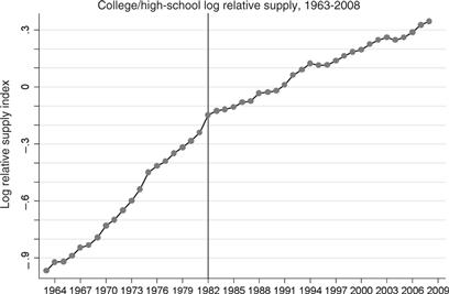
Figure 2 Source: March CPS data for earnings years 1963–2008. Labor supply is calculated using all persons aged 16–64 who reported having worked at least one week in the earnings years, excludingthosein the military. Thedata are sortedinto sex-education-experience groupsoftwo sexes (male/female), five education groups (high school dropout, high school graduate, some college, college graduate, and greater than college) and 49 experience groups (0–48 years of potential experience). The number of years of potential experience is calculated by subtracting the number six (the age at which one begins school) and the number of years of schooling from the age of the individual. This number is further adjusted using the assumption that an individual cannot begin work before age 16 and that experience is always non-negative. The labor supply for college/high school groups by experience level is calculated using efficiency units, equal to mean labor supply for broad college (including college graduates and greater than college) and high school (including high school dropouts and high school graduate) categories, weighted by fixed relative average wage weights for each cell. The labor supply of the “some college’’ category is allocated equally between the broad college and high school categories. The fixed set of wage weights for 1963–2008 are constructed using the average wage in each of the 490 cells (2 sexes, 5 education groups, 49 experience groups) over this time period.
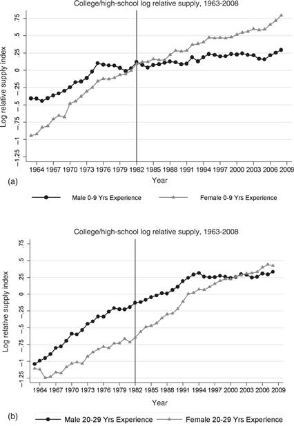
Figure 3 Source: March CPS data for earnings years 1963–2008. See note to Fig. 2. Log relative supply for 0–9 and 20–29years of potential experience is plotted for males and females.
What accounts for the deceleration of college relative supply in the 1980s? As discussed by Card and Lemieux (2001b), four factors seem particularly relevant. First, the Vietnam War artificially boosted college attendance during the late 1960s and early 1970s because males could in many cases defer military service by enrolling in post-secondary schooling. This deferral motive likely contributed to the acceleration of the relative supply of skills during the 1960s seen in Fig. 2. When the Vietnam War ended in the early 1970s, college enrollment rates dropped sharply, particularly among males, leading to a decline in college completion rates halfa decade later.
Second, the college premium declined sharply during the 1970s, as shown in Fig. 1. This downturn in relative college earnings likely discouraged high school graduates from enrolling in college. Indeed, Richard Freeman famously argued in his 1976 book, The Overeducated American, that the supply of college-educated workers in the United States had so far outstripped demand in the 1970s that the net social return to sending more high school graduates to college was negative.13
Third, the large baby boom cohorts that entered the labor market in the 1960s and 1970s were both more educated and more numerous than exiting cohorts, leading to a rapid increase in the average educational stock of the labor force. Cohorts born after 1964 were significantly smaller, and thus their impact on the overall educational stock of the labor force was also smaller. Had these cohorts continued the earlier trend in college-going behavior, their entry would still not have raised the college share of the workforce as rapidly as did earlier cohorts (see, e.g. Ellwood, 2002).
Finally, and most importantly, while the female college completion rate rebounded from its post-Vietnam era after 1980, the male college completion rate has never returned to its pre-1975 trajectory, as shown earlier in Fig. 3. While the data in that figure only cover the period from 1963 forward, the slow growth of college attainment is even more striking when placed against a longer historical backdrop. Between 1940 and 1980, the fraction of young adults aged 25 to 34 who had completed a four-year college degree at the start of each decade increased three-fold among both sexes, from 5 percent and 7 percent among females and males, respectively, in 1940 to 20 percent and 27 percent, respectively, in 1980. After 1980, however, this trajectory shifted differentially by sex. College completion among young adult females slowed in the 1980s but then rebounded in the subsequent two decades. Male college attainment, by contrast, peaked with the cohort that was age 25–34 in 1980. Even in 2008, it remained below its 1980 level. Cumulatively, these trends inverted the male to female gap in college completion among young adults. This gap stood at positive 7 percentage points in 1980 and negative 7 percentage points in 2008.
2.3. Real wage levels by skill group
A limitation of the college/high school wage premium as a measure of the market value of skill is that it necessarily omits information on real wage levels. Stated differently, a rising college wage premium is consistent with a rising real college wage, a falling real high school wage, or both. Movements in real as well as relative wages will prove crucial to our interpretation of the data. As shown formally in Section 3, canonical models used to analyze the college premium robustly predict that demand shifts favoring skilled workers will both raise the skill premium and boost the real earnings of all skill groups (e.g., college and high school workers). This prediction appears strikingly at odds with the data, as first reported by Katz and Murphy (1992), and shown in the two panels of Fig. 4. This figure plots the evolution of real log earnings by gender and education level for the same samples of full-time, full-year workers used above. Each series is normalized at zero in the starting year of 1963, with subsequent values corresponding to the log change in earnings for each group relative to its 1963 level. All values are deflated using the Personal Consumption Expenditure Deflator, produced by the US Bureau of Economic Analysis.
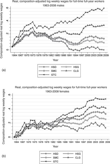
Figure 4 Source: March CPS data for earnings years 1963–2008. See note to Fig. 1. The real log weekly wage for each education group is the weighted average of the relevant composition adjusted cells using a fixed set of weights equal to the average employment share of each group. Nominal wage values are deflated using the Personal Consumption Expenditure (PCE) deflator.
In the first decade of the sample period, years 1963 through 1973, real wages rose steeply and relatively uniformly for both genders and all education groups. Log wage growth in this ten year period averaged approximately 20 percent. Following the first oil shock in 1973, wage levels fell sharply initially, and then stagnated for the remainder of the decade. Notably, this stagnation was also relatively uniform among genders and education groups. In 1980, wage stagnation gave way to three decades of rising inequality between education groups, accompanied by low overall rates of earnings growth—particularly among males. Real wages rose for highly educated workers, particularly workers with a post-college education, and fell steeply for less educated workers, particularly less educated males. Tables 1a and 1b provide many additional details on the evolution of real wage levels by sex, education, and experience groups during this period.
Table 1a
Changes in real, composition-adjusted log weekly wages for full-time, full-year workers, 1963–2008: by educational category and sex (100 × change in mean log real weekly wages).

Source: March CPS data for earnings years 1963–2008. See note to Fig. 1.
Table 1b
Changes in real, composition-adjusted log weekly wages for full-time, full-year workers, 1963–2008: by experience, educational category, and sex (100 × change in mean log real weekly wages).
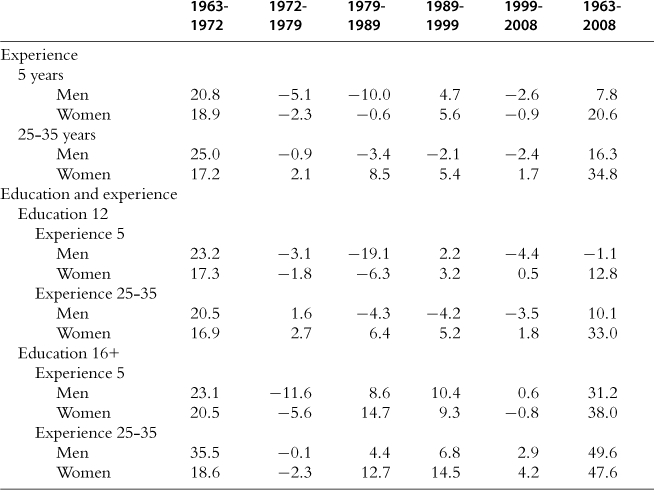
Source: March CPS data for earnings years 1963–2008. See note to Fig. 1.
Alongside these overall trends, Fig. 4 reveals three key facts about the evolution of earnings by education groups that are not evident from the earlier plots of the college/high school wage premium. First, a sizable share of the increase in college relative to non-college wages in 1980 forward is explained by the rising wages of post-college workers, i.e., those with post-baccalaureate degrees. Real earnings for this group increased steeply and nearly continuously from at least the early 1980s to present. By contrast, earnings growth among those with exactly a four-year degree was much more modest. For example, real wages of males with exactly a four-year degree rose 13 log points between 1979 and 2008, substantially less than they rose in only the first decade of the sample.
A second fact highlighted by Fig. 4 is that a major proximate cause of the growing college/high school earnings gap is not steeply rising college wages, but rapidly declining wages for the less educated–especially less educated males. Real earnings of males with less than a four year college degree fell steeply between 1979 and 1992, by 12 log points for high school and some-college males, and by 20 log points for high school dropouts. Low skill male wages modestly rebounded between 1993 and 2003, but never reached their 1980 levels. For females, the picture is qualitatively similar, but the slopes are more favorable. While wages for low skill males were falling in the 1980s, wages for low skill females were largely stagnant; when low skill males wages increased modestly in the 1990s, low skill female wages rose approximately twice as fast.
A potential concern with the interpretation of these results is that the measured real wage declines of less educated workers mask an increase in their total compensation after accounting for the rising value of employer provided non-wage benefits such as healthcare, vacation and sick time. Careful analysis of representative, wage and fringe benefits data by Pierce (2001, forthcoming) casts doubt on this notion, however. Monetizing the value of these benefits does not substantially alter the conclusion that real compensation for low skilled workers fell in the 1980s. Further, Pierce shows that total compensation—that is, the sum of wages and in-kind benefits—for high skilled workers rose by more than their wages, both in absolute terms and relative to compensation for low skilled workers.14 A complementary analysis of the distribution of non-wage benefits—including safe working conditions and daytime versus night and weekend hours—by Hamermesh (1999) also reaches similar conclusions. Hamermesh demonstrates that trends in the inequality of wages understate the growth in full earnings inequality (i.e., absent compensating differentials) and, moreover, that accounting for changes in the distribution of non-wage amenities augments rather than offsets changes in the inequality of wages. It is therefore unlikely that consideration of non-wage benefits changes the conclusion that low skill workers experienced significant declines in their real earnings levels during the 1980s and early 1990s.15
The third key fact evident from Fig. 4 is that while the earnings gaps between some-college, high school graduate, and high school dropout workers expanded sharply in the 1980s, these gaps stabilized thereafter. In particular, the wages of high school dropouts, high school graduates, and those with some college moved largely in parallel from the early 1990s forward.
The net effect of these three trends—rising college and post-college wages, stagnant and falling real wages for those without a four-year college degree, and the stabilization of the wage gaps among some-college, high school graduates, and high school dropout workers—is that the wage returns to schooling have become increasingly convex in years of education, particularly for males, as emphasized by Lemieux (2006b). Figure 5 shows this “convexification” by plotting the estimated gradient relating years of educational attainment to log hourly wages in three representative years of our sample: 1973, 1989, and 2009. To construct this figure, we regress log hourly earnings in each year on a quadratic in years of completed schooling and a quartic in potential experience. Models that pool males and females also include a female main effect and an interaction between the female dummy and a quartic in (potential) experience.16 In each figure, the predicted log earnings of a worker with seven years of completed schooling and 25 years of potential experience in 1973 is normalized to zero. The slope of the 1973 locus then traces out the implied log earnings gain for each additional year of schooling in 1973, up to 18 years. The loci for 1989 and 2009 are constructed similarly, and they are also normalized relative to the intercept in 1973. This implies that upward or downward shifts in the intercepts of these loci correspond to real changes in log hourly earnings, whereas rotations of the loci indicate changes in the education-wage gradient.17
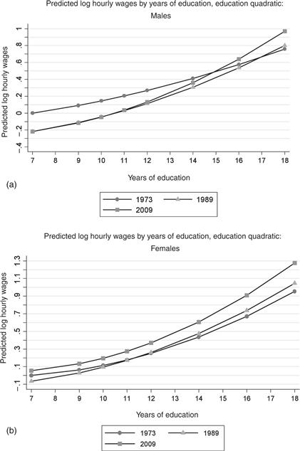
Figure 5 Source: May/ORG CPS data for earnings years 1973–2009. For each year, log hourly wages for all workers, excluding the self-employed and those employed by the military, are regressed on a quadratic in education (eight categories), a quartic in experience, a female dummy, and interactions of the female dummy and the quartic in experience. Predicted real log hourly wages are computed in 1973, 1989 and2009 for each of the years of schooling presented in the figure. See the Data Appendix for more details on the treatment of May/ORG CPS data.
The first panel of Fig. 5 shows that the education-wage gradient for males was roughly log linear in years of schooling in 1973, with a slope approximately equal to 0.07 (that is, 7 log points of hourly earnings per year of schooling). Between 1973 and 1989, the slope steepened while the intercept fell by a sizable 10 log points. The crossing point of the two series at 16 years of schooling implies that earnings for workers with less than a four-year college degree fell between 1973 and 1989, consistent with the real wage plots in Fig. 4. The third locus, corresponding to 2009, suggests two further changes in wage structure in the intervening two decades: earnings rose modestly for low education workers, seen in the higher 2009 intercept (though still below the 1973 level); and the locus relating education to earnings became strikingly convex. Whereas the 1989 and 2009 loci are roughly parallel for educational levels below 12, the 2009 locus is substantially steeper above this level. Indeed at 18 years of schooling, it lies 16 log points above the 1989 locus. Thus, the return to schooling first steepened and then “convexified” between 1973 and 2009.
Panel B of Fig. 5 repeats this estimation for females. The convexification of the return to education is equally apparent for females, but the downward shift in the intercept is minimal. These differences by gender are, of course, consistent with the differential evolution of wages by education group and gender shown in Fig. 4.
As a check to ensure that these patterns are not driven by the choice of functional form, Fig. 6 repeats the estimation, in this case replacing the education quartic with a full set of education dummies. While the fitted values from this model are naturally less smooth than in the quadratic specification, the qualitative story is quite similar: between 1973 and 1989, the education-wage locus intercept falls while the slope steepens. The 1989 curve crosses the 1973 curve at 18 years of schooling. Two decades later, the education-wage curve lies atop the 1989 curve at low years of schooling, while it is both steeper and more convex for completed schooling beyond the 12th year.
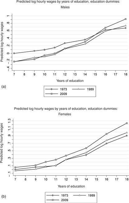
Figure 6 Source: May/ORG CPS data for earnings years 1973–2009. For each year, log hourly wages for all workers, excluding the self-employed and those employed by the military, are regressed on eight education dummies, a quartic in experience, a female dummy, and interactions of the female dummy and the quartic in experience. Predicted real log hourly wages are computed in 1973, 1989 and 2009 for each of the years of schooling presented. See the Data Appendix for more details on the treatment of May/ORG CPS data.
2.4. Overall wage inequality
Our discussion so far summarizes the evolution of real and relative wages by education, gender and experience groups. It does not convey the full set of changes in the wage distribution, however, since there remains substantial wage dispersion within as well as between skill groups. To fill in this picture, we summarize changes throughout the entire earnings distribution. In particular, we show the trends in real wages by earnings percentile, focusing on the 5th through 95th percentiles of the wage distribution. We impose this range restriction because the CPS and Census samples are unlikely to provide accurate measures of earnings at the highest and lowest percentiles. High percentiles are unreliable both because high earnings values are truncated in public use samples and, more importantly, because non-response and under-reporting are particularly severe among high income households.18 Conversely, wage earnings in the lower percentiles imply levels of consumption that lie substantially below observed levels (Meyer and Sullivan, 2008). This disparity reflects a combination of measurement error, underreporting, and transfer income among low wage individuals.
Figure 7 plots the evolution of real log weekly wages of full-time, full-year workers at the 10th, 50th and 90th percentiles of the earnings distribution from 1963 through 2008. In each panel, the value of the 90th, 50th and 10th percentiles are normalized to zero in the start year of 1963, with subsequent data points measuring log changes from this initial level. Many features of Fig. 7 closely correspond to the education by gender real wages series depicted in Fig. 4. For both genders, the 10th, 50th and 90th percentiles of the distribution rise rapidly and relatively evenly between 1963 and 1973. After 1973, the 10th and 50th percentiles continue to stagnate relatively uniformly for the remainder of the decade. The 90th percentile of the distribution pulls away modestly from the median throughout the decade of the 1970s, echoing the rise in earnings among post-college workers in that decade.19
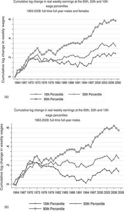
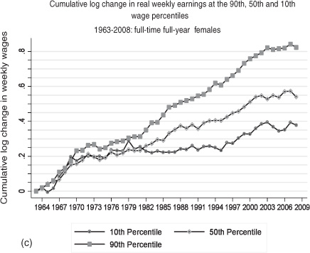
Figure 7 Source: March CPS data for earnings years 1963–2008. For each year, the 10th, median and 90th percentiles of log weekly wages are calculated for full-time, full-year workers.
Reflecting the uneven distribution of wage gains by education group, growth in real earnings among males occurs among high earners, but is not broadly shared. This is most evident by comparing the male 90th percentile with the median. The 90th percentile rose steeply and almost monotonically between 1979 and 2007. By contrast, the male median was essentially flat from 1980 to 1994. Simultaneously, the male 10th percentile fell steeply (paralleling the trajectory of high school dropout wages). When the male median began to rise during the mid 1990s (a period of rapid productivity and earnings growth in the US economy), the male 10th percentile rose concurrently and slightly more rapidly. This partly reversed the substantial expansion of lower-tail inequality that unfolded during the 1980s.
The wage picture for females is qualitatively similar, but the steeper slopes again show that the females have fared better than males during this period. As with males, the growth of wage inequality is asymmetric above and below the median. The female 90/50 rises nearly continuously from the late 1970s forward. By contrast, the female 50/10 expands rapidly during the 1980s, plateaus through the mid-1990s, and then compresses modestly thereafter.
Because Fig. 7 depicts wage trends for full-time, full-year workers, it tends to obscure wage developments lower in the earnings distribution, where a larger share of workers are part-time or part-year. To capture these developments, we apply the May/ORG CPS log hourly wage samples for years 1973 through 2009 (i.e., all available years) to plot in Fig. 8 the corresponding trends in real indexed hourly wages of all employed workers at the 10th, 50th, and 90th percentiles. Due to the relatively small size of the May sample, we pool three years of data at each point to increase precision (e.g., plotted year 1974 uses data from 1973, 1974 and 1975).
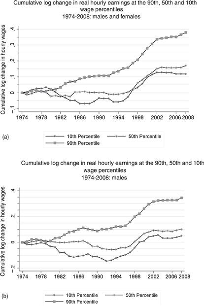
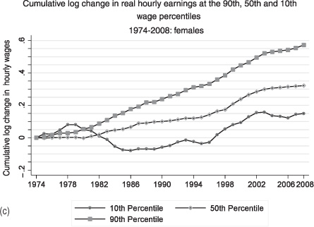
Figure 8 Source: May/ORG CPS data for earnings years 1973–2009. The data are pooled using three-year moving averages (i.e. the year 1974 includes data from years 1973,1974 and 1975). For each year, the 10th, median and 90th percentiles of log weekly wages are calculated for all workers, excluding the self-employed and those employed in military occupations.
The additional fact revealed by Fig. 8 is that downward movements at the 10th percentile are far more pronounced in the hourly wage distribution than in the full-time weekly data. For example, the weekly data show no decline in the female 10th percentile between 1979 and 1986, whereas the hourly wage data show a fall of 10 log points in this period.20 Similarly, the modest closing of the 50/10 earnings gap after 1995 seen in the full-time, full-year sample is revealed as a sharp reversal of the 1980s expansion of 50/10 wage inequality in the full hourly distribution. Thus, the monotone expansion in the 1980s of wage inequality in the top and bottom halves of the distribution became notably non-monotone during the subsequent two decades.21
The contrast between these two periods of wage structure changes—one monotone, the other non-monotone—is shown in stark relief in Fig. 9, which plots the change at each percentile of the hourly wage distribution relative to the corresponding median during two distinct eras, 1974–1988 and 1988–2008. The monotonicity of wage structure changes during the first period, 1974–1988, is immediately evident for both genders.22 Equally apparent is the U-shaped (or “polarized”) growth of wages by percentile in the 1988–2008 period, which is particularly evident for males. The steep gradient of wage changes above the median is nearly parallel, however, for these two time intervals. Thus, the key difference between the two periods lies in the evolution of the lower-tail, which is falling steeply in the 1980s and rising disproportionately at lower percentiles thereafter.23
Though the decade of the 2000s is not separately plotted in Fig. 9, it bears note that the U-shaped growth of hourly wages is most pronounced during the period of 1988 through 1999. For the 1999 through 2007 interval, the May/ORG data show a pattern of wage growth that is roughly flat across the first seven deciles of the distribution, and then upwardly sloped in the three highest deciles, though the slope is shallower than in either of the prior two decades.
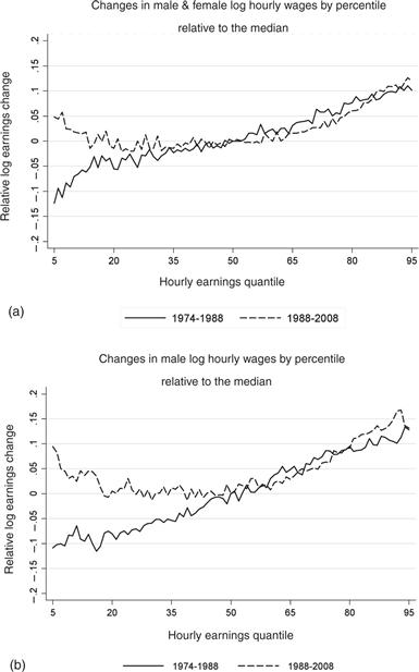
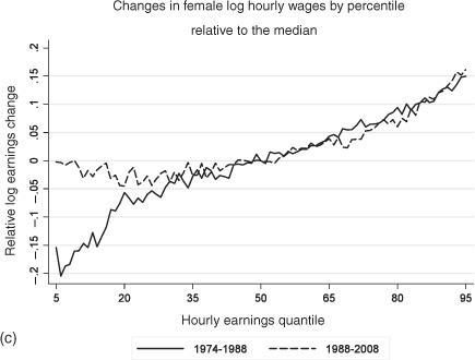
Figure 9 Source: May/ORG CPS data for earnings years 1973–2009. The data are pooled using three-year moving averages (i.e. the year 1974 includes data from years 1973, 1974 and 1975). For each year, the 5th through 95th percentiles of log hourly wages are calculated for all workers, excluding the self-employed and those employed in military occupations. The log wage change at the median is normalized to zero in each time interval.
These divergent trends in upper-tail, median and lower-tail earnings are of substantial significance for our discussion, and we consider their causes carefully below. Most notable is the “polarization” of wage growth—by which we mean the simultaneous growth of high and low wages relative to the middle—which is not readily interpretable in the canonical two factor model. This polarization is made more noteworthy by the fact that the return to skill, measured by the college/high school wage premium, rose monotonically throughout this period, as did inequality above the median of the wage distribution. These discrepancies between the monotone rise of skill prices and the nonmonotone evolution of inequality again underscore the potential utility of a richer model of wage determination.
Substantial changes in wage inequality over the last several decades are not unique to the US, though neither is the US a representative case. Summarizing the literature circa ten years ago, Katz and Autor (1999) report that most industrialized economies experienced a compression of skill differentials and wage inequality during the 1970s, and a modest to large rise in differentials in the 1980s, with the greatest increase seen in the US and UK. Drawing on more recent and consistent data for 19 OECD countries, Atkinson reports that there was at least a five percent increase in either upper-tail or lower-tail inequality between 1980 and 2005 in 16 countries, and a rise of at least 5 percent in both tails in seven countries. More generally, Atkinson notes that substantial rises in upper-tail inequality are widespread across OECD countries, whereas movements in the lower-tail vary more in sign, magnitude, and timing.24
2.5. Job polarization
Accompanying the wage polarization depicted in Fig. 7 through 9 is a marked pattern of job polarization in the United States and across the European Union—by which we mean the simultaneous growth of the share of employment in high skill, high wage occupations and low skill, low wage occupations. We begin by depicting this broad pattern (first noted in Acemoglu, 1999) using aggregate US data. We then link the polarization of employment to the “routinization” hypothesis proposed by Autor et al., (2003“ALM” hereafter), and we explore detailed changes in occupational structure across the US and OECD in light of that framework.
Changes in occupational structure
Figure 10 provides a starting point for the discussion of job polarization by plotting the change over each of the last three decades in the share of US employment accounted for by 318 detailed occupations encompassing all of US employment. These occupations are ranked on the x-axis by their skill level from lowest to highest, where an occupation’s skill rank is approximated by the average wage of workers in the occupation in 1980.25 The y-axis of the figure corresponds to the change in employment at each occupational percentile as a share of total US employment during the decade. Since the sum of shares must equal one in each decade, the change in these shares across decades must total zero. Thus, the height at each skill percentile measures the growth in each occupation’s employment relative to the whole.26
The figure reveals a pronounced “twisting” of the distribution of employment across occupations over three decades, which becomes more pronounced in each period. During the 1980s (1979–1989), employment growth by occupation was nearly monotone in occupational skill; occupations below the median skill level declined as a share of employment and occupations above the median increased. In the subsequent decade, this monotone relationship gave way to a distinct pattern of polarization. Relative employment growth was most rapid at high percentiles, but it was also modestly positive at low percentiles (10th percentile and down) and modestly negative at intermediate percentiles. In contrast, during the most recent decade for which Census/ACS data are available, 1999–2007, employment growth was heavily concentrated among the lowest three deciles of occupations. In deciles four through nine, the change in employment shares was negative, while in the highest decile, almost no change is evident. Thus, the disproportionate growth of low education, low wage occupations became evident in the 1990s and accelerated thereafter.27
This pattern of employment polarization is not unique to the United States, as is shown in Fig. 11. This figure, based on Table 1 of Goos et al. (2009), depicts the change in the share of overall employment accounted for by three sets of occupations grouped according to average wage level—low, medium, and high—in each of 16 European Union countries during the period 1993 through 2006.28 Employment polarization is pronounced across the EU during this period. In all 16 countries depicted, middle wage occupations decline as a share of employment. The largest declines occur in France and Austria (by 12 and 14 percentage points, respectively) and the smallest occurs in Portugal (1 percentage point). The unweighted average decline in middle skill employment across countries is 8 percentage points.
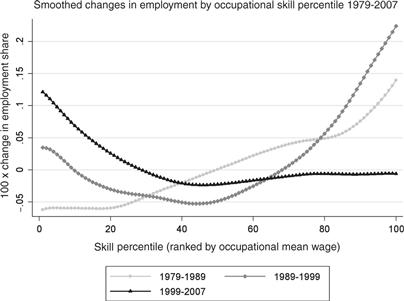
Figure 10 Source: Census IPUMS 5 percent samples for years 1980, 1990, and 2000, and Census American Community Survey for 2008. All occupation and earnings measures in these samples refer to prior year’s employment. The figure plots log changes in employment shares by 1980 occupational skill percentile rank using a locally weighted smoothing regression (bandwidth 0.8 with 100 observations), where skill percentiles are measured as the employment-weighted percentile rank of an occupation’s mean log wage in the Census IPUMS 1980 5 percent extract. The mean log wage in each occupation is calculated using workers’ hours of annual labor supply times the Census sampling weights. Consistent occupation codes for Census years 1980, 1990, and 2000, and 2008 are from Autor and Dorn (2009).
The declining share of middle wage occupations is offset by growth in high and low wage occupations. In 13 of 16 countries, high wage occupations increased their share of employment, with an average gain of 6 percentage points, while low wage occupations grew as a share of employment in 11 of 16 countries. Notably, in all 16 countries, low wage occupations increased in size relative to middle wage occupations, with a mean gain in employment in low relative to middle wage occupations of 10 percentage points.
For comparison, Fig. 11 also plots the unweighted average change in the share of national employment in high, middle, and low wage occupations in all 16 European Union economies alongside a similar set of occupational shift measures for the United States. Job polarization appears to be at least as pronounced in the European Union as in the United States.
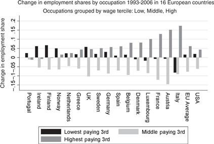
Figure 11 Source: Data on EU employment are from Goos et al. (2009). US data are from the May/ORG CPS files for years 1993–2006. The data include all persons aged 16–64 who reported employment in the sample reference week, excluding those employed by the military and in agricultural occupations. Occupations are first assigned to 326 occupation groups that are consistent over the given time period. These occupations are then grouped into three broad categories by wage level.
Figure 12 studies the specific changes in occupational structure that drive job polarization in the United States. The figure plots percentage point changes in employment levels by decade for the years 1979–2009 for 10 major occupational groups encompassing all of US non-agricultural employment. We use the May/ORG data so as to include the two recession years of 2007 through 2009 (separately plotted).29
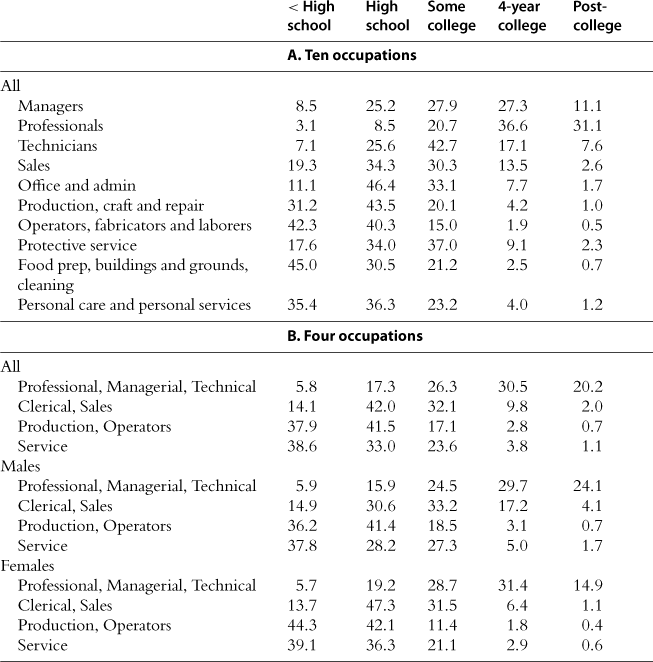
The 10 occupations summarized in Fig. 12 divide neatly into three groups. On the left-hand side of the figure are managerial, professional and technical occupations. These are highly educated and highly paid occupations. Between one-quarter and two-thirds of workers in these occupations had at least a four-year college degree in 1979, with the lowest college share in technical occupations and the highest in professional occupations (Table 4). Employment growth in these occupations was robust throughout the three decades plotted. Even in the deep recession of 2007 through 2009, during which the number of employed US workers fell by approximately 8 million, these occupations experienced almost no absolute decline in employment.
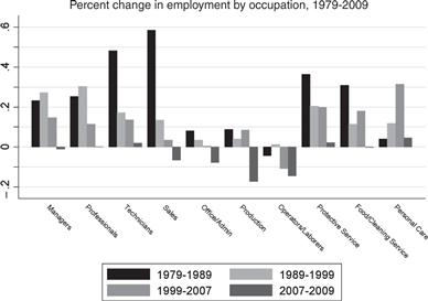
Figure 12 Source: May/ORG CPS files for earnings years 1979–2009. The data include all persons aged 16–64 who reported employment in the sample reference week, excluding those employed by the military and in agricultural occupations. Occupations are assigned to 326 occupation groups that are consistent over the given time period. All non-military, non-agricultural occupations are assigned to one often broad occupations presented in the figure.
Table 4
Education distribution by occupation and gender in 1979 (Census data).
Source: Census IPUMS 5 percent samples for years 1960, 1970, 1980, 1990, and 2000, and Census American Community Survey for 2008. See note to Tables 3a and 3b.
The subsequent four columns display employment growth in “middle skill occupations,” which we define as comprising sales; office and administrative support; production, craft and repair; and operator, fabricator and laborer. The first two of this group of four are middle skilled, white-collar occupations that are disproportionately held by women with a high school degree or some college. The latter two categories are a mixture of middle and low skilled blue-collar occupations that are disproportionately held by males with a high school degree or lower education. While the headcount in these occupations rose in each decadal interval between 1979–2007, their growth rate lagged the economy-wide average and, moreover, generally slowed across decades. These occupations were hit particularly hard during the 2007–2009 recession, with absolute declines in employment ranging from 7 to 17 percent.
The last three columns of Fig. 12 depict employment trends in service occupations, which are defined by the Census Bureau as jobs that involve helping, caring for or assisting others. The majority of workers in service occupations have no post-secondary education, and average hourly wages in service occupations are in most cases below the other seven occupations categories. Despite their low educational requirements and low pay, employment growth in service occupations has been relatively rapid over the past three decades. Indeed, Autor and Dorn (2010) show that rising service occupation employment accounts almost entirely for the upward twist of the lower tail of Fig. 10 during the 1990s and 2000s. All three broad categories of service occupations— protective service, food preparation and cleaning services, and personal care—expanded by double digits in both the 1990s and the pre-recession years of the past decade (1999–2007). Protective service and food preparation and cleaning occupations expanded even more rapidly during the 1980s. Notably, even during the recessionary years of 2007 through 2009, employment growth in service occupations was modestly positive—more so, in fact, than the three high skilled occupations that have also fared comparatively well (professional, managerial and technical occupations). As shown in Tables 3a and 3b, the employment share of service occupations was essentially flat between 1959 and 1979. Thus, their rapid growth since 1980 marks a sharp trend reversal.
Table 3a
Employment shares in four broad occupational categories (%), 1959–2007.
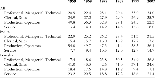
Source: Census IPUMS 5 percent samples for years 1960, 1970, 1980, 1990, and 2000, and Census American Community Survey for 2008. See note to Fig. 13.
Table 3b
Mean log full-time, full-year weekly and all hourly earnings in four broad occupation categories, 1959–2007 (Census) and 1973–2009 (May/ORG).
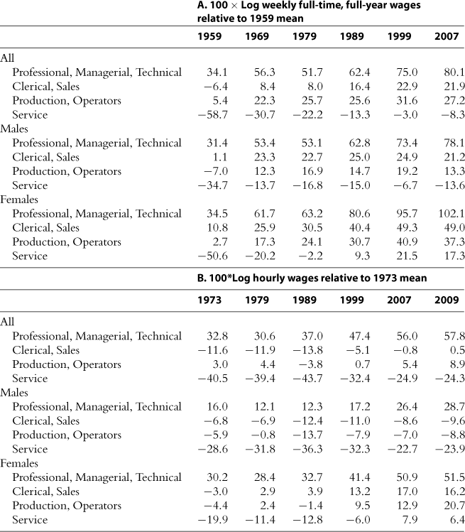
Source: Census IPUMS 5 percent samples for years 1960, 1970, 1980, 1990, and 2000, and Census American Community Survey for 2008. May/ORG CPS data for earnings years 1973–2009. See note to Fig. 13.
Cumulatively, these two trends—rapid employment growth in both high and low education jobs—have substantially reduced the share of employment accounted for by “middle skill” jobs. In 1979, the four middle skill occupations—sales, office and administrative workers, production workers, and operatives—accounted for 57.3 percent of employment. In 2007, this number was 48.6 percent, and in 2009, it was 45.7 percent. One can quantify the consistency of this trend by correlating the growth rates of these occupation groups across multiple decades. The correlation between occupational growth rates in 1979–1989 and 1989–1999 is 0.53, and for the decades of 1989–1999 and 1999–2009, it is 0.74. Remarkably, the correlation between occupational growth rates during 1999–2007 and 2007–2009—that is, prior to and during the current recession— is 0.76.30
Sources of job polarization: The “routinization” hypothesis
Autor et al. (2003) link job polarization to rapid improvements in the productivity—and declines in the real price—ofinformation and communications technologies and, more broadly, symbolic processing devices. ALM take these advances as exogenous, though our framework below shows how they can also be understood as partly endogenous responses to changes in the supplies of skills. ALM also emphasize that to understand the impact of these technical changes on the labor market, is necessary to study the “tasks content” of different occupations. As already mentioned in the Introduction, and as we elaborate further below, a task is a unit of work activity that produces output (goods and services), and we think of workers as allocating their skills to different tasks depending on labor market prices.
While the rapid technological progress in information and communications technology that motivates the ALM paper is evident to anyone who owns a television, uses a mobile phone, drives a car, or takes a photograph, its magnitude is nevertheless stunning. Nordhaus (2007) estimates that the real cost of performing a standardized set of computational tasks—where cost is expressed in constant dollars or measured relative to the labor cost of performing the same calculations—fell by at least 1.7 trillion-fold between 1850 and 2006, with the bulk of this decline occurring in the last three decades. Of course, the progress of computing was almost negligible from 1850 until the era of electromechanical computing (i.e., using relays as digital switches) at the outset of the twentieth century. Progress accelerated during World War II, when vacuum tubes replaced relays. Then, when microprocessors became widely available in the 1970s, the rate of change increased discontinuously. Nordhaus estimates that between 1980 and 2006, the real cost of performing a standardized set of computations fell by 60 to 75 percent annually. Processing tasks that were unthinkably expensive 30 years ago—such as searching the full text of a university’s library for a single quotation—became trivially cheap.
The rapid, secular price decline in the real cost of symbolic processing creates enormous economic incentives for employers to substitute information technology for expensive labor in performing workplace tasks. Simultaneously, it creates significant advantages for workers whose skills become increasingly productive as the price of computing falls. Although computers are now ubiquitous, they do not do everything. Computers—or, more precisely, symbolic processors that execute stored instructions— have a very specific set of capabilities and limitations. Ultimately, their ability to accomplish a task is dependent upon the ability of a programmer to write a set of procedures or rules that appropriately direct the machine at each possible contingency. For a task to be autonomously performed by a computer, it must be sufficiently well defined (i.e., scripted) that a machine lacking flexibility or judgment can execute the task successfully by following the steps set down by the programmer. Accordingly, computers and computer-controlled equipment are highly productive and reliable at performing the tasks that programmers can script—and relatively inept at everything else. Following, ALM, we refer to these procedural, rule-based activities to which computers are currently well-suited as “routine” (or “codifiable”) tasks. By routine, we do not mean mundane (e.g., washing dishes) but rather sufficiently well understood that the task can be fully specified as a series of instructions to be executed by a machine (e.g., adding a column of numbers).
Routine tasks are characteristic of many middle skilled cognitive and manual jobs, such as bookkeeping, clerical work, repetitive production, and monitoring jobs. Because the core job tasks of these occupations follow precise, well-understood procedures, they can be (and increasingly are) codified in computer software and performed by machines (or, alternatively, are sent electronically—”outsourced”—to foreign worksites). The substantial declines in clerical and administrative occupations depicted in Fig. 12 are likely a consequence of the falling price of machine substitutes for these tasks. It is important to observe, however, that computerization has not reduced the economic value or prevalence of the tasks that were performed by workers in these occupations—quite the opposite.31 But tasks that primarily involve organizing, storing, retrieving, and manipulating information—most common in middle skilled administrative, clerical and production tasks—are increasingly codified in computer software and performed by machines.32 Simultaneously, these technological advances have dramatically lowered the cost of offshoring information-based tasks to foreign worksites (Blinder, 2007; Jensen et al., 2005; Jensen and Kletzer, forthcoming; Blinder and Krueger, 2008; Oldenski, 2009).33
This process of automation and offshoring of routine tasks, in turn, raises relative demand for workers who can perform complementary non-routine tasks. In particular, ALM argue that non-routine tasks can be roughly subdivided into two major categories: abstract tasks and manual tasks (two categories that lie at opposite ends of the occupational-skill distribution). Abstract tasks are activities that require problem-solving, intuition, persuasion, and creativity. These tasks are characteristic of professional, managerial, technical and creative occupations, such as law, medicine, science, engineering, design, and management, among many others. Workers who are most adept in these tasks typically have high levels of education and analytical capability. ALM further argue that these analytical tasks are complementary to computer technology, because analytic, problem-solving, and creative tasks typically draw heavily on information as an input. When the price of accessing, organizing, and manipulating information falls, abstract tasks are complemented.
Non-routine manual tasks are activities that require situational adaptability, visual and language recognition, and in-person interactions. Driving a truck through city traffic, preparing a meal, installing a carpet, or mowing a lawn are all activities that are intensive in non-routine manual tasks. As these examples suggest, non-routine manual tasks demand workers who are physically adept and, in some cases, able to communicate fluently in spoken language. In general, they require little in the way of formal education relative to a labor market where most workers have completed high school.
This latter observation applies with particular force to service occupations, as stressed by Autor and Dorn (2009, 2010). Jobs such as food preparation and serving, cleaning and janitorial work, grounds cleaning and maintenance, in-person health assistance by home health aides, and numerous jobs in security and protective services, are highly intensive in non-routine manual tasks. The core tasks of these jobs demand interpersonal and environmental adaptability. These are precisely the job tasks that are challenging to automate because they require a level of adaptability and responsiveness to unscripted interactions—both with the environment and with individuals—which at present exceed the limits of machine-competency, though this will surely change in the long run. It also bears note that these same job tasks are infeasible to offshore in many cases because they must be produced and performed in person (again, for now). Yet, these jobs generally do not require formal education beyond a high school degree or, in most cases, extensive training.34
In summary, the displacement of jobs that are intensive in routine tasks may have contributed to the polarization of employment by reducing job opportunities in middle skilled clerical, administrative, production and operative occupations. Jobs that are intensive in either abstract or non-routine manual tasks, however, are much less susceptible to this process due to the demand for problem-solving, judgment and creativity in the former case, and flexibility and physical adaptability in the latter. Since these jobs are found at opposite ends of the occupational skill spectrum—in professional, managerial and technical occupations on the one hand, and in service and laborer occupations on the other—the consequence may be a partial “hollowing out” or polarization of employment opportunities. We formalize these ideas in the model below.35
Linking occupational changes to job tasks
Drawing on this task-based conceptual framework, we now explore changes in occupational structure in greater detail. To make empirical progress on the analysis of job tasks, we must be able to characterize the “task content” of jobs. In their original study of the relationship between technological change and job tasks, ALM used the US Department of Labor’s Dictionary of Occupational Titles (DOT) to impute to workers the task measures associated with their occupations. This imputation approach has the virtue of distilling the several hundred occupational titles found in conventional data sources into a relatively small number of task dimensions. A drawback, however, is that both the DOT, and its successor, the Occupational Information Network (O*NET), contain numerous potential task scales, and it is rarely obvious which measure (ifany) best represents a given task construct. Indeed, the DOT contains 44 separate scales, and the O*NET contains 400, which exceeds the number of unique Census occupation codes found in the CPS, Census, and ACS data sets.36
To skirt these limitations and maximize transparency in this chapter, we proxy for job tasks here by directly working with Census and CPS occupational categories rather than imputing task data to these categories. To keep categories manageable and self-explanatory, we use broad occupational groupings, either at the level of the ten categories as in Fig. 12—ranging from Managers to Personal Care workers—or even more broadly, at the level of the four clusters that are suggested by the figure: (1) managerial, professional and technical occupations; (2) sales, clerical and administrative support occupations; (3) production, craft, repair, and operative occupations; and (4) service occupations. Though these categories are coarse, we believe they map logically into the broad task clusters identified by the conceptual framework. Broadly speaking, managerial, professional, and technical occupations are specialized in abstract, non-routine cognitive tasks; clerical, administrative and sales occupations are specialized in routine cognitive tasks; production and operative occupations are specialized in routine manual tasks; and service occupations are specialized in non-routine manual tasks.
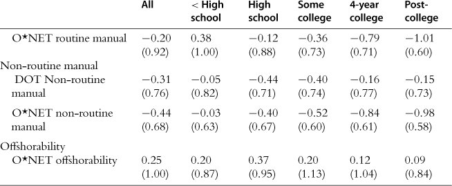
Before turning to the occupational analysis, we use data from both the DOT and O*NET to verify that our heuristic characterization of the major task differences across these broad occupational groups is supported. The task measures from the DOT, presented in Tables 5a and 5b, were constructed by ALM (2003) and have subsequently been widely used in the literature.37 The companion set of O*NET task measures in the table are new to this chapter. Since the O*NET is the successor data source to the DOT, the O*NET based measures are potentially preferable. However, the O*NET’s large set of loosely defined and weakly differentiated scales present challenges for researchers.38
Table 5a
Means and standard deviations of DOT and O*NETtask measures for four broad occupational groups in 1980 Census.
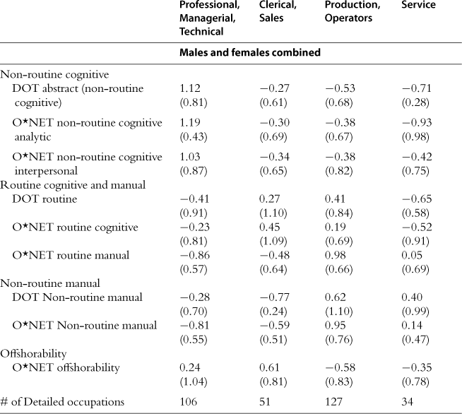
Source: O*NET and DOT. Task measures are constructed according to the procedure in the Data Appendix.
Table 5b
Means and standard deviations of DOT and O*NET task measures by education level in 1979 Census.
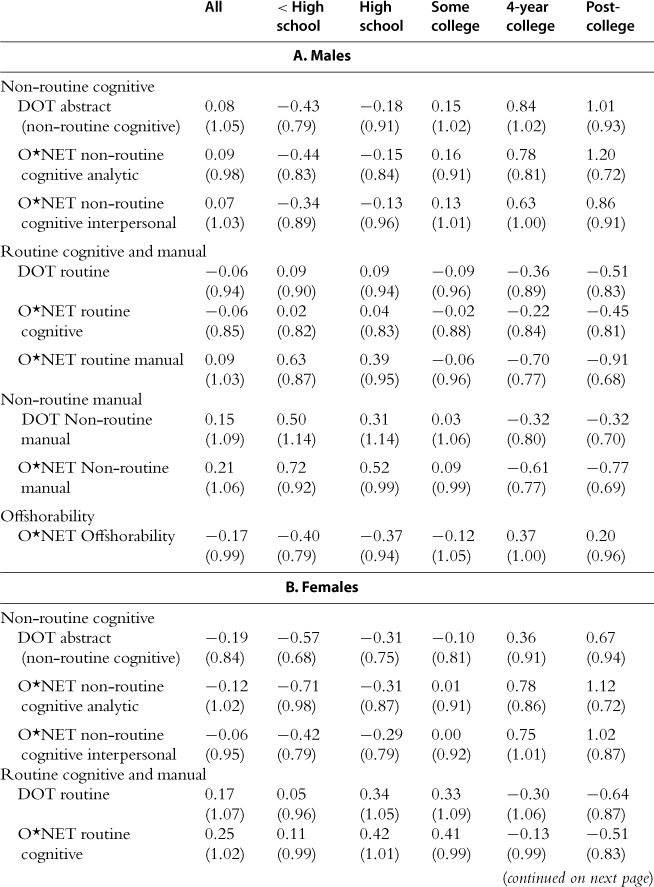
Source: O*NET and DOT. Task measures are constructed according to the procedure in the Data Appendix.
Consistent with expectations, Table 5a shows that the intensity of use of nonroutine cognitive (“abstract”) tasks is highest in professional, technical and managerial occupations, and lowest in service and laborer occupations. To interpret the magnitudes of these differences, note that all task measures in Tables 5a and 5b are standardized to have a mean of zero and a cross-occupation standard deviation of one in 1980 across the 318 consistently coded occupations used in our classification.39 Thus, the means of −0.67 and 1.22, respectively, for service occupations and professional, managerial and technical occupations indicate approximately a two standard deviation (–0.67 − 1.22 ![]() 2) average gap in abstract task intensity between these occupational groups. The subsequent two rows of the table present a set of O*NET-based measures of abstract task input. Our O*NET task measures also make a further distinction between non-routine cognitive analytic tasks (e.g., mathematics and formal reasoning) and non-routine cognitive interpersonal and managerial tasks. The qualitative pattern of task intensity across the occupation groups is comparable for the two measures and also similar to the DOT non-routine cognitive (abstract) task measure.
2) average gap in abstract task intensity between these occupational groups. The subsequent two rows of the table present a set of O*NET-based measures of abstract task input. Our O*NET task measures also make a further distinction between non-routine cognitive analytic tasks (e.g., mathematics and formal reasoning) and non-routine cognitive interpersonal and managerial tasks. The qualitative pattern of task intensity across the occupation groups is comparable for the two measures and also similar to the DOT non-routine cognitive (abstract) task measure.
The next three rows of the table present measures of routine task intensity. Distinct from abstract tasks, routine task intensity is non-monotone in occupational “skill” level, with the highest levels of routine-intensity found in clerical/sales occupations and production/operative occupations. Using the O*NET, we make a further distinction between routine cognitive and routine manual tasks. Logically, routine cognitive tasks are most intensively used in clerical and sales occupations and routine manual tasks are most prevalent in production and operative positions. Finally, non-routine manual tasks—those requiring flexibility and physical adaptability—are most intensively used in production, operative and service positions.
Blinder (2007) and Blinder and Krueger (2008) have argued that essentially any job that does not need to be done in person (i.e., face-to-face) can ultimately be outsourced, regardless of whether its primary tasks are abstract, routine, or manual. Tables 5a and 5b also provide a measure of occupational off shorability. This measure codes the degree to which occupations require face-to-face interactions, demand on-site presence (e.g., constructing a house), or involve providing in-person care to others.40 As with routine tasks, off shorability is highest in clerical/sales occupations. Unlike the routine measure, however, off shorability is considerably higher in professional, managerial and technical occupations than in either production/operative or in service occupations, reflecting the fact that many white-collar job tasks primarily involve generating, processing, or providing information, and so can potentially be performed from any location.
Table 5b summarizes task intensity by education group and sex. Logically, both abstract and manual tasks are monotone in educational level, the former increasing in education and the latter decreasing. Routine cognitive tasks are strongly non-monotone in education, however. They are used most intensively by high school and some-college workers, and are substantially higher on average among women than men (reflecting female specialization in administrative and clerical occupations). Routine manual tasks, in turn, are substantially higher among males, reflecting male specialization in blue collar production and operative occupations.
Notably, the off shorability index indicates that the jobs performed by women are on average substantially more suitable to offshoring than those performed by males. Moreover, the educational pattern of off shorability also differs by sex. High school females are most concentrated in potentially off shorable tasks, while for males, college graduates are most often found in off shorable tasks. This pattern reflects the fact that among non-college workers, females are more likely than males to hold clerical, administrative and sales occupations (which are relatively off shorable), while males are far more likely than females to hold blue collar jobs (which are relatively non-offshorable).
These patterns of specialization appear broadly consistent with our characterization of the task content of broad occupational categories: professional, managerial and technical occupations are specialized in non-routine cognitive tasks; clerical and sales occupations are specialized in routine cognitive tasks; production and operative occupations are specialized in routine manual tasks; and service occupations are specialized in nonroutine manual tasks. Although all occupations combine elements from each task category, and moreover, task intensity varies among detailed occupations within these broad groups (and among workers in these occupations), we suspect that these categories capture the central tendencies of the data and also provide a useful mnemonic for parsing the evolution of job task structure.
The evolution of job tasks
In Figs 13 and 14, we study the evolution of employment among these four broad task/occupation categories, starting with overall shifts in employment across occupational categories between 1959 and 2007 (Fig. 13). Most evident in this figure is the secular growth of professional, managerial, and technical occupations and the secular decline of production and operative positions. Among males, blue-collar and production and operative employment fell by nearly 20 percentage points between 1959 and 1979 (from 54.0 to 36.1 percent). The two categories that absorbed this slack are professional, managerial and technical occupations and, after 1979, service occupations. Figure 14 further shows that service occupation employment rose rapidly among males with less than a four-year college degree after 1979, and most rapidly in the current decade. In net, the share of males employed in service occupations rose by 4.4 percentage points between 1979 and 2007 while the share in professional, technical and managerial occupations rose by 5.3 percentage points (Tables 3a and 3b).
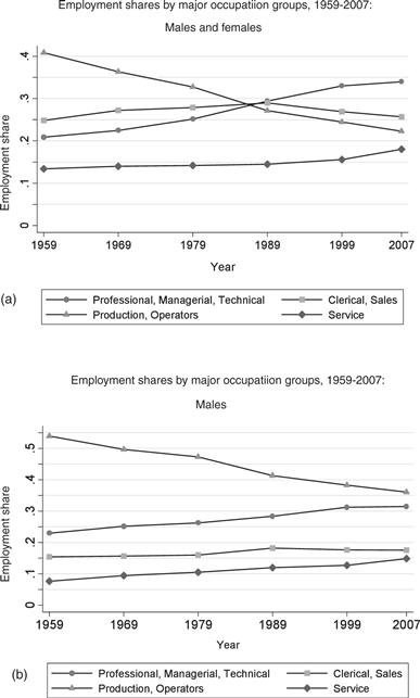
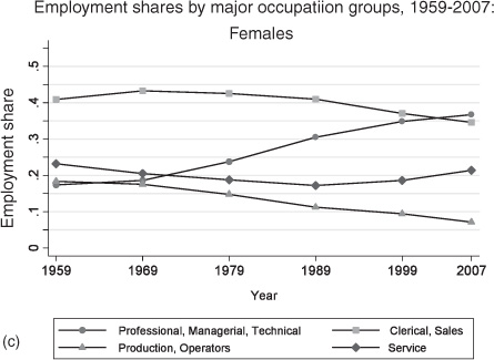
Figure 13 Source: Census IPUMS 5 percent samples for years 1960, 1970, 1980, 1990, and 2000, and Census American Community Survey for 2008. The data include all persons aged 16–64 who reported having worked last year, excluding those employed by the military and in agricultural occupations. Occupations are first assigned to 326 occupation groups that are consistent over the given time period. All non-military, non-agricultural occupations are assigned to one of four broad occupations.
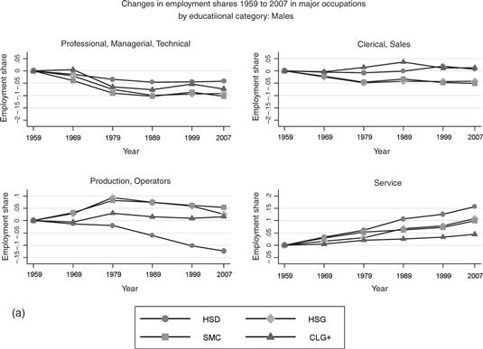
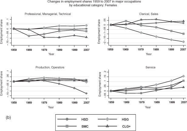
Figure 14 Source: Census IPUMS 5 percent samples for years 1960, 1970, 1980, 1990, and 2000, and Census American Community Survey for 2008. See note to Fig. 13.
This simultaneous growth of high and low-skill occupations is particularly striking in light of the substantial increases in male educational attainment in this time interval. Indeed, the fraction of employed males who had high school or lower education fell from 57 to 42 percent between 1979 and 2007, while the fraction with at least a four-year college degree rose from 20 to 28 percent.41 Simultaneously, the fraction of males at each education level employed in the highest occupational category (professional, managerial and technical occupations) declined while the fraction of males at each educational level in the lowest occupational category (service occupations) rose. Thus, the “polarization” of male employment occurs despite of rather than because of changes in male educational attainment.
Arguably, some part of the movement of high education workers into traditionally low skill jobs is arguably mechanical; as the share of workers with college education rises, it is inevitable that a subset will take traditionally non-college jobs. Nevertheless, we strongly suspect that the decline of middle skill jobs—particularly blue collar occupations—has fostered a movement of male employment in both high wage, high skill and low wage, low skill occupations. Our model below provides a formal rationale for the migration of skill groups across occupational categories in response to declining comparative advantage (e.g., due to task-replacing technologies), and makes further predictions about the extent to which these occupational movements will be primarily downward or upward.
The pattern of occupational polarization seen for males is equally evident for females. However, the net effect of declining middle skill employment on the female occupational distribution is distinct. Movement of females out of middle skill jobs is driven by a secular decline in female employment in production and operative positions (evident in every decade of our sample) and a sharp trend reversal in female employment in sales, clerical and administrative occupations—which were historically the dominant female occupational category. After hovering at 41 to 43 percent of female employment during 1959 through 1979, the share of females employed in clerical, administrative support and sales occupations fell in each of the next three decades, with a net decline of 8 percentage points.42
As with males, the slack at the middle was taken up by the tails. Female employment in professional, technical and managerial occupations rose in every decade of the sample, increasing by 6.4 percentage points between 1959 and 1979 and by another 13.0 percentage points between 1979 and 2007. However, female employment in low education service occupations rose rapidly starting in the 1990s. Between 1959 and 1989, the share of females employed in service occupations declined from 23.2 to 17.2 percent. It then rebounded. Between 1989 and 2007, female employment in service occupations rose by 4.2 percentage points (25 percent) while female employment in clerical and administrative support occupations waned.
Thus, the polarization of employment seen in aggregate in Fig. 12 is detected for both sexes, and proximately accounted for by three factors: (1) rising employment in non-routine cognitive task-intensive professional, managerial, and technical occupations; (2) rising employment in non-routine manual task-intensive service occupations; and (3) declining employment in middle skill, routine task-intensive employment in clerical, administrative support and production occupations. Although employment in middle skill jobs has fallen by considerably more among females than males between 1979 and 2007 (15.6 versus 9.6 percentage points), the offsetting employment gains have differed sharply. For females, 85 percent of the decline in middle skill jobs was offset by a rise in professional, managerial and technical occupations. For males, this share is 55 percent, with the remaining 45 percent accruing to service occupations.
These patterns of occupational change by gender and education mirror the patterns of wage changes depicted in Fig. 4. Male wage growth was sluggish or negative after 1979 for males without at least a four-year college degree. This pattern is mirrored in the downward occupational movement of non-college males seen in Fig. 14. Conversely, real wage growth for females was modestly to strongly positive for all education groups except high school dropouts after 1979. Paralleling these wage trends, female occupational composition has shifted favorably; as middle skill occupations have contracted, females with a high school degree or greater have found employment both in low skill services and in high skill professional, managerial and technical occupations.
Cross-national evidence on employment polarization
Figures 15 and 16 explore the extent to which the contemporaneous polarization of European employment, documented in Fig. 13, has stemmed from a similar set of occupational changes. Here, we use data from Eurostat to construct non-agricultural occupational employment for ten European economies for years 1992 through 2008. The eight occupational categories provided by Eurostat are coarser than the ten broad categories used above for the US in Fig. 14, and hence we further aggregate the US data for comparison. We focus on workers under age 40, since changes in occupational composition are typically first evident among workers closer to the start of their careers (Autor and Dorn, 2009).43
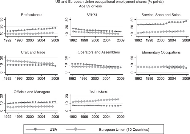
Figure 15 Source: US data from May/ORG CPS data for earnings years 1992–2009. The data include all persons aged 16–64 who reported employment in the survey reference week, excluding those employed by the military and in agricultural occupations. Occupations are first assigned to 326 occupation groups that are consistent over the given time period. From these groups, occupations are then consolidated into the eight broad categories presented in the figure. The occupation share is the percentage of all workers employed in that occupation. European data are from Eurostat data 1992–2008. The data include all persons aged 15–59 who reported having worked in the last year, excluding family workers, those employed by the military and in agricultural occupations. Occupation shares are calculated using unweighted employment data for ten European countries: Denmark, France, Germany, Greece, Ireland, Italy, the Netherlands, Portugal, Spain, and the United Kingdom.
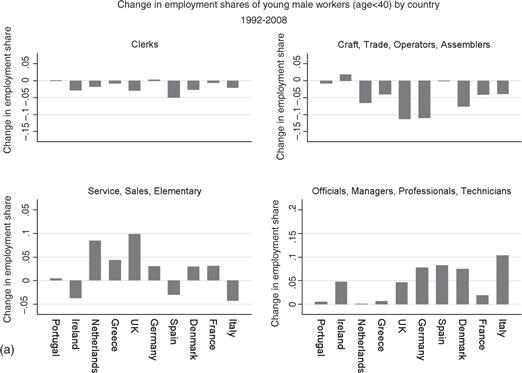
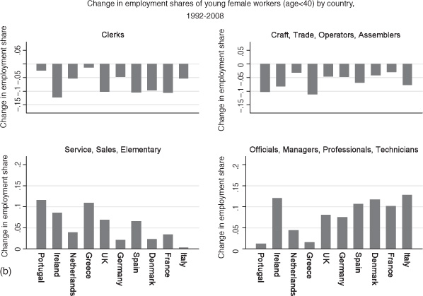
Figure 16 Source: European data from Eurostat data 1992–2008. See note to Fig. 15. Employment shares are calculated for each of the ten European countries individually, for workers under 40 years of age.
Figure 15 reveals a striking commonality in employment trends in the US and EU: high education occupations (managers, professionals, and technicians) are growing; middle education occupations (clerks, crafts and trades, and operators) and assemblers are declining; and low education service occupations (which unfortunately are aggregated with sales occupations in Eurostat) are also growing. The employment-weighted correlation of US and EU changes in employment shares by occupation is 0.63.
Since the EU averages presented in Fig. 15 potentially mask considerable crosscountry heterogeneity, we present in Fig. 16 individual changes in employment shares for all ten countries. We aggregate to the level of four occupational categories as in Figs 13 and 14, though there are some differences in aggregation required to accommodate the categories reported by Eurostat.44 In virtually every country, and for both sexes, we see a decline in clerical, craft, trade, and operative occupations—our two middle skill categories—and a rise in both professional, technical and managerial occupations and in service and elementary occupations. Indeed, for female workers, there are no exceptions to this pattern, while for males, only three countries (Portugal, Spain and Italy) show slight gains in skilled blue-collar employment or modest declines in service employment. Thus, the broad pattern of occupational change seen in the US appears to be pervasive among European economies, at least for the period in which comparable data are available (1992 through 2008).
Moving beyond these summary statistics, Goos et al. (2010) provide an in-depth analysis of occupational polarization in the EU and conclude that declines in routineintensive employment (driven by technology) are by far the largest cause. Using data on industry skill shares for the US, Japan, and nine EU economies between 1980 and 2004, Michaels et al. (2009) find that countries and industries (within countries) that differentially increased investment in information and communication technology raised their relative demand for high skill workers and reduced their relative demand for middle skill workers (whom the authors identify with routine-intensive occupations).
Is job polarization explained by industrial composition?
A more mundane explanation for employment polarization is not that “task demand” has changed per se, but rather that industry structure has shifted towards sectors that intrinsically use fewer “routine” occupations and more “abstract” and “manual” occupations. We test for this possibility with a standard shift-share decomposition of the form:
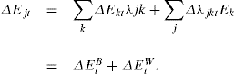 (1)
(1)
Here, Δ Ejt is the change in the overall share of employment in occupation j over time interval t, ![]() is the change in occupation j’s share of employment attributable to changes in industrial composition and, conversely,
is the change in occupation j’s share of employment attributable to changes in industrial composition and, conversely, ![]() is the change in occupation j’s employment share attributable to within-industry shifts.45 We implement this decomposition at the level of the 10 occupational categories used in Fig. 12 and an analogous division of industries into 11 consistent non-farm sectors.46
is the change in occupation j’s employment share attributable to within-industry shifts.45 We implement this decomposition at the level of the 10 occupational categories used in Fig. 12 and an analogous division of industries into 11 consistent non-farm sectors.46
Table 6 summarizes the results. In the first set of columns, we perform the decomposition separately for each of the five decades from 1959 through 2007. In the final two columns, we compare the periods 1959–1979 and 1979–2007. This latter comparison proves particularly telling.
Table 6
Decomposition of changes in the share of employment in four occupational categories by decade (percentage points) due to changes in industry shares and changes in occupational shares within industries, 1959–2007.

Source: Census IPUMS 1960, 1970,1980,1990 and 2000, and American Community Survey 2008. Each set of three rows presents the change in the share of national employment (in percentage points) in the designated occupational category and time interval and decomposes this change into between and within-industry components. The decomposition uses 10 occupation and 11 industry groups that are harmonized for the full sample interval. See text for additional details.
In both of the extended time intervals, 1959–1979 and 1979–2007, the share of employment in professional, technical and managerial occupations rose rapidly for both sexes—and particularly so for females. However, in the pre-1980 period, this rise was primarily accounted for by growth in the share of overall employment in industries that used these occupations intensively. In the latter period, three-quarters of the growth of high skill occupations reflected increased intensity of employment within rather than between industries. Similarly, the decline in clerical and sales employment was almost entirely accounted for by declining within-industry employment of workers performing these tasks. Indeed, changes in industry structure predict overall growth in clerical, administrative and sales occupations both before and after 1979. But in the latter period, these cross-industry shifts were more than offset by declining within-industry employment of these occupations—leading to net declines for these occupations.
The decline of blue-collar production and operative positions follows a pattern similar to clerical and administrative occupations, though here the pre/post 1979 contrast of between versus within-industry components is not quite as sharp. In the periods both before and after 1979, the share of employment in production, craft and operative occupations declined rapidly, averaging 3 to 5 percentage points per decade for males and 2 to 3 percentage points for females. Prior to 1980, approximately two-thirds of this decline was accounted for by shifts in industrial structure, with the rest explained by within-industry movements against blue-collar occupations. After 1979, the contraction of production, craft and operative occupations accelerated, but the source of this contraction moved from cross to within-sector shifts. Specifically, 70 percent of the decline among males and 35 percent of the decline among females was due to within-industry shifts, as compared to 40 percent and −15 percent for males and female respectively in the pre-1980 period.47
Finally, the rising share of employment in service occupations is dominated by within-industry shifts towards this occupational category. Thus, this overt manifestation of polarization is also not due to employment shifts towards service-occupation intensive sectors.
In net, this exercise indicates that shifts in industrial composition do not explain the observed polarization of employment across occupations. Within-industry shifts against middle skilled and favoring high and low skilled occupational categories are the primary driver, and the importance of these within-industry shifts is rising secularly.
It bears note that this exercise is performed at the level of fairly coarse industries, and it is possible that the between-industry component of occupational change would appear more pronounced if we were to disaggregate industries further. However, because our decomposition is currently performed at the level of 220 industry-occupation-gender cells, subdividing industries to a much finer degree would yield limited precision.48
The growing importance of occupations in wage determination
The polarization of occupational structures documented above, combined with the polarization of wage growth seen in Figs 7 through 9, jointly suggest that workers’ occupational affiliations may have become a more important determinant of wages in recent decades. Intuitively, when the evolution of earnings is monotone in educational level, education itself may be a sufficient statistic for earnings. In contrast, when employment and earnings are rising more rapidly in low and high educated occupations than in middle educated occupations, it is plausible that the explanatory power of occupations for earnings may rise.
To explore this possibility, we use Census and ACS data from 1959 through 2007 to estimate a set of cross-sectional OLS regressions of log full-time, full-year weekly wages on a quartic in potential experience and four sets of control variables (included separately): (1) years of completed schooling; (2) dummy variables for highest completed educational category (less than high school, high school graduate, some college, four-year college, post-college degree); (3) dummy variables for the 10 occupational categories used above (Table 2); and (4) dummies for the 11 industry categories used in Table 6. For each set of regressors, we calculate the partial R2 value (net of the experience quartic) in each year, and we plot these values in Fig. 17.49
Table 2
Employment and wages in ten broad occupations, 1959–2007.
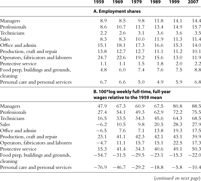
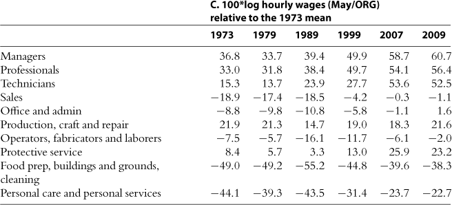
Source: Census IPUMS 5 percent samples for years 1960, 1970, 1980, 1990, and 2000, and Census American Community Survey for 2008. May/ORG CPS data for earnings years 1973–2009. Labor supply is calculated using all persons aged 1664 who reported having worked at least one week in the earnings years, excluding those in the military and agriculture. Occupations are first assigned to 326 occupation groups that are consistent over the given time period.
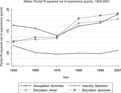
Figure 17 Source: Census IPUMS 5 percent samples for years 1960, 1970, 1980, 1990, and 2000, and Census American Community Survey for 2008. The data include all full-time, full-year workers aged 16–64, excluding those employed by the military and in agricultural occupations. Linear education measure is equal to years of educational attainment. For those who have not completed second grade, their years of education are imputed based on gender and ethnicity. Education dummies consist of five broad categories: high school dropouts, high school graduates, some college education, college graduates, and post-college degree. Occupations are assigned to 326 occupation groups that are consistent over the given time period. From these groups, occupations are then consolidated into ten broad categories: Managers; Professionals; Technicians; Sales; Office and administrative; Production, craft and repair; Operators, fabricators and laborers; Protective service; Food prep, buildings and grounds, cleaning; and Personal care and personal services. Industries are similarly converted from their respective scheme to a consistent set of 149 industries, as used in Autor et al. (1998). From these 149 industries, ten broad industry categories are constructed and include: Construction; Manufacturing; Transport and utilities; Wholesale trade; Retail trade; Finance, Insurance and Real Estate; Business services; Personal services and entertainment; Professional services; and Public administration. The partial R-squared values presented above are calculated as follows: Log weekly wages and each variable group above are orthogonalized using a quartic in experience and two ethnicity dummies. Using the residuals from each of these regressions, residual log weekly wages are regressed separately on the residuals from the variable groups of interest, and the R-squared value from this regression is plotted above for each year. All regressions are weighted byCensus person weights.
The explanatory power of educational attainment for earnings rises sharply after 1979—approximately doubling by 2007—consistent with the rising return to skill in this period. When the linear education term is replaced with a set of five education category dummies, the dummies and linear term have comparable explanatory power for the first two decades of the sample (1959–1979). After 1979, however, the explanatory power of the dummies rises substantially more (by approximately one-third) than does the linear term, reflecting the convexification of the return to education (Figs 5 and 6).50
Replacing the education measures with 10 occupation dummies produces a striking time pattern. The explanatory power of occupation reaches a nadir in 1979 and then, like the education measures, rises over the subsequent three decades. Distinct from the education measures, however, the explanatory power of the occupation variables rises less rapidly than education in the 1980s and more rapidly than education thereafter— overtaking education by 2007. Thus, as hypothesized, occupation appears to gain in importance over time. This is most pronounced starting in the 1990s, when the monotone growth of employment and earnings gives way to polarization.
One might ask whether this pattern of rising explanatory power is generally true across broad measures of job characteristics. As an alternative to occupation, we substitute the 11 industry dummies above in the wage regression. The explanatory power of industry is considerably lower than either education or occupation, and moreover has changed little over time. Thus, echoing the findings of the shift-share analysis above, occupation plays an increasingly important role in the evolution of employment and (here) earnings; it is not simply a proxy for either education or industry.
Although we have been using broad occupation categories as task proxies, it is informative to benchmark how well direct measures of job task content perform in capturing the changing wage relationships evidenced by Fig. 17. We perform this benchmark by comparing the partial R2 values of the task measures summarized in Tables 5a and 5b with both the education and occupation measures used above. To maintain equivalent coarseness of measurement, we assign task means at the level of the same 10 occupation categories using the three DOT and five O*NET task scales from Tables 5a and 5b (excluding the off shorability index). Figure 18 plots the partial R2 values.
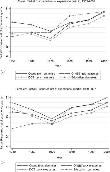
Figure 18 Source: Census IPUMS 5 percent samples for years 1960, 1970, 1980, 1990, and 2000, and Census American Community Survey for2008. See note to Fig. 17 for the partial R-squared calculation procedure. Five O*NET constructed task measures, constructed from a combination of O*NET activities and context scores, are utilized: routine cognitive, routine manual, non-routine cognitive analytic, non-routine manual, and non-routine interpersonal. Three DOT task measures are utilized, as in Autor et al. (2003): abstract, routine, and manual. See the Data Appendix for more information on the construction of the O*NET task measures.
The task measures show an even more pronounced pattern of rising explanatory power than do the occupation dummies. For males, the explanatory power of the O*NET task measures in 1979 is well below either the education or occupation dummies. But the rise in the explanatory power of the task measures is steeper than either the education or occupation measures after 1989, and it surpasses both by 2007.51 For females, the O*NET measures also exceed the education and occupation measures in explanatory power by the end of the sample, though the nadir in 1979 is not quite as low. In all cases, the DOT task measures exhibit a similar time pattern to the O*NET measures but offer somewhat lower explanatory power.
We have excluded the off shorability measure from the prior regressions because its behavior appears distinct. In Table 7, we separately investigate the explanatory power of this measure. When entered in the wage regression with the experience quartic but no other task measures, the partial R2 of the off shorability measure rises steeply for males after 1979 (from 0.026 in 1979 to 0.079 in 2007) but has no meaningful explanatory power or time trend for females after the first decade of the sample. What drives this difference by gender, we believe, is that the off shorability index is strongly monotone in education for males but non-monotone in education for females (Table 5b). As the return to education rose steeply between 1979 and 2007, the partial R2 of off shorability therefore rises for males but not for females.
Table 7
Partial R-squared values of DOT and O*NET task and off shorability measures, net of quartic in potential experience.
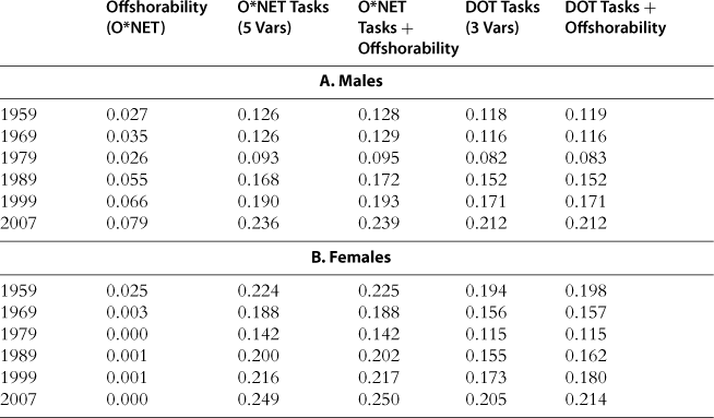
Source: O*NET, DOT and Census IPUMS 5 percent samples for years 1980, 1990, and 2000, and Census American Community Survey for 2008. See note to Fig. 17.
To assess the marginal explanatory power of the off shorability measure, Table 7 reports both the partial R2 values of the DOT and O*NET task measures entered separately and the partial R2 values of the cluster of off shorability and task measures. The off shorability measure does not add meaningfully to the explanatory power of the task measures. This result is in line with other recent work that compares the explanatory power of offshoring versus other job task measures (e.g., most importantly, routine task content) in explaining cross-region, cross-industry and cross-national trends in employment and wage polarization (Firpo et al., 2009; Michaels et al., 2009; Autor and Dorn, 2010; Goos et al., 2010). A general finding of this set of papers is that off shorability plays a comparatively small or negligible explanatory role when considered alongside other potential causes. We caution, however, that measures of both job tasks and off shorability are highly imperfect and differ substantively across studies. The conclusions drawn at this stage of the literature should therefore be viewed as provisional.52
3. The canonical model
Most economic analyses of changes in wage structure and skill differentials build on the ideas proposed in Tinbergen (1974, 1975) and developed in Welch (1973), Katz and Murphy (1992), and Card and Lemieux (2001a,b), among many others. In this approach, the college/high school log wage ratio serves as a summary index of the premium that high skill workers command relative to low skill workers, and this premium is determined by the relative supply and relative demand for skills. The relative demand for skills increases over time because changes in technology are assumed to be “skill biased,” in the sense that new technologies have greater skill demands for or are more complementary to high skill workers. Since relative supply has also steadily increased over the last century and a half, both because of the greater public investments in schooling and because of greater willingness of families and individuals to acquire schooling, this leads to Tinbergen’s famous race between technology and the supply of skills.
The effects of relative demand and supply on the earnings distribution is typically modeled in an environment with just two types of workers (high and low skill) and competitive labor markets.53 In addition, the substitution between the two types of workers is often captured using a constant elasticity of substitution aggregate production function. We refer to the framework with these features as the canonical model. In this section, we review the canonical model, explain how it provides a simple framework for interpreting several of the patterns illustrated in the previous section, and then highlight why we believe that we need to step back from or expand upon the canonical model to consider a richer framework for analyzing how the evolution of earnings and employment are shaped by the interactions among worker skills, job tasks, evolving technologies, and shifting trading opportunities.
3.1. The simple theory of the canonical model
The canonical model has two skills, high and low. It draws no distinction between skills and occupations (tasks), so that high skill workers effectively work in separate occupations (perform different tasks) from low skill workers. In many empirical applications of the canonical model, it is natural to identify high skill workers with college graduates (or in different eras, with other high education groups), and low skill workers with high school graduates (or again in different eras, with those with less than high school). We will use education and skills interchangeably, but as we discuss below, the canonical model becomes more flexible if one allows heterogeneity in skills within education groups.
Critical to the two-factor model is that high and low skill workers are imperfect substitutes in production. The elasticity of substitution between these two skill types is central to understanding how changes in relative supplies affect skill premia.
Suppose that the total supply of low skill labor is L and the total supply of high skill labor is H. Naturally not all low (or high) skill workers are alike in terms of their marketable skills. As a simple way of introducing this into the canonical model, suppose that each worker is endowed with either high or low skill, but there is a distribution across workers in terms of efficiency units of these skill types. In particular, let ![]() denote the set of low skill workers and
denote the set of low skill workers and ![]() denote the set of high skill workers. Each low skill worker i ∈
denote the set of high skill workers. Each low skill worker i ∈ ![]() has li efficiency units of low skill labor and each high skill worker i ∈
has li efficiency units of low skill labor and each high skill worker i ∈ ![]() has hi units of high skill labor. All workers supply their efficiency units inelastically. Thus the total supply of high skill and low skill labor in the economy can be written as:
has hi units of high skill labor. All workers supply their efficiency units inelastically. Thus the total supply of high skill and low skill labor in the economy can be written as:
![]()
The production function for the aggregate economy takes the following constant elasticity of substitution form
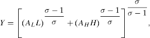 (2)
(2)
where σ e [0, ∞) is the elasticity of substitution between high skill and low skill labor, and Al and Ah are factor-augmenting technology terms.54
The elasticity of substitution between high and low skill workers plays a pivotal role in interpreting the effects of different types of technological changes in this canonical model. We refer to high and low skill workers as gross substitutes when the elasticity of substitution σ > 1, and gross complements when σ < 1. Three focal cases are: (i) σ – 0, when high skill and low skill workers will be Leontief, and output can be produced only by using high skill and low skill workers in fixed portions; (ii) σ → ∞ to when high skill and low skill workers are perfect substitutes (and thus there is only one skill, which H and L workers possess in different quantities), and (iii) σ → 1, when the production function tends to the Cobb-Douglas case.
In this framework, technologies are factor-augmenting, meaning that technological change serves to either increase the productivity of high or low skill workers (or both). This implies that there are no explicitly skill replacing technologies. Depending on the value of the elasticity of substitution, however, an increase in AH or AL can act either to complement or (effectively) substitute for high or low skill workers (see below). The lack of directly skill replacing technologies in the canonical model is an important reason why it does not necessarily provide an entirely satisfactory framework for understanding changes in the earnings and employment distributions over the last four decades.
The production function (2) admits three different interpretations.
1. There is only one good, and high skill and low skill workers are imperfect substitutes in the production of this good.
2. The production function (2) is also equivalent to an economy where consumers have utility function ![]() defined over two goods. Good Yh is produced using only high skill workers, and Yl is produced using only low skill workers, with production functions Yh = AH H, and Yl = ALL.
defined over two goods. Good Yh is produced using only high skill workers, and Yl is produced using only low skill workers, with production functions Yh = AH H, and Yl = ALL.
3. A mixture of the above two whereby different sectors produce goods that are imperfect substitutes, and high and low education workers are employed in both sectors.
Since labor markets are competitive, the low skill unit wage is simply given by the value of marginal product of low skill labor, which is obtained by differentiating (2) as
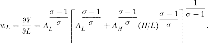 (3)
(3)
Given this unit wage, the earnings of worker i ∈ L is simply
![]()
There are two important implications of Eq. (3):
1. ∂wL/∂H/L > 0, that is, as the fraction of high skill workers in the labor force increases, the low skill wage should increase. This is an implication of imperfect substitution between high and low skill workers. An increase in the fraction (or relative supply) of high skill workers increases the demand for the services of low skill workers, pushing up their unit wage. (Formally, high and low skill workers are q-complements.)
2. ∂wL/∂AL > 0 and ∂wL/∂AH > 0, that is, either kind of factor-augmenting technical change increases wages of low skill workers (except in the limit case where σ = ∞, the second inequality is weak). This result is intuitive but will also turn out to be important: technological improvements of any sort will lead to higher wages for both skill groups in the canonical model (also following from q-complementary). Thus unless there is “technical regress,” the canonical model cannot account for declining (real) wages of a factor whose supply is not shifting outward.
Similarly, the high skill unit wage is
 (4)
(4)
We again have similar comparative statics. First, ∂wH/∂H/L < 0, so that when high skill workers become more abundant, their wages should fall. Second, ∂wH/∂AL > 0 and ∂wH/∂AH > 0, so that technological progress of any kind increases high skill (as well as low skill) wages. Also similarly, the earnings of worker i ∈ H is simply
Wi = wLhi.
It can also be verified that an increase in either AL or AH (and also an increase in H/L) will raise average wages in this model (see Acemoglu, 2002a).
Combining (3) and (4), the skill premium—the unit high skill wage divided by the unit low skill wage—is
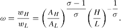 (5)
(5)
Equation (5) can be rewritten in a more convenient form by taking logs,
![]() (6)
(6)
The log skill premium, ln ω, is important in part because it is a key market outcome, reflecting the price of skills in the labor market, and it has been a central object of study in the empirical literature on the changes in the earnings distribution. Equation (6) shows that there is a simple log linear relationship between the skill premium and the relative supply of skills as measured by E/ L. Equivalently, Eq. (6) implies:
![]() (7)
(7)
This relationship corresponds to the second of the two forces in Tinbergen’s race (the first being technology, the second being the supply of skills): for a given skill bias of technology, captured here by AH/ AL, an increase in the relative supply of skills reduces the skill premium with an elasticity of 1/σ. Intuitively, an increase in H/L creates two different types of substitution. First, if high and low skill workers are producing different goods, the increase in high skill workers will raise output of the high skill intensive good, leading to a substitution towards the high skill good in consumption. This substitution hurts the relative earnings of high skill workers since it reduces the relative marginal utility of consumption, and hence the real price, of the high skill good. Second, when high and low skill workers are producing the same good but performing different functions, an increase in the number of high skill workers will necessitate a substitution of high skill workers for the functions previously performed by low skill workers.55 The downward sloping relationship between relative supply and the skill premium implies that if technology, in particular AH/ AL, had remained roughly constant over recent decades, the remarkable increase in the supply of skills shown in Fig. 1 would have led to a significant decline in the skill premium. The lack of such a decline is a key reason why economists believe that the first force in Tinbergen’s race—changes in technology increasing the demand for skills—must have also been important throughout the 20th century (cf. Goldin and Katz (2008)).
More formally, differentiating (6) with respect to AH/AL yields:
![]() (8)
(8)
Equation (8) implies that if σ > 1 , then relative improvements in the high skill augmenting technology (i.e., in AH/AL) increase the skill premium. This can be seen as a shift out of the relative demand curve for skills. The converse is obtained when σ < 1 : that is, when σ < 1, an improvement in the productivity of high skill workers, AH, relative to the productivity of low skill workers, AL, shifts the relative demand curve inward and reduces the skill premium. This case appears paradoxical at first, but is in fact quite intuitive. Consider, for example, how factor-augmenting technology change affects the wages of the augmented factor when the production function is Leontief (fixed proportions). In this case, as AH increases, high skill workers become more productive, and hence the demand for low skill workers increases by more than the demand for high skill workers. Effectively, the increase in AH creates “excess supply” of high skill workers given the number of low skill workers, which depresses the high skill relative wage. This observation raises an important caveat. It is tempting to interpret improvements in technologies used by high skill workers, AH, as “skill biased”. However, when the elasticity of substitution is less than 1 , it will be advances in technologies used with low skill workers, AL, that increase the relative productivity and wages of high skill workers, and an increase in AH relative to AL will be “skill replacing”. Nevertheless, the conventional wisdom is that the skill premium increases when high skill workers become relatively more—not relatively less—productive, which is consistent with σ > 1.56
While the case of σ < 1 is interesting (and potentially relevant when we think of different factors of production), in the context of the substitution between college and non-college workers, a relatively high elasticity of substitution is both plausible and consistent with several studies. Most estimates put σ in this context to be somewhere between 1.4 and 2 (Johnson, 1970; Freeman, 1986; Heckman et al., 1998). In this light, in what follows we assume that σ > 1.
3.2. Bringing tinbergen’s education race to the data
The key equation of the canonical model, (6), links the skill premium to the relative supply of skills, H/L, and to the relative technology term, AH / AL. This last term is not directly observed. Nevertheless, we can make considerable empirical progress by taking a specific form of Tinbergen’s hypothesis, and assuming that there is a log linear increase in the demand for skills over time coming from technology, captured in the following equation:
![]() (9)
(9)
where t is calendar time and variables written with t subscript refer to these variables at time t. Substituting this equation into (6), we obtain:
![]() (10)
(10)
Equation (10) implies that “technological developments” take place at a constant rate, while the supply of skilled workers may grow at varying rates at different points in time. Therefore, changes in the skill premium will occur when the growth rate of the supply of skills differs from the pace of technological progress. In particular, when H/L grows faster than the rate of skill biased technical change, (σ − 1) γ1, the skill premium will fall. And when the supply growth falls short of this rate, the skill premium will increase. In the next subsection, we will see that this simple equation provides considerable explanatory power for the evolution of the skill premium. At the same time, the limitations of the model become evident when it is confronted with a richer array of facts.
3.3. Changes in the US earnings distribution through the lens of the canonical model
We begin by replicating the seminal work of Katz and Murphy (1992), who demonstrated the power of the approach outlined above by fitting equation (10) to aggregate time-series data on college/high school relative wages and college/high school relative supplies for the years 1963 through 1987. Following their methods as closely as possible, the first column of Table 8 presents an OLS regression of the composition-adjusted college/high school log weekly wage premium (Fig. 1) on a linear time trend and our measure of college/high school log relative supply (Fig. 2) for years 1963–1987. We obtain the estimate:
Table 8
Regression models for the college/high school log wage gap, 1963–2008.
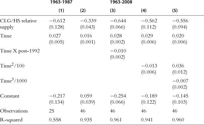
Source: March CPS data for earnings years 1963–2008. See notes to Figs 2 and 19.
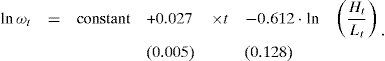
As shown in Fig. 19, this simple specification performs relatively well in capturing the broad features of the evolving college premium between 1963 and 1987, most notably, the sharp reversal of the trajectory of the college premium coinciding with the deceleration in the growth of college relative supply in the late 1970s. The power of the model is underscored in Fig. 20, which plots the college premium and college relative supply measures by year, each purged of a linear time trend. The robust inverse relationship between these two series demonstrates the key role played by the decelerating supply of college workers in driving the college premium upward in recent decades.
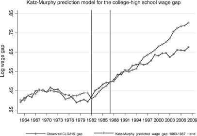
Figure 19 Source: March CPS data for earnings years 1963–2008. Log weekly wages for full-time, full-year workers are regressed separately by sex in each year on four education dummies (high school dropout, some college, college graduate, greater than college), a quartic in experience, interactions of the education dummies and experience quartic, and two race categories (black, non-white other). The composition-adjusted mean log wage is the predicted log wage evaluated for whites at the relevant experience level (5,15,25,35,45 years) and relevant education level (high school dropout, high school graduate, some college, college graduate, greater than college). The mean log wage for college and high school is the weighted average of the relevant composition adjusted cells using a fixed set of weights equal to the average employment share of each sex by experience group. The ratio of mean log wages for college and high school graduates for each year is plotted. See the Data Appendix for more details on the treatment of March CPS data. The Katz-Murphy predicted wage gap series contains the predicted values from a regression of the college/high school wage gap on time trend term and log labor supply, as measured in efficiency units described in the note to Fig. 2, for years 1963–1987.
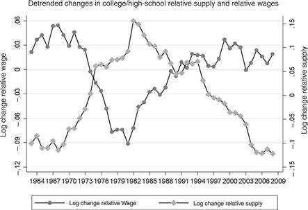
Figure 20 Source: March CPS data for earnings years 1963–2008. See note to Fig. 19. The detrended supply and wage series are the residuals from separate OLS regressions of the relative supply and relative wage measures on a constant and a linear time trend.
More formally, these estimates suggest that the evolution of the college premium during the period 1963 through 1987 can be characterized by an elasticity of substitution between college graduate workers and non-college workers of about ![]() , and an annual increase of about 2.7 percent in the relative demand for college labor.57
, and an annual increase of about 2.7 percent in the relative demand for college labor.57
Column 2 of Table 8 includes 21 additional years of data beyond 1987 to extend the Katz-Murphy estimate to 2008. When fit to this longer time period, the model yields a substantially higher estimate of the elasticity of substitution, ![]() , and a slower trend rate of demand growth (1.6 percent annually).58 The proximate cause of this change in the model’s estimated parameters can be seen in Fig. 19, which, following Autor et al. (2008), plots the out-of-sample fit of the Katz-Murphy model for the years 1987–2008. The fit of the model remains quite good through the year 1992, five years out of sample. But the model systematically deviates from the data thereafter, predicting a sharper rise in the college premium than actually occurs. While the observed college premium rose by 12 points between 1992 and 2008, the model predicts a rise of 25 log points. Without further refinements to the model, this discrepancy suggests that either the trend in relative demand decelerated after 1992 or the elasticity of substitution rose.
, and a slower trend rate of demand growth (1.6 percent annually).58 The proximate cause of this change in the model’s estimated parameters can be seen in Fig. 19, which, following Autor et al. (2008), plots the out-of-sample fit of the Katz-Murphy model for the years 1987–2008. The fit of the model remains quite good through the year 1992, five years out of sample. But the model systematically deviates from the data thereafter, predicting a sharper rise in the college premium than actually occurs. While the observed college premium rose by 12 points between 1992 and 2008, the model predicts a rise of 25 log points. Without further refinements to the model, this discrepancy suggests that either the trend in relative demand decelerated after 1992 or the elasticity of substitution rose.
Subsequent columns of Table 8 explore this possibility by freeing up the linear time trend with somewhat richer specifications: a linear spline, allowing the time trend to deviate from its initial trajectory after 1992; a quadratic time trend; and a cubic time trend. When fit to the data, all three of these variants suggest a significant deceleration in trend relative demand takes place sometime during the 1990s. Conditional on the more flexible time trend, the elasticity of substitution in these estimates returns to the range of 1.6 to 1.8. Thus, taken at face value, this model suggests that relative demand for college workers decelerated in the 1990s, which does not accord with common intuitions regarding the nature or pace of technological changes occurring in this era. We return to this point below.
One can gain additional identification and explanatory power with this model by considering a slightly richer set of facts. As shown in Tables 1a and 1b, changes in the college/high school wage gap have differed substantially by age/experience groups over recent decades. This pattern may be seen through a comparison of the college premium for younger workers (those with 0–9 years of potential experience) and older workers (those with 20–29 years of potential experience). Figure 21 shows that the rapid rise in the college/high school gap during the 1980s was concentrated among less experienced workers. Conversely, from the mid-1990s forward, the rise in the college/high school premium was greater among experienced workers.
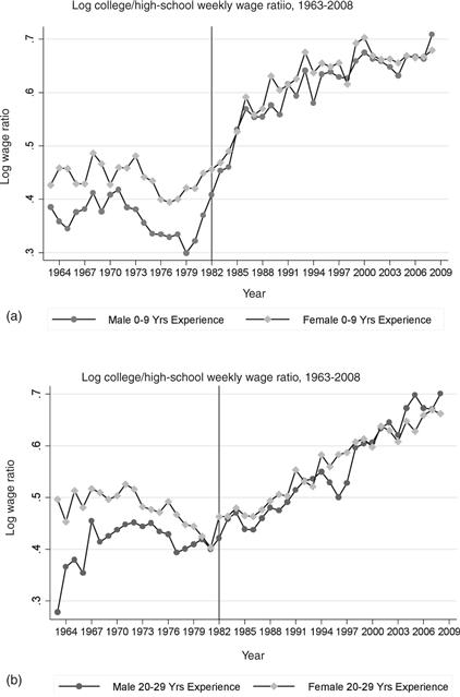
Figure 21 Source: March CPS data for earningsyears 1963–2008. See note to Fig. 19. Log college/high school weekly wage ratio for 0–9 and 20–29 years of potential experience is plotted for males and females.
These facts may better accord with a simple extension to the canonical model. To the extent that workers with similar education but different ages or experience levels are imperfect substitutes in production, one would expect age-group or cohort-specific relative skill supplies—as well as aggregate relative skill supplies—to affect the evolution of the college/high school premium by age or experience, as emphasized by Card and Lemieux (2001b). Consistent with this view, Fig. 3 (presented in Section 2) shows a rapid deceleration in relative college supply among younger workers in the mid to late 1970s, several years after the end of the Vietnam war reduced male college enrollment. Two decades later (circa 1995), this kink in the relative supply schedule generates a sharp deceleration in the availability of experienced college workers. Notably, the differential rises in the college premium for young and (later) for experienced workers roughly coincide with the differential slowdown in college supply among these experience groups (though these slowdowns are 20 years apart). This pattern offers a prima facie case that the college premium for an experience group depends on its own-group relative supply as well as the overall supply of college relative to high school graduates.
We take fuller account of these differing trends by experience group in Table 9 by estimating regression models for the college wage by experience group. These extend the basic specification in Eq. (10) to include own experience group relative skill supplies. The first column of Table 10 presents a regression pooled across 4 potential experience groups (those with 0–9, 10–19, 20–29, and 30–39 years of experience), allowing for group-specific intercepts but constraining the other coefficients to be the same for all experience groups. Specifically, we estimate:
Table 9
Regression models for the college/high school log wage gap by potential experience group, 1963–2008.
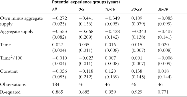
Source: March CPS data for earnings years 1963–2008. See notes to Figs 2 and 19.
Table 10
OLS stacked first-difference estimates of the relationship between demographic group occupational distributions in 1959 and subsequent changes in demographic groups’ mean log wages by decade, 1959–2007.
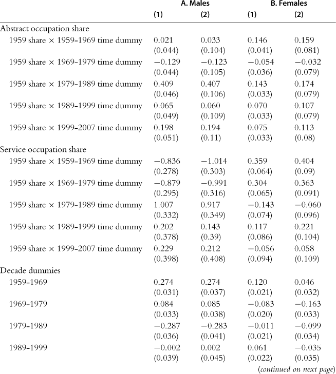
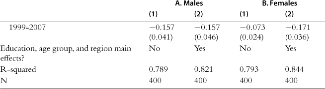
Source: Census IPUMS 1960,1970, 1980, 1990 and 2000, and American Community Survey 2008. Each column presents a separate OLS regression of stacked changes in mean log real hourly wages by demographic group and year, where demographic groups are defined by sex, education group (high school dropout, high school graduate, some college, college degree, post-college degree), age group (25–34, 35–44, 45–54, 55–64), and region of residence (Northeast, South, Midwest, West). Models are weighted by the mean start and end-year share of employment of each demographic group for each decadal change. Occupation shares are calculated for each demographic group in 1959 (using the 1960 Census) and interacted with decade dummies. Occupations are grouped into three exhaustive and mutually exclusive categories: (1) abstract—professional, managerial and technical occupations; (2) service—protective service, food service and cleaning, and personal services occupations; (3) routine—clerical, sales, administrative support, production, operative and laborer occupations. The routine group is the omitted category in the regression models.
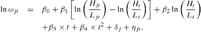
where j indexes experience groups, δj is a set of experience group main effects, and we include a quadratic time trend. This specification arises from an aggregate constant elasticity of substitution production function in which college and high school equivalents from the aggregate inputs, similar to Eq. (2) above, where these aggregate inputs are themselves constant elasticity of substitution sub-aggregates of college and high school labor by experience group (Card and Lemieux, 2001b). Under these assumptions, 1 /β1 provides an estimate of σ2, the aggregate elasticity of substitution, and 1 /β provides an estimate of σj, the partial elasticity of substitution between different experience groups within the same education group.
The estimates in the first column of Table 9 indicate a substantial effect of both own-group and aggregate supplies on the evolution of the college wage premium by experience group. While the implied estimate of the aggregate elasticity of substitution in this model is similar to the aggregate models in Table 8, the implied value of the partial elasticity of substitution between experience groups is around 3.7 (which is somewhat smaller than the estimates in Card and Lemieux (2001b)). This model indicates that differences in own-group relative college supply go some distance towards explaining variation across experience groups in the evolution of the college wage premium in recent decades.
The final four columns of Table 9 present regression models of the college wage premium estimated separately by experience group. These estimates show that trend demand changes and relative skill supplies play a large role in changes in educational differentials for younger and prime age workers. The college wage premium for workers with under 20 years of experience is quite responsive to both own group and aggregate relative skill supplies. However, aggregate supplies appear equally important for workers with 20-plus years of experience, while own-group supplies are not found to exert an independent effect.
3.4. Overall inequality in the canonical model
Our brief overview of the salient empirical patterns in the previous section highlights that there have been rich and complex changes in the overall earning distribution over the last four decades. While changes in the college premium (or more generally in the returns to different levels of schooling) have contributed to these changes in the earnings distribution, there have also been significant changes in inequality among workers with the same education—i.e., within groups as well as between groups.
The canonical model introduced above can also provide a first set of insights for thinking about within-group inequality and thus provides a framework for interpreting changes in the overall wage distribution. In particular, the model generates not only differing wages for high and low skill workers, but also wage variation among workers with a given level of observed skill. This follows from our assumption that the efficiency units of labor supplies vary across workers of each skill group.
Nevertheless, this type of within group inequality (i.e., due to cross-worker, within skill group heterogeneity in efficiency units) is invariant to skill prices and thus changes in overall inequality in this model will closely mimic changes in the skill premium. In particular, recall that all workers in the set L (respectively in the set H) always face the same skill price. Therefore changes in the skill premium should have no direct effect on within group inequality. Mathematically, in this model the relative earnings of two workers in the same group, say L, is given by
![]()
In this simple form, the canonical model can exhibit significant within group wage inequality, but inequality will be independent of the skill premium.59
Naturally, this feature can be changed by positing that there are increasing returns to efficiency units of skill, so when the relative demand for high skill labor increases, this increases the demand for “more skilled” college graduates by relatively more than for “less skilled” college graduates. One way to incorporate this idea is to extend the canonical model by drawing a distinction between observable groups (such as college vs. non-college) and skills. For example, we can remain fairly close to the spirit of the canonical model and continue to assume that there are only two skills, but now suppose that these skills are only imperfectly approximated by education (or experience).
Specifically, we can assume that the two observable groups are college and non-college, and a fraction φc of college graduates are high skill, while a fraction ϕn < ϕc of non-college graduates are high skill (the remaining fractions in both groups being low skill as usual). Let us again denote the skill premium by ω = wH/wL. This is no longer the college premium, i.e., the ratio of average college to non-college wages, however, since not all college workers have high skill and not all non-college workers have low skill. Given our assumption, we can compute the college premium simply as the ratio of (average) college wages, wC, to (average) non-college wages, wN, that is,
![]()
It is straightforward to verify that, because ϕn < ϕc, this college premium is increasing in ω, so that when the true price of skill increases, the observed college premium will also rise. In addition, we can define within group inequality in this context as the ratio of the earnings of high wage college graduates (or non-college graduates) to that of low wage college graduates (or non-college graduates). Given our assumptions, we also have ωwithin = ω (since high wage workers in both groups earn wH, while low wage workers earn wL). As long as ϕc and ϕn remain constant, ωc and ωwithin will move together. Therefore in this extended version of the canonical model, an increase in the returns to observed skills—such as education—will also be associated with an increase in the returns to unobserved skills. Moreover, we can also think of large changes in relative supplies being associated with compositional changes, affecting ϕc and ϕη, so within group inequality can change differently than the skill premium, and thus overall inequality can exhibit more complex changes as supplies and technology evolve.60
This model thus provides a useful starting point for thinking about changes in within group inequality and the overall earnings distribution, and linking them both to the market price of skills. In light of this model, the increase in the overall earnings inequality starting in the late 1970s or early 1980s is intimately linked to the increase in the demand for skills, also reflected in the increase in the college premium. While this parsimonious framework is valuable for analyzing the evolution of distribution of earnings, it does not provide sufficient nuance for understanding why different parts of the earnings distribution move differently and, moreover, do so markedly during different time periods.
3.5. Endogenous changes in technology
The canonical model is most powerful as an empirical framework when skill biased technical change can be approximated by a steady process, such as the (log) linear trend posited in (9). However, the discussion in Autor et al. (1998) suggests that the pace of skill biased technical change was likely more rapid between 1970 and 1990 than between 1940 and 1970. The evidence discussed above, on the other hand, suggests that the pace of skill biased technical change slowed during the 1990s, at least viewed through the lens of the canonical model. As also discussed in Acemoglu (2002a), a relatively steady process of skill biased technical change is likely to be a particularly poor approximation when we consider the last 200 years instead of just the postwar period. For example, the available evidence suggests that the most important innovations of the nineteenth century may have replaced—rather than complemented—skilled workers (in particular artisans). The artisanal shop was replaced by the factory and later by interchangeable parts and the assembly line, and products previously manufactured by skilled artisans were subsequently produced in factories by workers with relatively few skills (see, e.g., Mokyr, 1992; James and Skinner, 1985; Goldin and Katz, 2008; Hounshell, 1985; Acemoglu, 2002a).
But once we recognize that skill biased technical change is not a steady process, it becomes more important to understand when we should expect it to be more rapid (and when we should expect it not to take place at all). The canonical model is silent on this question. Acemoglu (1998, 2002a) suggests that modeling the endogenous response of the skill bias of technology might generate richer insights. In particular, as we discuss further in Section 4.8, under relatively general conditions, models of endogenous (directed) technical change imply that technology should become more skill biased following increases in the supply of high skill workers (and conversely, less skill biased following increases in the supply of low skill workers). According to this perspective, steady skill biased technical change might be partly a response to the steady increase in the supply of skills during the past century (thus uniting the two parts of Tinbergen’s race); the skill replacing technologies of the nineteenth century might be partly a response to the large increase in the supply of low skill workers in the cities; the acceleration in skill bias in the 1980s might, in part, be a response to the more rapid increase in the supply of college skills in the late 1960s and early 1970s noted in Section 2; and the deceleration of demand shifts favoring skilled workers in the 1990s might in part be a response to the deceleration in the supply of college skills during the 1980s (see again Section 2).
As we discussed above, computer technology is particularly well suited for automating routine tasks. This creates a natural tendency for the type of skill bias described by Autor et al. (2003). It does not, however, imply that the path of technical change and its bias are entirely exogenous. Exactly how computer technology is developed and how it is applied in the production process has much flexibility, and it is plausible that this will respond to profit opportunities created by different types of applications and uses.