
Chapter 9
The Role of Vibronic Coupling for Intersystem Crossing and Reverse Intersystem Crossing Rates in TADF Molecules
Thomas J. Penfold and Jamie Gibson
Newcastle University, School of Chemistry, NE1 7RU Newcastle upon Tyne, UK
9.1 Introduction
Since the first report of electroluminescence (EL) in poly(para‐phenylenevinylene) [1], there has been an enormous amount of effort dedicated to the development of organic light‐emitting diodes (OLEDs). However, early attempts to implement OLEDs based solely upon organic materials were restricted by an intrinsically low EL efficiency. This arose from the limit imposed by the statistics of the spin states formed under electrical excitation. Indeed, following electrical excitation only 25% of the excitons exist in the singlet states, while the remaining 75% form triplet excitons [2]. For organic species the latter, the triplet states, are not (strongly) dipole coupled to the molecular ground state due to the absence of strong spin–orbit coupling (SOC). Consequently, this energy cannot be harvested and is dissipated nonradiatively.
This limitation was overcome by doping the emitting layer with metal–organic emitters [3] yielding the so‐called phosphorescence‐based organic light‐emitting diodes (PhOLEDs). For these devices, the presence of a metal–organic complex containing heavy atoms opens the potential for significant SOC and gives rise to a radiative T![]() S
S![]() transition (triplet harvesting) [4]. The radiative rate of this transition,
transition (triplet harvesting) [4]. The radiative rate of this transition, ![]() , crucial to device efficiency [5] is formally zero but gains intensity through spin–orbit mixing with the close‐lying singlet states S
, crucial to device efficiency [5] is formally zero but gains intensity through spin–orbit mixing with the close‐lying singlet states S![]() :
:

where ![]() is the transition dipole moment between the ground state (S
is the transition dipole moment between the ground state (S![]() ) and excited singlet states, S
) and excited singlet states, S![]() .
. ![]() describes the first‐order mixing coefficient between triplet states (T
describes the first‐order mixing coefficient between triplet states (T![]() ) that besides stimulating
) that besides stimulating ![]() also promotes intersystem crossing (ISC) and reverse intersystem crossing (rISC). The second sum in the brackets describes the contribution to the phosphorescence rate owing to the perturbation of the electronic ground state, i.e. singlet ground state gaining triplet character, in contrast to triplet excited states mixing with singlet states. It is often argued that the energy gap between the electronic ground state and the excited triplet states is so much larger than the energy difference between the T
also promotes intersystem crossing (ISC) and reverse intersystem crossing (rISC). The second sum in the brackets describes the contribution to the phosphorescence rate owing to the perturbation of the electronic ground state, i.e. singlet ground state gaining triplet character, in contrast to triplet excited states mixing with singlet states. It is often argued that the energy gap between the electronic ground state and the excited triplet states is so much larger than the energy difference between the T![]() state and the excited singlet states and that the second sum can be neglected. However, this disregards the fact that the sum over
state and the excited singlet states and that the second sum can be neglected. However, this disregards the fact that the sum over ![]() includes
includes ![]() , i.e. the electronic ground state, and that the term for
, i.e. the electronic ground state, and that the term for ![]() in the second perturbation sum partially cancels this contribution. To avoid artefacts in the calculation, both perturbation sums should be always considered.
in the second perturbation sum partially cancels this contribution. To avoid artefacts in the calculation, both perturbation sums should be always considered.
However, although this approach can be extremely effective, until now the only phosphorescent materials found practically useful are iridium and platinum complexes, which are unappealing for commercial applications due to their high cost and low abundance [6]. Indeed, as iridium is the fourth most scarce naturally occurring element on the planet, it is unwise to base such large‐scale technologies such as lighting and displays on it.
An exciting new avenue for effective harvesting of both the singlet and triplet excitons can be achieved by using materials that emit through thermally activated delayed fluorescence (TADF) [7]. Here, the triplet excitons (75%) are not emitted through the T![]() radiative transition, but use thermal energy to promote upconversion via rISC so that they can emit as singlet excitons. This means that effective TADF requires the emitters to have both a small energy gap
radiative transition, but use thermal energy to promote upconversion via rISC so that they can emit as singlet excitons. This means that effective TADF requires the emitters to have both a small energy gap ![]() E
E![]() between the emitting singlet and triplet states, preferably
between the emitting singlet and triplet states, preferably ![]() 0.1 eV, and a nonzero SOC that mixes their spin character and permits efficient rISC, as shown in Eq. (9.1). The size of the former (
0.1 eV, and a nonzero SOC that mixes their spin character and permits efficient rISC, as shown in Eq. (9.1). The size of the former (![]() E
E![]() ) is two times the electron exchange interaction (2
) is two times the electron exchange interaction (2![]() ) between the ground and excited states [8]:
) between the ground and excited states [8]:

where ![]() and
and ![]() represent ground‐ and excited‐state wave functions, respectively;
represent ground‐ and excited‐state wave functions, respectively; ![]() is the charge; and
is the charge; and ![]() is the dielectric constant. This can usually be well approximated using the spatial overlap between the highest occupied molecular orbital (HOMO) and lowest unoccupied molecular orbital (LUMO), and consequently, the most promising TADF emitters have exploited charge‐transfer (CT) states that minimize the spatial overlap and therefore the exchange energy [9], [10]. Crucially, as shown in Eq. (9.1), this small energy gap is able to promote significant mixing between the singlet and triplet states, which depends inversely on the energy gap provided SOC is nonzero. This relationship reduces the emphasis upon the magnitude of SOC and opens the possibility for devices that contain exclusively organic materials [11], [12]. The challenge of this approach is that reducing the spatial overlap between the HOMO and LUMO orbitals also reduces the radiative rate of the emitting S
is the dielectric constant. This can usually be well approximated using the spatial overlap between the highest occupied molecular orbital (HOMO) and lowest unoccupied molecular orbital (LUMO), and consequently, the most promising TADF emitters have exploited charge‐transfer (CT) states that minimize the spatial overlap and therefore the exchange energy [9], [10]. Crucially, as shown in Eq. (9.1), this small energy gap is able to promote significant mixing between the singlet and triplet states, which depends inversely on the energy gap provided SOC is nonzero. This relationship reduces the emphasis upon the magnitude of SOC and opens the possibility for devices that contain exclusively organic materials [11], [12]. The challenge of this approach is that reducing the spatial overlap between the HOMO and LUMO orbitals also reduces the radiative rate of the emitting S![]() state. While high fluorescence efficiencies are important for high performing devices, it is more important that the radiative decay rate is much faster than all nonradiative rates (
state. While high fluorescence efficiencies are important for high performing devices, it is more important that the radiative decay rate is much faster than all nonradiative rates (![]() ), and therefore during the design of TADF emitters, it is important to understand the processes contributing to
), and therefore during the design of TADF emitters, it is important to understand the processes contributing to ![]() and reduce them as much as possible.
and reduce them as much as possible.
As illustrated in the previous paragraph, for third‐generation TADF OLED devices, the communication between low‐lying singlet and triplet excited states is of great importance and plays a fundamental role in determining key molecular and material properties relevant in a device context. Consequently, a thorough understanding of the basic principles governing the interplay between these manifolds of spin states is of great importance if one is to achieve systematic material design. Computationally, the most common approach for elucidating mechanistic information about processes occurring in electronically excited states is to compute energy profiles along viable reaction and/or decay pathways. These are usually represented as one‐dimensional curves, ![]() in Figure 9.1, containing displacements along multiple nuclear degrees of freedom. Important regions of the potential surface, such as crossings between states of the same or different multiplicities, potentially contributing to internal conversion (IC) and ISC, respectively (Figure 9.1), can also be identified. While useful, the resulting picture is static and lacks the dynamical information important for obtaining a complete understanding, especially given the complexity that can arise from dynamics occurring on a multidimensional potential energy surface (PES). This is especially pertinent in cases that exhibit a breakdown of the Born–Oppenheimer approximation, giving rise to nonadiabatic coupling [13]. Indeed, these nonadiabatic interactions arise from nuclear motion and occur via a dynamic effect in the sense that they become strong when a system traverses a region where coupled states are close in energy or degenerate, leading to a more efficient crossing. In this chapter an overview of dynamical methods used for understanding excited‐state processes is provided. We then summarize our recent research using quantum nuclear dynamics to understand the role of vibronic coupling for ISC and rISC rates in two molecules with implications to TADF.
in Figure 9.1, containing displacements along multiple nuclear degrees of freedom. Important regions of the potential surface, such as crossings between states of the same or different multiplicities, potentially contributing to internal conversion (IC) and ISC, respectively (Figure 9.1), can also be identified. While useful, the resulting picture is static and lacks the dynamical information important for obtaining a complete understanding, especially given the complexity that can arise from dynamics occurring on a multidimensional potential energy surface (PES). This is especially pertinent in cases that exhibit a breakdown of the Born–Oppenheimer approximation, giving rise to nonadiabatic coupling [13]. Indeed, these nonadiabatic interactions arise from nuclear motion and occur via a dynamic effect in the sense that they become strong when a system traverses a region where coupled states are close in energy or degenerate, leading to a more efficient crossing. In this chapter an overview of dynamical methods used for understanding excited‐state processes is provided. We then summarize our recent research using quantum nuclear dynamics to understand the role of vibronic coupling for ISC and rISC rates in two molecules with implications to TADF.

Figure 9.1A schematic representation of the adiabatic electronic energies against an arbitrary nuclear configuration  . Coupling between states of the same multiplicity originating from nonadiabatic coupling gives rise to internal conversion (IC). Transitions between states of different multiplicities, intersystem crossing (ISC), arise from spin–orbit coupling.
9.1.1 Background to Delayed Fluorescence
Molecular fluorescence is usually a two‐step process, i.e. an initial absorption giving rise to an electronically excited state followed by the radiative decay of that state or another one of lower energy (Kasha's rule) into the electronic ground state. This is known as prompt fluorescence (PF). However, if the florescence and nonradiative decay rate from this state is a lot less than the rate of ISC, i.e. ![]() (see Figure 9.2), then fluorescence may occur by a more complicated route, the triplet manifold. In this case, the S
(see Figure 9.2), then fluorescence may occur by a more complicated route, the triplet manifold. In this case, the S![]() state decays via ISC into the T
state decays via ISC into the T![]() state. Subsequently, if the phosphorescence and nonradiative decay of the triplet state is slow, as expected, and the energy gap between the singlet and triplet states is small enough (normally
state. Subsequently, if the phosphorescence and nonradiative decay of the triplet state is slow, as expected, and the energy gap between the singlet and triplet states is small enough (normally ![]() 0.2 eV), then after vibrational thermalization, a second ISC, often called rISC, back to the S
0.2 eV), then after vibrational thermalization, a second ISC, often called rISC, back to the S![]() can occur followed by emission. This is known as delayed fluorescence (DF). If all radiative and nonradiative processes are very small, this process can occur multiple times before DF actually occurs. The system can therefore be said to be cycling between the two states [15].
can occur followed by emission. This is known as delayed fluorescence (DF). If all radiative and nonradiative processes are very small, this process can occur multiple times before DF actually occurs. The system can therefore be said to be cycling between the two states [15].

Figure 9.2 A simplified energy diagram representing a general schematic of the upconversion of triplet states to a higher‐energy singlet state.  is approximately equal to the
  multiplied by a Boltzmann term, which determines the number of states with sufficient energy to overcome the barrier (
 ). Deviations from this relationship arise from a higher density of final states expected for the direct intersystem crossing case.
Source: Ref. [14]. Reproduced with permission of American Chemical Society.
The first observation of DF was by Perrin and coworkers [16] who reported two long‐lived emission bands in solid uranyl salts naming them true phosphorescence and fluorescence of long duration. This was later characterized in more detail by Lewis et al. [17] in rigid media and Parker and Hatchard [18] using Eosin. The latter study is responsible for the original name, E‐type DF, which is now most commonly referred to as TADF.
The most common description of TADF is the equilibrium model, first proposed by Parker and Hatchard [18] and later used by Kirchhoff et al. [19] to describe the TADF of Cu(I) metal–organic complexes. This assumes that ![]() , and in this limit the steady‐state populations of the emitting singlet and triplet states are determined by Boltzmann statistics, as the molecule spends sufficient time in the excited state for an equilibrium to form before emission eventually occurs. The relative population of the two states can be expressed using an equilibrium constant:
, and in this limit the steady‐state populations of the emitting singlet and triplet states are determined by Boltzmann statistics, as the molecule spends sufficient time in the excited state for an equilibrium to form before emission eventually occurs. The relative population of the two states can be expressed using an equilibrium constant:

making it possible to express the rate of the whole TADF process (![]() ), i.e. rISC proceeded by fluorescence as the product of the amount of population in the S
), i.e. rISC proceeded by fluorescence as the product of the amount of population in the S![]() state and the rate‐limiting step, i.e.
state and the rate‐limiting step, i.e. ![]() :
:
Here, the prefactor of ![]() is a consequence of the three triplet substates (i.e.
is a consequence of the three triplet substates (i.e. ![]() ). This approach, adopted by Adachi and coworkers [12], [20] for organic emitters, defines the TADF process as depending exclusively on the energy gap between the singlet and triplet states and crucially, as shown in Eq. (9.4), independent of the coupling between them, i.e. the rates of ISC (
). This approach, adopted by Adachi and coworkers [12], [20] for organic emitters, defines the TADF process as depending exclusively on the energy gap between the singlet and triplet states and crucially, as shown in Eq. (9.4), independent of the coupling between them, i.e. the rates of ISC (![]() ) and rISC (
) and rISC (![]() ), provided they are not zero. This motives design procedures that focus upon minimizing this energy gap using CT states and suppressing larger amplitude molecular vibrations to reduce nonradiative pathways to ensure a maximum emission quantum yield, despite the potentially low radiative rates associated with the CT states.
), provided they are not zero. This motives design procedures that focus upon minimizing this energy gap using CT states and suppressing larger amplitude molecular vibrations to reduce nonradiative pathways to ensure a maximum emission quantum yield, despite the potentially low radiative rates associated with the CT states.
While this represents a convenient approach for the analysis of photophysical data, the key assumption, i.e. ![]() , must be and often is broken to support new emitters with stronger fluorescence yields [20], [21]. Within this regime, TADF is cast in terms of a kinetic process [22], for which the population of the emitting states in the longtime limit, assuming nonradiative and phosphorescence channels are small, can be expressed as
, must be and often is broken to support new emitters with stronger fluorescence yields [20], [21]. Within this regime, TADF is cast in terms of a kinetic process [22], for which the population of the emitting states in the longtime limit, assuming nonradiative and phosphorescence channels are small, can be expressed as


Solving Eqs. (9.5a) and (9.5b) yields

This illustrates the importance in not only tuning the energy gap, as is the focus from the equilibrium representations presented in Eq. (9.4), but also determining and optimizing other factors that influence ![]() , for which a wide variety of values exist in the literature. This was recently affirmed by Inoue et al. [23] who demonstrated significant reduction in device roll‐off efficiency for complexes exhibiting larger
, for which a wide variety of values exist in the literature. This was recently affirmed by Inoue et al. [23] who demonstrated significant reduction in device roll‐off efficiency for complexes exhibiting larger ![]() , as the device is less susceptible the quenching effects, such as triplet–triplet annihilation.
, as the device is less susceptible the quenching effects, such as triplet–triplet annihilation.
9.1.2 The Mechanism of rISC
In Section 9.1.1 the core elements of TADF and the importance of ![]() were established. However, despite the significant amount of research undertaken in this area, the mechanism for rISC and especially the efficient rISC recently reported in organic emitters (
were established. However, despite the significant amount of research undertaken in this area, the mechanism for rISC and especially the efficient rISC recently reported in organic emitters (![]() s
s![]() [20], [21]) has not been fully established.
[20], [21]) has not been fully established.
Transitions between two states of different spin multiplicities usually occur via the SOC interaction [24]. SOC between the lowest singlet and triplet metal–ligand CT states (![]() MLCT and
MLCT and ![]() MLCT) of Cu(I) complexes [25] is small but usually sufficient to explain the values of
MLCT) of Cu(I) complexes [25] is small but usually sufficient to explain the values of ![]() and
and ![]() reported [26]. For Cu(I) complexes that exhibit significant conformation freedom within the excited states, it can be important to also consider the SOC beyond the Franck–Condon geometry and incorporate how vibrational motion affects its magnitude, i.e. spin–vibronic coupling; see Refs. [27]–[32]. However, the situation is not quite so simple for donor–acceptor (D–A) complexes, which form the majority of organic TADF emitters. Indeed, Lim et al. [33] showed that SOC between
reported [26]. For Cu(I) complexes that exhibit significant conformation freedom within the excited states, it can be important to also consider the SOC beyond the Franck–Condon geometry and incorporate how vibrational motion affects its magnitude, i.e. spin–vibronic coupling; see Refs. [27]–[32]. However, the situation is not quite so simple for donor–acceptor (D–A) complexes, which form the majority of organic TADF emitters. Indeed, Lim et al. [33] showed that SOC between ![]() CT and
CT and ![]() CT in these intramolecular charge transfer (ICT) complexes is formally zero. This is because spin–orbit coupling matrix elements (SOCMEs) between a singlet and triplet state with equal spatial orbital occupations are formally forbidden. The origin of this is analogous to El‐Sayed's law [34] regarding conservation of total angular momentum during spin–flip transitions.
CT in these intramolecular charge transfer (ICT) complexes is formally zero. This is because spin–orbit coupling matrix elements (SOCMEs) between a singlet and triplet state with equal spatial orbital occupations are formally forbidden. The origin of this is analogous to El‐Sayed's law [34] regarding conservation of total angular momentum during spin–flip transitions.
This issue, limiting our understanding of the mechanisms driving rISC, would appear reduced by the observation that the lowest triplet state for many complexes exhibiting efficient rISC is a ![]() locally excited triplet state (
locally excited triplet state (![]() LE) [21], [35]. In this case
LE) [21], [35]. In this case ![]() LE
LE ![]() CT conversion could have a finite, if small, SOCME permitting rISC. However, using a Fermi's golden rule (FGR) approach, Chen et al. [36] showed that the rate of
CT conversion could have a finite, if small, SOCME permitting rISC. However, using a Fermi's golden rule (FGR) approach, Chen et al. [36] showed that the rate of ![]() LE
LE ![]() CT conversion in a series of TADF molecules was
CT conversion in a series of TADF molecules was ![]() s
s![]() , four to five orders of magnitude less than the rates reported experimentally, and consequently a key component leading to complete understanding is clearly lacking.
, four to five orders of magnitude less than the rates reported experimentally, and consequently a key component leading to complete understanding is clearly lacking.
To address this, Ogiwara et al. [37] used electron paramagnetic resonance (EPR) spectroscopy to probe the population of the ![]() LE and
LE and ![]() CT states. By fitting the transient experimental signals, they reported that complexes showing the largest rISC exhibited an EPR signal consistent with a mixture of both the
CT states. By fitting the transient experimental signals, they reported that complexes showing the largest rISC exhibited an EPR signal consistent with a mixture of both the ![]() LE and
LE and ![]() CT states. The authors used this to propose that efficient rISC includes not only the SOC pathway (
CT states. The authors used this to propose that efficient rISC includes not only the SOC pathway (![]() LE
LE ![]() CT) but also a hyperfine coupling‐induced ISC pathway (
CT) but also a hyperfine coupling‐induced ISC pathway (![]() CT
CT ![]() CT). This mechanism arises from interactions between an electron's spin and the magnetic nuclei of its molecule. It is therefore completely local and not quenched by significant electron‐hole separation experienced in CT states like SOC [38]. This conclusion is consistent with the proposal of Adachi and coworkers [20], who rationalized efficient rISC from
CT). This mechanism arises from interactions between an electron's spin and the magnetic nuclei of its molecule. It is therefore completely local and not quenched by significant electron‐hole separation experienced in CT states like SOC [38]. This conclusion is consistent with the proposal of Adachi and coworkers [20], who rationalized efficient rISC from ![]() LE to
LE to ![]() CT, as proceeding via reverse internal conversion (rIC) to the
CT, as proceeding via reverse internal conversion (rIC) to the ![]() CT and then using hyperfine coupling‐induced ISC to cross to the
CT and then using hyperfine coupling‐induced ISC to cross to the ![]() CT. However, crucially the hyperfine coupling constants are very small, usually in the range of 10
CT. However, crucially the hyperfine coupling constants are very small, usually in the range of 10![]() meV, and they therefore also appear highly unlikely that such coupling accounts for efficient rISC.
meV, and they therefore also appear highly unlikely that such coupling accounts for efficient rISC.
Recently D–A and D–A–D complexes reported by Ward et al. [39] point to a strong dynamical component to the rISC mechanism. Indeed, their work found that complexes including steric hindrance around the D–A dihedral angle switch off the main TADF pathway and make the molecule phosphorescent at room temperature. This dynamical aspect, i.e. motion along the D–A dihedral coordination, which appears to promote rISC is consistent with the recent simulations of Marian [40] who used multireference quantum chemistry methods to show, in agreement with Ref. [36], that direct SOC was indeed too small to explain efficient rISC. Marian proposed that it is mediated by mixing with an energetically close‐lying ![]() LE state along a carbonyl stretching mode, promoting spin–vibronic mixing between multiple excited states as being crucial to efficient rISC. Similar mechanisms have been widely reported for the ISC rate [27]–[32]. However while hugely informative, these calculations are inherently static and therefore do not provide mechanistic understanding of the TADF process. For this detail, simulations with temporal resolution are required and are the focus of the present work.
LE state along a carbonyl stretching mode, promoting spin–vibronic mixing between multiple excited states as being crucial to efficient rISC. Similar mechanisms have been widely reported for the ISC rate [27]–[32]. However while hugely informative, these calculations are inherently static and therefore do not provide mechanistic understanding of the TADF process. For this detail, simulations with temporal resolution are required and are the focus of the present work.
9.2 Beyond a Static Description
The rate of population transfer between two states can be described using a FGR approach as described in Ref. [28]. This was illustrated using high‐level quantum chemistry calculations of the rISC rates for both Cu(I) and organic TADF molecules. This first‐order perturbative approach is very effective, as demonstrated on numerous occasions by Marian and coworkers [27]–[29], describing the excited‐state kinetics, provided that the coupling between the two states is small compared with their energy difference. If this is not the case, the validity of this approach, i.e. perturbation theory, becomes questionable, although it has still been used with some success [41].
Importantly, as described in the previous section, recent work demonstrates a dynamical mechanism for efficient rISC [39], [42]. This strongly motivates computations that go beyond inherently static quantum chemistry calculations and solves the time‐dependent motion of the nuclei over a PES to elucidate a full understanding of the fine mechanistic details. In the following subsections we describe a variety of approaches for achieving this.
The starting point for any attempts aiming to elucidate fine details about excited‐state dynamics is the time‐dependent Schrödinger equation (TDSE):
To derive working equations from this, the Born–Huang ansatz [43] for the total wave function is applied:

where ![]() describes a complete set of electronic states that are solutions of the time‐independent electronic Schrödinger equation:
describes a complete set of electronic states that are solutions of the time‐independent electronic Schrödinger equation:
In practice solutions for ![]() are achieved using a quantum chemistry method at various configurations in nuclear coordinate space,
are achieved using a quantum chemistry method at various configurations in nuclear coordinate space, ![]() , which then provides the PES. Approaches for obtaining an accurate representation of the PES are discussed in Section 9.2.1. Inserting the Born–Huang ansatz into Eq. (9.7) and multiplying from the left by
, which then provides the PES. Approaches for obtaining an accurate representation of the PES are discussed in Section 9.2.1. Inserting the Born–Huang ansatz into Eq. (9.7) and multiplying from the left by ![]() yields, after integration over the electronic coordinates
yields, after integration over the electronic coordinates ![]() , the equation describing the temporal evolution of the nuclear wave function
, the equation describing the temporal evolution of the nuclear wave function ![]() :
:

where
![]() are the first‐order nonadiabatic coupling vectors, defined
are the first‐order nonadiabatic coupling vectors, defined

and ![]() are the second‐order nonadiabatic coupling elements given
are the second‐order nonadiabatic coupling elements given

![]() describes a complete set of electronic basis functions that are solutions of the time‐independent Schrödinger equation, Eq. (9.9). Neglecting the latter two terms Eqs. (9.12) and (9.13) represents the Born–Oppenheimer approximation. This assumes complete decoupling between the electronic and nuclear degrees of freedom. In this scenario, a wave packet excited onto state I stays on state I indefinitely. To perform excited‐state dynamics simulations, it is the solution of Eqs. (9.9) and (9.10) that is required. This is the subject of the following sections.
describes a complete set of electronic basis functions that are solutions of the time‐independent Schrödinger equation, Eq. (9.9). Neglecting the latter two terms Eqs. (9.12) and (9.13) represents the Born–Oppenheimer approximation. This assumes complete decoupling between the electronic and nuclear degrees of freedom. In this scenario, a wave packet excited onto state I stays on state I indefinitely. To perform excited‐state dynamics simulations, it is the solution of Eqs. (9.9) and (9.10) that is required. This is the subject of the following sections.
9.2.1 Obtaining the Potential Energy Surfaces
The Born–Oppenheimer approximation allows us to visualize the nuclei evolving over a PES generated by the electrons. Consequently, excited‐state nuclear dynamics require an accurate potential. Given that the number of nuclear degrees of freedom in a molecule is ![]() , calculating a full PES for a system containing more than five atoms is challenging. Indeed, if the potential is represented on a grid of points, the number of points, and therefore quantum chemistry calculations, is required to define the potential scales as
, calculating a full PES for a system containing more than five atoms is challenging. Indeed, if the potential is represented on a grid of points, the number of points, and therefore quantum chemistry calculations, is required to define the potential scales as ![]() , where
, where ![]() is the number of grid points along each
is the number of grid points along each ![]() degree of freedom.
degree of freedom.
This dimensionality problem has led to two distinct groups of excited‐state dynamics simulations. The first retains a description of the potential and wave function upon a grid of points. Here the number of degrees of freedom that can be included is restricted, but significant effort is placed upon the development of the potential, i.e. the model Hamiltonian, with the aim of capturing the key physics of the problem understudy. Models adopting this approach are typically limited to a few tens of nuclear degrees of freedom, and therefore the excited‐state dynamics occurring on this potential have traditionally been performed using grid‐based quantum nuclear wavepacket dynamics [13]. Consequently, these simulations usually provide a rigorous description of the nuclear dynamics within the constraints imposed by the model PES. Provided the approximations are appropriate to capture the core elements of the dynamical process understudy, this approach can be extremely powerful. Indeed, such simulations have contributed to our understanding of a wide variety of fundamental photophysical and photochemical processes [32], [44]–[47].
The alternative is to adopt an on‐the‐fly approach, i.e. calculate the potential as and when it is required during the nuclear dynamics. The distinct advantage of this is that it removes the need to preparametrize a model PES and subsequently makes it possible, unlike the model approach, to follow the nuclear dynamics in unconstrained nuclear configuration space. This field was born from the development of ab initio molecular dynamics, which emerged following the pioneering work of Car and Parrinello [48], for studying dynamics and properties in the electronic ground state. However, more recently it has been extended to enable the study of excited‐state dynamics [49]–[51].
Here the nuclear motion is described using either a Gaussian wavepacket basis or semiclassical trajectories [50], [52], [53], and does not require a grid of points to be defined. However, despite the advantages of full configuration space simulations, these simulations still require a large computational effort to reach statistical convergence, i.e. dynamics does not change when increasing either the number of trajectories or Gaussian functions. Indeed, a large number of these basis functions are usually required, and therefore the rigorous applicability of this approach remains limited to relatively small molecular systems, ![]() 100 atoms. In comparison with grid‐based methods, one can roughly state that during such methods the approximations are shifted more to the nuclear dynamics themselves, rather than in the potential as is the case for grid‐based methods. Of course in both cases, the accuracy of the potential depends upon the underlying accuracy of the quantum chemistry method used.
100 atoms. In comparison with grid‐based methods, one can roughly state that during such methods the approximations are shifted more to the nuclear dynamics themselves, rather than in the potential as is the case for grid‐based methods. Of course in both cases, the accuracy of the potential depends upon the underlying accuracy of the quantum chemistry method used.
Independent of the method adopted for simulating the PES, computations of excited‐state dynamics are complicated by the breakdown of the Born–Oppenheimer approximation and the subsequent presence of nonadiabatic coupling. The challenge of these terms can be seen by rewriting Eq. (9.12) as

where ![]() and
and ![]() represent the potential energy of states I and J, respectively. This clearly shows that within the adiabatic basis of Eqs. (9.10)–(9.13), which is standard for quantum chemistry programs, the nonadiabatic corrections necessary for describing the coupling between two different excited states depend inversely on the energy gap between surfaces. When this gap becomes small, the coupling increases induced coupling between the nuclear motions on different surfaces. If two surfaces become degenerate, the coupling becomes infinite, leading to a strong likelihood for numerical instabilities during the simulations. These singularities can be removed by switching to a diabatic electronic basis (Figure 9.3), which is therefore the method of choice for quantum dynamics simulations. In contrast to the adiabatic picture, which provides sets of energy‐ordered PES and nonlocal coupling elements via nuclear momentum‐like operators, Eqs. (9.12) and (9.13), the diabatic picture provides PES that are related to an electronic configuration, and the couplings are provided by local multiplicative
represent the potential energy of states I and J, respectively. This clearly shows that within the adiabatic basis of Eqs. (9.10)–(9.13), which is standard for quantum chemistry programs, the nonadiabatic corrections necessary for describing the coupling between two different excited states depend inversely on the energy gap between surfaces. When this gap becomes small, the coupling increases induced coupling between the nuclear motions on different surfaces. If two surfaces become degenerate, the coupling becomes infinite, leading to a strong likelihood for numerical instabilities during the simulations. These singularities can be removed by switching to a diabatic electronic basis (Figure 9.3), which is therefore the method of choice for quantum dynamics simulations. In contrast to the adiabatic picture, which provides sets of energy‐ordered PES and nonlocal coupling elements via nuclear momentum‐like operators, Eqs. (9.12) and (9.13), the diabatic picture provides PES that are related to an electronic configuration, and the couplings are provided by local multiplicative ![]() ‐dependent potential‐like operators. Importantly, as the surfaces in the diabatic picture are smooth, they can often be described by a low‐order Taylor expansion, as described in the following section.
‐dependent potential‐like operators. Importantly, as the surfaces in the diabatic picture are smooth, they can often be described by a low‐order Taylor expansion, as described in the following section.

Figure 9.3 Schematic representation of the adiabatic (black solid) and diabatic (red dashed) representation of the electronic states along an arbitrary nuclear configuration  .
.
9.2.1.1 Vibronic Coupling Model Hamiltonian
One approach for obtaining an appropriate PES within the diabatic basis suitable for quantum dynamics simulations and the method of choice for the case studies presented below is within the framework vibronic coupling model [54]. This approach exploits two key aspects: Firstly, in contrast to adiabatic PES, the diabatic potential is usually smooth and can be expressed as a low‐order Taylor expansion around a geometry of interest defined as Q![]() . Secondly, while transformations from the adiabatic to the diabatic representation are normally difficult to perform, the opposite way (i.e. diabatic to adiabatic) is relatively simple using a unitary transformation [55]. Consequently, starting from an initial guess, the diabatic potential can be refined using least‐squares fit to the adiabatic potential computed using standard quantum chemical methods. At each iteration of the fit, the diabatic Hamiltonian is transformed into the adiabatic basis to assess the quality of the fit. This approach is often referred to as diabatization by ansatz. It is noted that this can also be achieved without fitting, using only a few point near Q
. Secondly, while transformations from the adiabatic to the diabatic representation are normally difficult to perform, the opposite way (i.e. diabatic to adiabatic) is relatively simple using a unitary transformation [55]. Consequently, starting from an initial guess, the diabatic potential can be refined using least‐squares fit to the adiabatic potential computed using standard quantum chemical methods. At each iteration of the fit, the diabatic Hamiltonian is transformed into the adiabatic basis to assess the quality of the fit. This approach is often referred to as diabatization by ansatz. It is noted that this can also be achieved without fitting, using only a few point near Q![]() ; see Refs. [44], [56]. While quick and computationally inexpensive, this approach can lack important information of the potential away from Q
; see Refs. [44], [56]. While quick and computationally inexpensive, this approach can lack important information of the potential away from Q![]() and can lead unrealistic potential curves at distorted geometries.
and can lead unrealistic potential curves at distorted geometries.
The starting point for obtaining the vibronic coupling Hamiltonian is a Taylor series expansion around Q![]() , using dimensionless (mass–frequency scaled) normal mode coordinates:
, using dimensionless (mass–frequency scaled) normal mode coordinates:
Truncation at first order, as shown here, is referred to the linear vibronic coupling (LVC) model, while truncation at second order is referred to the quadratic vibronic coupling (QVC) model. The zeroth‐order term is the ground‐state harmonic oscillator approximation:

with the vibrational frequencies ![]() . The zeroth‐order coupling matrix contains the adiabatic state energies at
. The zeroth‐order coupling matrix contains the adiabatic state energies at ![]() . The adiabatic potential surfaces are equal to the diabatic surfaces at this point, so
. The adiabatic potential surfaces are equal to the diabatic surfaces at this point, so ![]() is diagonal and is expressed as
is diagonal and is expressed as
where H![]() is the standard clamped nucleus electronic Hamiltonian and
is the standard clamped nucleus electronic Hamiltonian and ![]() is the diabatic electronic functions. The first‐order linear coupling matrix elements are written as
is the diabatic electronic functions. The first‐order linear coupling matrix elements are written as

where the on‐diagonal and off‐diagonal terms are written as
![]() and
and ![]() are the expansion coefficients corresponding to the on‐ and off‐diagonal matrix elements. The on‐diagonal elements are the forces acting within an electronic surface and are responsible for structural changes of excited‐state potentials compared with the ground state. The off‐diagonal elements are the nonadiabatic couplings responsible for transferring wavepacket population between different excited states. The second‐order terms,
are the expansion coefficients corresponding to the on‐ and off‐diagonal matrix elements. The on‐diagonal elements are the forces acting within an electronic surface and are responsible for structural changes of excited‐state potentials compared with the ground state. The off‐diagonal elements are the nonadiabatic couplings responsible for transferring wavepacket population between different excited states. The second‐order terms, ![]() , are expressed as
, are expressed as

where the specific on‐diagonal and off‐diagonal terms are written as


The off‐diagonal terms (![]() ) are rarely used; however the on‐diagonal terms can often be very important. The quadratic terms (i.e.
) are rarely used; however the on‐diagonal terms can often be very important. The quadratic terms (i.e. ![]() ) are responsible for changes in frequency of theexcited‐state potential compared with the ground state, while the bilinear terms (i.e.
) are responsible for changes in frequency of theexcited‐state potential compared with the ground state, while the bilinear terms (i.e. ![]() ) are responsible for mixing the normal modes in the excited state, i.e. the so‐called Duschinsky rotation effect (DRE). Higher‐order terms can be important and are included in the same manner [31], [57].
) are responsible for mixing the normal modes in the excited state, i.e. the so‐called Duschinsky rotation effect (DRE). Higher‐order terms can be important and are included in the same manner [31], [57].
Figure 9.4 provides an illustration, up to second order, of the stepwise fitting procedure often used. The first two steps involve defining ![]() and
and ![]() and using the frequency of the normal modes and excited‐state energies at Q
and using the frequency of the normal modes and excited‐state energies at Q![]() , respectively, and obtained from quantum chemistry calculations. Subsequently, the linear model is refined (
, respectively, and obtained from quantum chemistry calculations. Subsequently, the linear model is refined (![]() ,
, ![]() ), while the remaining parameters are set to zero. Lower‐order terms, i.e.
), while the remaining parameters are set to zero. Lower‐order terms, i.e. ![]() and
and ![]() , are fixed to the value determined during the previous step. Next thesecond‐order terms (
, are fixed to the value determined during the previous step. Next thesecond‐order terms (![]() ) are refined. In this case only the quadratic terms are relevant, and the representative potentials shown only include displacements along one normal mode. The inclusion of bilinear terms requires calculation of the potential simultaneously along two normal modes (
) are refined. In this case only the quadratic terms are relevant, and the representative potentials shown only include displacements along one normal mode. The inclusion of bilinear terms requires calculation of the potential simultaneously along two normal modes (![]() and
and ![]() ). Again, parameters arising from lower‐order terms are kept fixed.
). Again, parameters arising from lower‐order terms are kept fixed.

Figure 9.4 Schematic showing the stepwise fitting procedure used to obtain the vibronic coupling Hamiltonian. Initially,  and
and  are defined using a frequency and excited‐state calculation at Q
 . Subsequently, the linear model and the quadratic terms are fit. This is done in a stepwise manner, always keeping parameters at lower orders fixed. It is noted that all states (red, green, and blue lines) are present in all of the fits but may not be observed as they overlap.
An important consideration when setting up a model Hamiltonian for large polyatomic molecules is which nuclear degrees of freedom are required in the model to ensure an accurate description of the dynamics of interest. In addition, it is clear that for large systems the number of relevant terms, especially at second order, can rapidly become very large making it challenging to refine all of them. The former can be addressed by identifying important excited‐state structures, such as energy minima and conical intersections, and expressing them as a function of the normal mode displacements from Q![]() . This helps to clearly identify the modes responsible for significant structural changes in the excited state, but will not necessarily identify nonadiabatic coupling modes that do not always induce structural changes in the excited states. Here additional help is provided using, if present, molecular symmetry. Indeed, an LVC matrix element will only be nonzero if the product vibrational mode symmetry and that of the states is written as
. This helps to clearly identify the modes responsible for significant structural changes in the excited state, but will not necessarily identify nonadiabatic coupling modes that do not always induce structural changes in the excited states. Here additional help is provided using, if present, molecular symmetry. Indeed, an LVC matrix element will only be nonzero if the product vibrational mode symmetry and that of the states is written as
where ![]() and
and ![]() are symmetries of the two states and
are symmetries of the two states and ![]() is the symmetry of the mode. Therefore off‐diagonal elements (nonadiabatic coupling elements) will only be nonzero if the product of the two states gives the symmetry of the specific mode. On‐diagonal elements can only be nonzero for totally symmetric modes. While establishing an accurate Hamiltonian is still possible within low symmetry molecules, the use of such rules does significantly simplify the fitting process, and many of the coupling terms in the Hamiltonian can be excluded as they are known to be zero.
is the symmetry of the mode. Therefore off‐diagonal elements (nonadiabatic coupling elements) will only be nonzero if the product of the two states gives the symmetry of the specific mode. On‐diagonal elements can only be nonzero for totally symmetric modes. While establishing an accurate Hamiltonian is still possible within low symmetry molecules, the use of such rules does significantly simplify the fitting process, and many of the coupling terms in the Hamiltonian can be excluded as they are known to be zero.
9.2.2 Solving for the Motion of the Nuclei
Motivated primarily by the desire to overcome the exponential scaling of computational effort with the number of degrees of freedom outlined in Section 9.2, a large number of approaches for addressing the nuclear dynamics over excited‐state PES have been developed. These range from full quantum approaches, which explicitly address the nuclear motion according to the TDSE to mixed quantum–classical approaches, such as Tully's trajectory surface hopping (TSH). This latter approach replaces the wave packet with classical trajectories and incorporates nonadiabatic transitions using a stochastic algorithm [52], [53]. The appeal of mixed quantum–classical approach is driven largely by the relative simplicity in applying then within a framework of on‐the‐fly excited‐state dynamics [49], [51], [58], as discussed above.
Developments of more sophisticated trajectory approaches based upon Gaussian wave packets instead of independent point trajectories have seen a revival in recent years and include multiple spawning [59], [60], coupled coherent states (CCS) [61], multiconfigurational Ehrenfest (MCE) [62], variational multiconfigurational Gaussian wave packet (vMCG) [50], [63], and most recently the multiple cloning method [64]. All of these can be applied to on‐the‐fly excited‐state dynamics, but unlike TSH converged to the correct quantum description in the limit of a complete basis set. For larger molecules, ![]() 100 atoms, this limit will be very computationally expensive to reach, and consequently, despite significant recent growth in on‐the‐fly methodologies, there remains a strong place for grid‐based quantum dynamics based upon model vibronic coupling Hamiltonians as described above. In the following two sections, we outline the details of one of the most efficient ways of doing this, the multiconfigurational time‐dependent Hartree (MCTDH) method that we have focused upon and used for both of the case studies discussed below.
100 atoms, this limit will be very computationally expensive to reach, and consequently, despite significant recent growth in on‐the‐fly methodologies, there remains a strong place for grid‐based quantum dynamics based upon model vibronic coupling Hamiltonians as described above. In the following two sections, we outline the details of one of the most efficient ways of doing this, the multiconfigurational time‐dependent Hartree (MCTDH) method that we have focused upon and used for both of the case studies discussed below.
9.2.2.1 Multiconfigurational Time‐Dependent Hartree Approach
The simplest way of solving the TDSE is to expand the nuclear wave function into a time‐independent product basis set, with time‐dependent coefficients:

where ![]() is an orthonormal basis, such as the eigenfunctions of the harmonic oscillator, and
is an orthonormal basis, such as the eigenfunctions of the harmonic oscillator, and ![]() is the nuclear coordinate. The analogous approach in electronic structure theory is full configuration interaction (full CI). Consequently, while it rigorously describes the motion of a nuclear wave packet, like full CI, it suffers from a severe scaling problem. Indeed, it scales exponentially with the number of degrees of freedom, making it difficult to describe nuclear dynamics in systems containing more than five to six degrees of freedom; hence, as in exactly the same way as electronic structure theory, approximate methods are required.
is the nuclear coordinate. The analogous approach in electronic structure theory is full configuration interaction (full CI). Consequently, while it rigorously describes the motion of a nuclear wave packet, like full CI, it suffers from a severe scaling problem. Indeed, it scales exponentially with the number of degrees of freedom, making it difficult to describe nuclear dynamics in systems containing more than five to six degrees of freedom; hence, as in exactly the same way as electronic structure theory, approximate methods are required.
One such approximate scheme is the time‐dependent Hartree (TDH) method [65], also known as time‐dependent self‐consistent field (TDSCF). Here one assumes the total wave function of the system can be approximated as a single Hartree product of single‐particle functions or orbitals (![]() ), and consequently the nuclear wave function is defined as
), and consequently the nuclear wave function is defined as

The effort required is clearly significantly reduced as the sum over ![]() configurations and
configurations and ![]() degrees of freedom is absent. But obviously this comes at the cost that the correlation between the degrees of freedom is no longer treated correctly. In this case, in contrast to electronic structure theory, this is the correlation between the nuclear degrees of freedom. It can be shown that the error introduced by the TDH approach is small if the variation in the potential function over the width of the wave function is small. This is usually the case for dynamics around the equilibrium but clearly will be insufficient when considering excited‐state dynamics due to the strong variations in the potential.
degrees of freedom is absent. But obviously this comes at the cost that the correlation between the degrees of freedom is no longer treated correctly. In this case, in contrast to electronic structure theory, this is the correlation between the nuclear degrees of freedom. It can be shown that the error introduced by the TDH approach is small if the variation in the potential function over the width of the wave function is small. This is usually the case for dynamics around the equilibrium but clearly will be insufficient when considering excited‐state dynamics due to the strong variations in the potential.
As the performance of the TDH method is usually rather poor, an obvious way of improving it is to move beyond a single configuration and take multiple configurations into account [66], i.e. multiconfigurational time‐dependent self‐consistent field (MC‐TDSCF) approach. A particularly powerful variant of the MC‐TDSCF family, which has become extensively used, is the MCTDH method [67]. In this approach the nuclear wave function ansatz takes the form
where ![]() are the nuclear coordinates,
are the nuclear coordinates, ![]() are the MCTDH expansion coefficients, and
are the MCTDH expansion coefficients, and ![]() are the
are the ![]() expansion functions for each degree of freedom
expansion functions for each degree of freedom ![]() known as single‐particle functions. Note that setting
known as single‐particle functions. Note that setting ![]() retrieves the TDH formulation.
retrieves the TDH formulation.
The ansatz for the MCTDH nuclear wave function appears rather similar to standard nuclear wavepacket approach Eq. (9.31); however crucially the basis functions are time dependent. This means that fewer basis functions are required to converge the calculations as they adapt to provide the best possible basis for the description of the evolving wave packet. In addition, the coordinate for each set of single‐particle functions, ![]() , can be a composite coordinate of one or more system coordinates. Thus the basis functions are
, can be a composite coordinate of one or more system coordinates. Thus the basis functions are ![]() ‐dimensional, where
‐dimensional, where ![]() is the number of system coordinates, usually between 1 and 4. This reduces the effective number of degrees of freedom for the purpose of the simulations. The memory required by the standard method is proportional to
is the number of system coordinates, usually between 1 and 4. This reduces the effective number of degrees of freedom for the purpose of the simulations. The memory required by the standard method is proportional to ![]() , where
, where ![]() is the number of grid points for each
is the number of grid points for each ![]() degree of freedom. In contrast, the memory needed by the MCTDH method scales as
degree of freedom. In contrast, the memory needed by the MCTDH method scales as
where the first term is due to the (single‐mode) single‐particle function representation and the second term is the wavefunction coefficient vector ![]() . As
. As ![]() , often by a factor of 5 or more, the MCTDH method needs much less memory than the standard method, so allowing larger systems to be treated. Indeed the standard implementation of MCTDH can treat, depending on the exact details of the calculations,
, often by a factor of 5 or more, the MCTDH method needs much less memory than the standard method, so allowing larger systems to be treated. Indeed the standard implementation of MCTDH can treat, depending on the exact details of the calculations, ![]() 50 nuclear degrees of freedom. A detailed discussion on all of these aspects, beyond the remit of the present chapter, can be found in Ref. [68].
50 nuclear degrees of freedom. A detailed discussion on all of these aspects, beyond the remit of the present chapter, can be found in Ref. [68].
9.2.2.2 Density Matrix Formalism of MCTDH:  MCTDH
MCTDH
MCTDH" "density"?> MCTDH" "density"?>The standard MCTDH wavefunction approach, outlined in the previous section, describes the evolution of a particular well‐defined initial state, and therefore calculations are effectively performed at 0 K. However, given the importance of the thermal aspect in the present topic upon TADF, it clearly is important to explicitly address the temperature of the system, evoking the need to adopt a density matrix approach. In density operator form the 0 K state is expressed as
where it is a pure state. However a system at finite temperature is an incoherent mixture of very many thermally excited states, ![]() , and therefore the correct description is in the form of a density matrix:
, and therefore the correct description is in the form of a density matrix:
where ![]() is a probability, not an amplitude of finding a system in state
is a probability, not an amplitude of finding a system in state ![]() . So in addition to a probability of finding a particle described by a wave function at a specific location, there is now also a probability for being in a different state [69].
. So in addition to a probability of finding a particle described by a wave function at a specific location, there is now also a probability for being in a different state [69].
The equation of motion for the density matrix follows naturally from the definition of ![]() and the TDSE, leading to the well‐known Liouville–von Neumann equation:
and the TDSE, leading to the well‐known Liouville–von Neumann equation:
This applies to a so‐called closed quantum system, i.e. the Hamiltonian is not in contact with a dissipative environment. When used to describe an open quantum system, the equation has an additional term used to describe dissipation or population decay; however this was not considered for the examples discussed below.
In common with the multiconfiguration wavefunction expansion used in the MCTDH scheme for wave functions, a similar expansion can be used in the case of density operators, in this case, expressed as

where ![]() denotes the MCTDH coefficients and
denotes the MCTDH coefficients and ![]() presents the single‐particle density operators (SPDO's) analogous to the single‐particle functions of the conventional scheme. This implementation of this approach is described in detailed in Refs. [70], [71]. It is important to bear in mind that compared with the wavefunction approaches described in the previous section, the numerical treatment of density operators is more difficult since the dimensionality of the system formally doubles [69].
presents the single‐particle density operators (SPDO's) analogous to the single‐particle functions of the conventional scheme. This implementation of this approach is described in detailed in Refs. [70], [71]. It is important to bear in mind that compared with the wavefunction approaches described in the previous section, the numerical treatment of density operators is more difficult since the dimensionality of the system formally doubles [69].
9.3 Case Studies
In the following subsections two recent examples of using quantum wavepacket dynamics simulations to reveal information about the fine details of excited‐state processes, in particular ISC and rISC, are discussed. The first is a study of the ultrafast relaxation in a prototypical Cu(I)–phenanthroline complex, [Cu(dmp)![]() ]
]![]() (dmp = 2,9‐dimethyl‐1,10‐phenanthroline) [25], [32], [72], [73], as a prototypical example of the excited‐state dynamics of Cu(I) complexes, which was one of the first to be applied as a TADF OLED device [74]. In the second example, we illustrate the critical contribution of vibronic coupling for achieving efficient rISC within organic D–A molecule [42], which have become the most popular area of research for TADF.
(dmp = 2,9‐dimethyl‐1,10‐phenanthroline) [25], [32], [72], [73], as a prototypical example of the excited‐state dynamics of Cu(I) complexes, which was one of the first to be applied as a TADF OLED device [74]. In the second example, we illustrate the critical contribution of vibronic coupling for achieving efficient rISC within organic D–A molecule [42], which have become the most popular area of research for TADF.
9.3.1 Ultrafast Dynamics of a Cu(I)–phenanthroline Complex
The necessity to harvest the 75% of the triplet excitons generated following electrical excitation has placed a great emphasis upon the heavier transition metals. Consequently, metal–organic complexes based upon first‐row transition metal ions, such as Cu(I), were largely excluded as the absence of any significant heavy atom effect meant that the triplet lifetime of these complexes was often too long for devices [75]. However, while this is true when focusing upon the triplet harvesting mechanism, Cu(I) emitters have been known, since the pioneering work of McMillin and coworkers [19], to exhibit TADF, and therefore if one is able to optimize this singlet harvesting pathway, the Cu(I) emitters become an attractive, earth‐abundant emitter. Indeed, as previously stated, Cu(I) complexes were the first to be used for TADF OLED devices [74].
Within the plethora of Cu(I) complexes that exist [76], a subset that has received significant attention, especially regarding their ultrafast dynamics and ISC rate, is the mononuclear Cu(I)–phenanthroline complexes [77], [78]; among which [Cu(dmp)![]() ]
]![]() is a prototypical example. In general, the ground state of these complexes adopts a pseudotetrahedral geometry with the two ligands being orthogonal; see Figure 9.5c [79]. Upon excitation into the singlet metal‐to‐ligand charge transfer (MLCT) states, the oxidation state of copper becomes Cu(II), and a flattening of the complex occurs, because the copper d
is a prototypical example. In general, the ground state of these complexes adopts a pseudotetrahedral geometry with the two ligands being orthogonal; see Figure 9.5c [79]. Upon excitation into the singlet metal‐to‐ligand charge transfer (MLCT) states, the oxidation state of copper becomes Cu(II), and a flattening of the complex occurs, because the copper d![]() electronic configuration is susceptible to pseudo‐Jahn–Teller (PJT) distortions [80], as shown in Figure 9.5c.
electronic configuration is susceptible to pseudo‐Jahn–Teller (PJT) distortions [80], as shown in Figure 9.5c.
![Illustrations of cuts through the PES along (left) ν8, a breathing mode acting on the CuN distances and (middle) ν21 responsible for the pseudo-Jahn-Teller distortion. The dots and lines are the results of calculations for the singlet and triplet states. (Right) DFT-optimised geometry of the ground state (upper) and excited state (lower) of [Cu(dmp)2]+.](http://images-20200215.ebookreading.net/4/1/1/9783527339006/9783527339006__highly-efficient-oleds__9783527339006__images__c09f005.jpg)
Figure 9.5 Cuts through the PES along (a)  , a breathing mode acting on the Cu–N distances, and (b)
  responsible for the pseudo‐ Jahn–Teller distortion and therefore affecting the dihedral between the two ligands. The dots are results from the quantum chemistry calculations for the singlet (black) and triplet (green) states. The lines correspond to their fit from which the expansion coefficients are determined. (c) DFT‐optimized geometry of the ground state (upper) and lowest triplet state (lower) of [Cu(dmp)
 ]
] . The latter clearly shows the reduction of the dihedral angle between the two ligands arising from the pseudo‐Jahn–Teller effect.
Over the past decade, numerous time‐resolved spectroscopic studies of [Cu(dmp)![]() ]
]![]() have been performed to provide a detailed picture of kinetic processes occurring within the excited state [80]–[86]. Interestingly while these studies reach a consensus on the time scales observed, with three principal dynamical processes (50–100 fs, 500–900 fs, and 10–20 ps) consistently reported, the conclusions drawn from these kinetics are somewhat contrasting with some groups assigning subpicosecond ISC followed by a slow structural distortion, while others attribute the processes the other way around. To address this, we performed a quantum dynamics study, which is now described.
have been performed to provide a detailed picture of kinetic processes occurring within the excited state [80]–[86]. Interestingly while these studies reach a consensus on the time scales observed, with three principal dynamical processes (50–100 fs, 500–900 fs, and 10–20 ps) consistently reported, the conclusions drawn from these kinetics are somewhat contrasting with some groups assigning subpicosecond ISC followed by a slow structural distortion, while others attribute the processes the other way around. To address this, we performed a quantum dynamics study, which is now described.
Importantly, as outlined in the previous section, we must first obtain a description for the PES. As [Cu(dmp)![]() ]
]![]() has 57 atoms, and therefore 165 nuclear degrees of freedom, calculating a full PES is unrealistic, and therefore we adopt the model vibronic coupling Hamiltonian approach outlined above. In total our model Hamiltonian is based upon a reduced subspace of the full configuration space, including eight vibrational degrees of freedom, most important for the first picosecond of excited‐state dynamics [32], [73]. This identification was achieved using the magnitude of the linear coupling constants Eqs. and calculated for the lowest 60 frequency normal modes and by expressing the excited‐state structural changes in normal mode coordinates. Although this clearly represents a significant reduction in the dimensionality of the potential, as shown in Figure 9.6, the modes included closely correspond to those identified from the femtosecond transient absorption study of Ref. [84]. Consequently, although the present Hamiltonian will be unable to capture longer time effects, such as vibrational cooling, this model Hamiltonian will provide accurate insight into the femtosecond dynamics.
has 57 atoms, and therefore 165 nuclear degrees of freedom, calculating a full PES is unrealistic, and therefore we adopt the model vibronic coupling Hamiltonian approach outlined above. In total our model Hamiltonian is based upon a reduced subspace of the full configuration space, including eight vibrational degrees of freedom, most important for the first picosecond of excited‐state dynamics [32], [73]. This identification was achieved using the magnitude of the linear coupling constants Eqs. and calculated for the lowest 60 frequency normal modes and by expressing the excited‐state structural changes in normal mode coordinates. Although this clearly represents a significant reduction in the dimensionality of the potential, as shown in Figure 9.6, the modes included closely correspond to those identified from the femtosecond transient absorption study of Ref. [84]. Consequently, although the present Hamiltonian will be unable to capture longer time effects, such as vibrational cooling, this model Hamiltonian will provide accurate insight into the femtosecond dynamics.
![Illustration displaying reproduction of the Fourier transform power spectrum of the oscillatory components within the excited state dynamics of [Cu(dmp)2]+. This is overplayed with the vibrational frequencies included in the model Hamiltonian.](http://images-20200215.ebookreading.net/4/1/1/9783527339006/9783527339006__highly-efficient-oleds__9783527339006__images__c09f006.jpg)
Figure 9.6 Reproduction of the Fourier transform power spectrum of the oscillatory components within the excited‐state dynamics of [Cu(dmp) ]
] reported in Ref. [84] (filled with gray). This is overplayed with the vibrational frequencies (red) included in the model Hamiltonian.
Source: Ref. [84]. Reproduced with permission of John Wiley & Sons.
Figure 9.5 shows the potential energy curves along two vibrational degrees of freedom identified to be most important during the excited dynamics. The first, (![]() ), is a totally symmetric breathing mode acting on the Cu–N distances of the first coordination sphere. The excited‐state potentials are slightly shifted from the minimum energy geometry of the ground state (
), is a totally symmetric breathing mode acting on the Cu–N distances of the first coordination sphere. The excited‐state potentials are slightly shifted from the minimum energy geometry of the ground state (![]() ), and point to a Cu–N is slightly contracted in the excited state, consistent with previous experimental analysis [72]. The second potential (
), and point to a Cu–N is slightly contracted in the excited state, consistent with previous experimental analysis [72]. The second potential (![]() ) corresponds to the mode responsible for the PJT distortion, as illustrated by the double‐well potential shape in both the lowest singlet and triplet states. This potential shape arises from strong nonadiabatic coupling between the low‐lying excited states and therefore will be crucial for describing the population dynamics in the excited state.
) corresponds to the mode responsible for the PJT distortion, as illustrated by the double‐well potential shape in both the lowest singlet and triplet states. This potential shape arises from strong nonadiabatic coupling between the low‐lying excited states and therefore will be crucial for describing the population dynamics in the excited state.
Finally, in terms of generation of the model potential, it is noted that in Figure 9.5, the singlet and triplet states were calculated and fitted separately yielding a set of two spin‐free PES. In order to probe the role of ISC, the singlet and triplet manifolds are coupled by SOC. The SOCMEs computed along the important normal modes were included to generate a complete Hamiltonian, enabling direct insight into the ultrafast spin–vibronic dynamics.
Using the Hamiltonian outlined above and described in detail in Refs. [32], [73], Figure 9.7 shows the relative diabatic state populations during the first picosecond after photoexcitation in the S![]() state for the model Hamiltonian, without (Figure 9.7a) and with (Figure 9.7b) SOC. In both cases their initial dynamics shows an initial ultrafast IC from the S
state for the model Hamiltonian, without (Figure 9.7a) and with (Figure 9.7b) SOC. In both cases their initial dynamics shows an initial ultrafast IC from the S![]() to the S
to the S![]() and S
and S![]() states. The electronic energy of the wave packet on S
states. The electronic energy of the wave packet on S![]() is then converted into kinetic energy on the lower states, resulting in an incoherent distribution of vibrationally hot levels. Initially (up to 200 fs) the two states (S
is then converted into kinetic energy on the lower states, resulting in an incoherent distribution of vibrationally hot levels. Initially (up to 200 fs) the two states (S![]() and S
and S![]() ) can be said to be in equilibrium; however as the dynamics proceeds the population occurs increasingly in the S
) can be said to be in equilibrium; however as the dynamics proceeds the population occurs increasingly in the S![]() state. When fitted with a biexponential, the first kinetic component of the S
state. When fitted with a biexponential, the first kinetic component of the S![]() state is
state is ![]() 100 fs, in good agreement experiment [82], [84].
100 fs, in good agreement experiment [82], [84].

Figure 9.7 (a) Relative diabatic state populations of S (cyan), S
 (purple), and S
 (black) for 1 ps following photoexcitation (no spin–orbit coupling). (b) Relative diabatic state populations of S
 (cyan), S
 (purple), S
 (black), and the triplet (T
 ) states (red), for 1 ps following photoexcitation (with spin–orbit coupling).
Source: Ref. [32]. Reproduced with permission of American Chemical Society.
Figure 9.7b shows that when SOCMEs between the low‐lying singlet and triplet states, we observe ![]() 80% of the wave packet populating the triplet states consistent with ultrafast ISC. Importantly, this cannot occur via SOC between the S
80% of the wave packet populating the triplet states consistent with ultrafast ISC. Importantly, this cannot occur via SOC between the S![]() and T
and T![]() , as previously assumed in the literature, due to a relatively large energy gap (
, as previously assumed in the literature, due to a relatively large energy gap (![]() 0.2 eV) and small SOCMEs. Instead, ISC initially occurs via S
0.2 eV) and small SOCMEs. Instead, ISC initially occurs via S![]() T
T![]() and S
and S![]() T
T![]() , due to the strong SOC and degeneracies of these three states along the PJT (
, due to the strong SOC and degeneracies of these three states along the PJT (![]() ) mode (see Figure 9.5b) [73]. Here ISC occurs via a dynamical effect by traversing a region where the coupled singlet and triplet states are degenerate, leading to efficient and multiple ultrafast ISC channels. Therefore clearly the excited‐state vibrational motion plays a crucial part in this.
) mode (see Figure 9.5b) [73]. Here ISC occurs via a dynamical effect by traversing a region where the coupled singlet and triplet states are degenerate, leading to efficient and multiple ultrafast ISC channels. Therefore clearly the excited‐state vibrational motion plays a crucial part in this.
In the context of TADF, and especially rISC, it is stressed that the present dynamics describing ultrafast ISC would not influence the k![]() rate, as it derives from dynamics in the S
rate, as it derives from dynamics in the S![]() state. For rISC, the system would not only be in the triplet state but also in the relaxed geometry, and therefore the rate of rISC can be described using the SOCME between S
state. For rISC, the system would not only be in the triplet state but also in the relaxed geometry, and therefore the rate of rISC can be described using the SOCME between S![]() and T
and T![]() at this geometry. However, these findings of ultrafast ISC have significant implications if one wishes to apply these complexes for solar energy conversion. Indeed, Huang et al. [87] demonstrated that when attached to a TiO
at this geometry. However, these findings of ultrafast ISC have significant implications if one wishes to apply these complexes for solar energy conversion. Indeed, Huang et al. [87] demonstrated that when attached to a TiO![]() , charge injection for a related Cu(I)–phenanthroline complex, from the
, charge injection for a related Cu(I)–phenanthroline complex, from the ![]() MLCT, is two orders of magnitude faster than from the
MLCT, is two orders of magnitude faster than from the ![]() MLCT. Consequently for efficient charge injection one needs to restrict ISC.
MLCT. Consequently for efficient charge injection one needs to restrict ISC.
9.3.2 The Contribution of Vibronic Coupling to the rISC of PTZ‐DBTO2
In Section 9.1.2 the present understanding of the mechanism for efficient rISC in organic TADF emitters was discussed. Importantly, while low rISC rates of ![]() s
s![]() [23], [88] can be explained using an FGR description and simply invoking the SOCME between the lowest singlet and triplet states [36], this approach is clearly unable to explain the large
[23], [88] can be explained using an FGR description and simply invoking the SOCME between the lowest singlet and triplet states [36], this approach is clearly unable to explain the large ![]() s
s![]() reported [20], [21]. In addition, Ward et al. [39] showed a strong dynamic component to rISC. For different D–A–D molecules with very similar energy gaps (
reported [20], [21]. In addition, Ward et al. [39] showed a strong dynamic component to rISC. For different D–A–D molecules with very similar energy gaps (![]() ), they reported very large variations in
), they reported very large variations in ![]() . Indeed, by introducing steric hindrance to the motion of the D and A group, they reported that the emission could be switched from TADF to phosphorescence. Clearly, the restriction of molecular vibrations is crucial for reducing
. Indeed, by introducing steric hindrance to the motion of the D and A group, they reported that the emission could be switched from TADF to phosphorescence. Clearly, the restriction of molecular vibrations is crucial for reducing ![]() . Such an effect cannot be explained within present models for TADF and is indicative of a mechanism, which is dynamic in nature, in the sense that it is promoted by molecular vibrations, which are thermally activated.
. Such an effect cannot be explained within present models for TADF and is indicative of a mechanism, which is dynamic in nature, in the sense that it is promoted by molecular vibrations, which are thermally activated.
We have recently addressed these discrepancies using quantum dynamics simulations [42]. In this work we focused upon a D–A molecule composed of a phenothiazine donor and a dibenzothiophene‐S,S‐dioxide acceptor (PTZ‐DBTO2), shown in Figure 9.8. This was chosen because it has been recently reported in Ref. [89], and this dimer analogue and the D–A–D trimer give identical photophysics and excellent OLED performance ![]() 19% EQE.
19% EQE.

Figure 9.8 (a) Schematic representation of the donor–acceptor (D–A) molecule composed of a phenothiazine donor and a dibenzothiophene‐S,S‐dioxide acceptor (PTZ‐DBTO2). (b) Molecular orbitals most involved in the low‐lying excited states ( LE,
LE,  CT, and
  CT) considered herein.
Source: Ref. [89]. Reproduced with permission of John Wiley & Sons.
The normal modes and excited‐state energies were computed using TDDFT(M06‐2X) 90 within the Tamm–Dancoff approximation (TDA) [91]. In this context, it is important to bear in mind the limitations of TDDFT for describing CT excitations [92]. In this case the large fraction (54%) of nonlocal exact exchange incorporated within the M06‐2X functional remedies this problem to a certain extent in a semiempirical manner [93] and gave good agreement with the experimental energetics, as shown in Figure 9.9. In addition, to ensure the validity of the calculated Hamiltonian, we also studied the excited states with an optimally tuned LC‐BLYP functional previously used to predict the energy gap and excitation energies of TADF emitters [94]. In both cases, while the absolute energies and the gaps between the low‐lying states were slightly different, the vibronic couplings, one of the parameters for the Hamiltonian that, in contrast to the energetics, cannot be directly verified experimentally, were very similar. It is also emphasized for these simulations the TDA is critical for avoiding problems associated with the triplet instability [95].

Figure 9.9 Experimental (filled gray) and TDDFT(M062X)‐calculated (green) absorption spectra PTZ‐DBTO2. The experimental spectrum was recorded in toluene. The calculated spectrum was shifted by 30 nm to match the experiment. Also shown is the experimental and calculated (stick) emission spectrum of the donor unit only, acceptor unit only, and PTZ‐DBTO2, i.e. D–A.
The Hamiltonian used and detailed in Ref. [42] included the most relevant low‐lying valence excited states of PTZ‐DBTO2, which were found to be the lowest singlet CT state (![]() CT), the lowest triplet CT state (
CT), the lowest triplet CT state (![]() CT), and the lowest triplet LE state (
CT), and the lowest triplet LE state (![]() LE). All other excited states were sufficiently higher in energy, compared with the lowest
LE). All other excited states were sufficiently higher in energy, compared with the lowest ![]() LE state, that their participation in thermally activated processes is known, from Boltzmann statistics, to be small. In agreement with recent experimental findings [39], [89], the TDDFT simulations showed that the lowest triplet state is the
LE state, that their participation in thermally activated processes is known, from Boltzmann statistics, to be small. In agreement with recent experimental findings [39], [89], the TDDFT simulations showed that the lowest triplet state is the ![]() LE on the donor group composed of an HOMO
LE on the donor group composed of an HOMO ![]() LUMO+3 (Figure 9.8) transition. The two CT states (
LUMO+3 (Figure 9.8) transition. The two CT states (![]() CT and
CT and ![]() CT) are dominated by HOMO
CT) are dominated by HOMO ![]() LUMO transitions. The two spin manifolds (singlet and triplet) are coupled by SOC and the hyperfine interaction. The former couples the
LUMO transitions. The two spin manifolds (singlet and triplet) are coupled by SOC and the hyperfine interaction. The former couples the ![]() LE and
LE and ![]() CT states, and an SOCME with a magnitude of 2 cm
CT states, and an SOCME with a magnitude of 2 cm![]() was calculated. In contrast, the two CT states were coupled using the hyperfine interaction. This is known to be small, and value of 0.2 cm
was calculated. In contrast, the two CT states were coupled using the hyperfine interaction. This is known to be small, and value of 0.2 cm![]() was used, which is consistent with typical experimentally recorded values used [37].
was used, which is consistent with typical experimentally recorded values used [37].
Given the ![]() point group of PTZ‐DBTO2, only vibrational mode of A″ symmetry could vibronically couple the two triplet states. Subsequently all A″ modes with a frequency
point group of PTZ‐DBTO2, only vibrational mode of A″ symmetry could vibronically couple the two triplet states. Subsequently all A″ modes with a frequency ![]() 500 cm
500 cm![]() , i.e. those which can reasonably be thermally activated (15 in total), were calculated and fitted to determine the magnitude of nonadiabatic coupling. From this three modes, with vibrational motion predominantly acting on the dihedral angle, were found to exhibit significant vibronic coupling and are shown in Figure 9.10.
, i.e. those which can reasonably be thermally activated (15 in total), were calculated and fitted to determine the magnitude of nonadiabatic coupling. From this three modes, with vibrational motion predominantly acting on the dihedral angle, were found to exhibit significant vibronic coupling and are shown in Figure 9.10.

Figure 9.10 Potential energy curves along  ,
,  , and
, and  for the low‐lying excited states of PTZ‐DBTO2 (
 LE = red,
  CT = blue, and
  CT = black) relative to the
  LE energy minimum and the corresponding fit of the model vibronic coupling Hamiltonian to these potentials.
Consequently, the ![]() matrix Hamiltonian, where
matrix Hamiltonian, where ![]() is the number of electronic states, used to describe PTZ‐DBTO2 is written as
is the number of electronic states, used to describe PTZ‐DBTO2 is written as

where ![]() is the nuclear degrees of freedom, i.e.
is the nuclear degrees of freedom, i.e. ![]() ,
, ![]() , and
, and ![]() .
. ![]() is the excited‐state energy, relative to the
is the excited‐state energy, relative to the ![]() state. This means that
state. This means that ![]() will be 0, while for
will be 0, while for ![]() and
and ![]() , the energy represents the gap between this state and the
, the energy represents the gap between this state and the ![]() LE state.
LE state.
Using this model, Figure 9.11a shows the relative population of the ![]() LE state for 1 ns after excitation of the
LE state for 1 ns after excitation of the ![]() CT state; therefore these dynamics follow the ISC kinetics, simulated using the standard wavefunction formalism of MCTDH. The black trace uses the model Hamiltonian as calculated for PTZ‐DBTO2 and shows after 1 ns a population of the
CT state; therefore these dynamics follow the ISC kinetics, simulated using the standard wavefunction formalism of MCTDH. The black trace uses the model Hamiltonian as calculated for PTZ‐DBTO2 and shows after 1 ns a population of the ![]() LE state of
LE state of ![]() 0.075 corresponding to
0.075 corresponding to ![]() s
s![]() . However, if the vibronic coupling between the
. However, if the vibronic coupling between the ![]() LE and
LE and ![]() CT states is removed (blue trace),
CT states is removed (blue trace), ![]() is significantly reduced, and within the time scale of the dynamics, population transfer to the
is significantly reduced, and within the time scale of the dynamics, population transfer to the ![]() LE (T
LE (T![]() ) state is negligible. In contrast removing the HFI, which couples the two CT states, has very little effect on the ISC kinetics. This indicates, contrary to the recent conclusions of Ogiwara et al. [37], that the HFI cannot be the dominant mechanism.
) state is negligible. In contrast removing the HFI, which couples the two CT states, has very little effect on the ISC kinetics. This indicates, contrary to the recent conclusions of Ogiwara et al. [37], that the HFI cannot be the dominant mechanism.
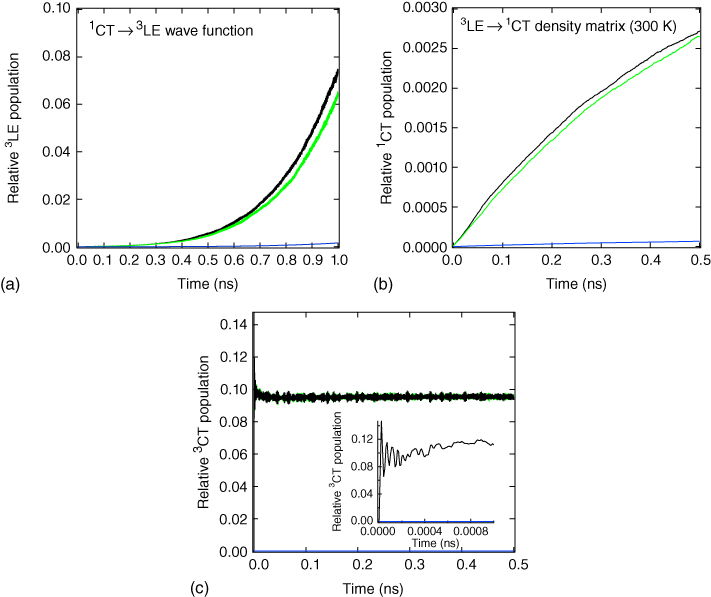
Figure 9.11 (a) Relative populations of the  LE state associated with intersystem crossing after excitation into the
  CT state. (b) The relative populations of the
  CT state associated with reverse intersystem crossing (rISC) after initially populating the
  LE state (300 K). (c) Population kinetics of the
  CT state during the rISC dynamics after initial population of the
  LE state, i.e. (b) inset is a zoom into the early time kinetics. Black: full model Hamiltonian, green: no HFI, and blue: no vibronic coupling.
Figure 9.11b shows the same simulations, but in this case they are initiated in the lowest triplet state, ![]() LE, to mimic the rISC dynamics. These simulations were performed at 300 K, using the density operator formalism of MCTDH described above. As expected, these indicate the same trends as observed in Figure 9.11a. Indeed, if the vibronic coupling between the
LE, to mimic the rISC dynamics. These simulations were performed at 300 K, using the density operator formalism of MCTDH described above. As expected, these indicate the same trends as observed in Figure 9.11a. Indeed, if the vibronic coupling between the ![]() LE and
LE and ![]() CT states is neglected (blue trace), the
CT states is neglected (blue trace), the ![]() is significantly reduced, while exclusion of HFI has almost no effect, despite the near degeneracy of the two CT states.
is significantly reduced, while exclusion of HFI has almost no effect, despite the near degeneracy of the two CT states.
Importantly, the critical role of vibronic coupling between the two triplet states for the ![]() LE
LE ![]() CT conversion cannot be described within a similar first‐order perturbation theory approach. Therefore following the work of Henry and Siebrand [96], a more general expression of the ISC/rISC rate derived from second‐order perturbation theory must be adopted. Here the rISC rate is described as1
CT conversion cannot be described within a similar first‐order perturbation theory approach. Therefore following the work of Henry and Siebrand [96], a more general expression of the ISC/rISC rate derived from second‐order perturbation theory must be adopted. Here the rISC rate is described as1

The first term is the normal first‐order FGR describing the transition from some initial state (![]() ) to a final state (
) to a final state (![]() ). In contrast coupling between the initial and final states in the second term, so‐called second order, is mediated by an intermediate state (
). In contrast coupling between the initial and final states in the second term, so‐called second order, is mediated by an intermediate state (![]() ). In the present case, a direct second‐order coupling would require population transfer between the two CT states, via the HFI, i.e. an initial
). In the present case, a direct second‐order coupling would require population transfer between the two CT states, via the HFI, i.e. an initial ![]() LE state populates the
LE state populates the ![]() CT via vibronic coupling, which decays into the
CT via vibronic coupling, which decays into the ![]() CT, via the HFI. However, as already demonstrated the HFI coupling plays an insignificant role. Consequently, the relevant terms for the present observations are
CT, via the HFI. However, as already demonstrated the HFI coupling plays an insignificant role. Consequently, the relevant terms for the present observations are
and
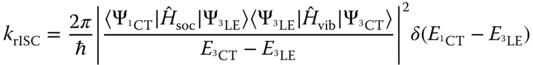
Eqs. (9.34) and (9.35) indicate a two‐step mechanism. Firstly, the large vibronic coupling between ![]() LE and
LE and ![]() CT promotes, on a time scale much faster than the rISC (see Figure 9.11c), an equilibrium between the two states. Obviously, the position of this equilibrium depends both on the size of the vibronic coupling and the energy gap. Subsequently, the second‐order term, Eq. (9.35), couples the
CT promotes, on a time scale much faster than the rISC (see Figure 9.11c), an equilibrium between the two states. Obviously, the position of this equilibrium depends both on the size of the vibronic coupling and the energy gap. Subsequently, the second‐order term, Eq. (9.35), couples the ![]() CT and the
CT and the ![]() CT, using the
CT, using the ![]() LE as an intermediate. This latter second‐order term is very efficient because of the good vibrational overlap between the almost degenerate initial and final states,
LE as an intermediate. This latter second‐order term is very efficient because of the good vibrational overlap between the almost degenerate initial and final states, ![]() CT and
CT and ![]() CT, respectively. Therefore, the two coupling terms driving this dynamics are the SOC and the vibronic coupling elements. This explains recent experimental results that demonstrated that steric hindrance of D–A dihedral angle switches the main pathway from TADF to phosphorescence [21], [39], [97]. This steric hindrance is equivalent to removing the vibronic coupling term, which is shown herein to be the strongest along modes exhibiting a distortion of the D–A dihedral angle.
CT, respectively. Therefore, the two coupling terms driving this dynamics are the SOC and the vibronic coupling elements. This explains recent experimental results that demonstrated that steric hindrance of D–A dihedral angle switches the main pathway from TADF to phosphorescence [21], [39], [97]. This steric hindrance is equivalent to removing the vibronic coupling term, which is shown herein to be the strongest along modes exhibiting a distortion of the D–A dihedral angle.
It is also consistent with the time‐resolved EPR study of Ogiwara et al. [37] who concluded rISC occurring in the spin–orbit and hyperfine pathways. However, the EPR only probes the population of the ![]() LE and
LE and ![]() CT states. For molecules where they found fast rISC, there was significant population of the
CT states. For molecules where they found fast rISC, there was significant population of the ![]() CT. In Ref. [22] they proposed that this population would undergo transfer via HFI interaction, and therefore the two routes for transfer into the
CT. In Ref. [22] they proposed that this population would undergo transfer via HFI interaction, and therefore the two routes for transfer into the ![]() CT state made rISC faster. But as shown in our present work, an equilibrium between the
CT state made rISC faster. But as shown in our present work, an equilibrium between the ![]() LE and
LE and ![]() CT exists and depends on the strength of vibronic coupling. Therefore strong vibronic coupling would increase the population of the
CT exists and depends on the strength of vibronic coupling. Therefore strong vibronic coupling would increase the population of the ![]() CT state and provide rapid rISC, as they observe, via the second‐order mechanism we demonstrated. Therefore again, these results are entirely consistent with our simulations.
CT state and provide rapid rISC, as they observe, via the second‐order mechanism we demonstrated. Therefore again, these results are entirely consistent with our simulations.
In the context of recent results on similar molecules with the D–A–D setup, Santos et al. [97] reported a strong dependence on the relative energy levels according to the environment. This is not surprising given the interplay between CT and LE states, both of which will exhibit different responses to changes in the local embedding environment. This gives rise to three distinct scenarios, shown schematically in Figure 9.12: (i) the LE below the CT states, (ii) the LE degenerate with the CT states, and (iii) the LE above the CT states. Only the first case, the one studied here, requires the initial rIC step, but importantly, because the vibronic coupling is an order of magnitude larger than the other coupling mechanisms, this first step required in Figure 9.12a will be significantly faster than the k![]() process. Indeed, as shown in Figure 9.11c, an equilibrium between the two triplet states is reached very quickly. It therefore is not the rate‐determining step and consequently will not change the overall rate of rISC.
process. Indeed, as shown in Figure 9.11c, an equilibrium between the two triplet states is reached very quickly. It therefore is not the rate‐determining step and consequently will not change the overall rate of rISC.

Figure 9.12 Schematic energy‐level diagrams illustrating the effect to the environment of the relative splitting of the CT and LE states of PTZ‐DBTO2.
Source: Ref. [42]. Reproduced with permission of John Wiley & Sons.
Importantly, this mechanism was recently demonstrated using a combination of photoinduced absorption and quantum dynamics, using the methods described above [98]. By placing the TADF molecule in a solid polar polyethylene oxide (PEO) host, it was shown that the rigidity and polarity of the host greatly affects the rISC rate and thus TADF. By exploiting the temperature‐dependent polarity of the PEO host (Figure 9.13a), the CT states were brought into energetic resonance with the ![]() LE state, and a significant increase in TADF was observed. These results allowed three distinct regimes of TADF to be categorized as TADF I (CT
LE state, and a significant increase in TADF was observed. These results allowed three distinct regimes of TADF to be categorized as TADF I (CT ![]() LE), TADF II (CT = LE), and TADF III (CT
LE), TADF II (CT = LE), and TADF III (CT ![]() LE). These observations were simulated using quantum dynamics (Figure 9.13b) and the model Hamiltonian outlined above showing that vibronic coupling between the local and CT triplet states invokes an efficient second‐order coupling from the triplet states to the singlet CT state. The model predicts the same resonant behavior of TADF as a function of temperature, confirming the proposed model for efficient TADF.
LE). These observations were simulated using quantum dynamics (Figure 9.13b) and the model Hamiltonian outlined above showing that vibronic coupling between the local and CT triplet states invokes an efficient second‐order coupling from the triplet states to the singlet CT state. The model predicts the same resonant behavior of TADF as a function of temperature, confirming the proposed model for efficient TADF.

Figure 9.13 (a) The temperature dependence of the intensity (black line) and CT onset energy (purple circles). The change in CT onset energy plateaus below the glass temperature, representative of the PEO film becoming rigid. The black dashed line represents the energy of the  LE at 2.58 eV, with the peak in intensity apparent as the CT energy crosses resonance. (b) Relative rate of reverse intersystem crossing as a function of temperature for the D–A complex PTZ‐DPTO2. The rates were extracted from the population of the 1CT state at 0.5 ns of dynamics simulations initiated from the lowest triplet state..
Source: Ref. [98]. https://www.nature.com/articles/ncomms13680#rightslink.LicensedUnderCCBY4.0
9.4 Conclusions and Outlook
The importance of a deeper first principles understanding of the properties of TADF emitters should not be underestimated, and in this regard theory and computations play an important role. It is therefore rather surprising that, despite the significant experimental interested in this area, the number of computational studies remains rather small. In this chapter, we have described computational approaches for simulating the excited‐state dynamics of molecules, achieved using model PES and wavepacket dynamics simulations, which achieve a rigorous treatment of motion over this excited‐state surface.
The two case studies used illustrate the importances of explicitly considering the role of excited‐state nuclear motion when trying to establish a detailed understanding of ISC and rISC. As demonstrated in the second case study, this is critically important to describe the rate of efficient rISC in organic TADF molecules. These results, which are consistent with all recent experimental observations, demonstrate the dynamical mechanism of rISC. This also highlights the importance of not just tuning the ![]() gap but paying close attention to the gaps between the
gap but paying close attention to the gaps between the ![]() LE and
LE and ![]() CT and
CT and ![]() CT and
CT and ![]() CT states. There are now two energy gaps to consider! As the relative gaps between the CT and LE states are sensitive to the immediate embedding environment, this opens the ability to tune the performance of molecular emitters within the device by altering the rigidity or polarity of the host molecules. This effect has recently been demonstrated [98], and device tuning in this manner is likely to be crucial for achieving high external quantum efficiencies.
CT states. There are now two energy gaps to consider! As the relative gaps between the CT and LE states are sensitive to the immediate embedding environment, this opens the ability to tune the performance of molecular emitters within the device by altering the rigidity or polarity of the host molecules. This effect has recently been demonstrated [98], and device tuning in this manner is likely to be crucial for achieving high external quantum efficiencies.
Finally, it is clear that for high performing devices, high fluorescence efficiencies are important. But more importantly, the radiative decay rate must be much faster than all nonradiative processes. Therefore, in terms of molecular vibrations, it will be important to identify which vibrational modes control radiative decay rates and rISC and the competition between them and with nonradiative processes, along with the role played by all excited states, including upper excited states, involved in TADF, as a function of molecular geometry and controlled degrees of torsional freedom. We must understand which vibrational modes couple ![]() CT and
CT and ![]() LE and each to the ground state, especially those mediating fast nonradiative decay of the
LE and each to the ground state, especially those mediating fast nonradiative decay of the ![]() CT state and those mediating rISC. This leads to the key question: Can we block the former vibrational channels while retaining the latter and hence efficient TADF? This idea of dynamic molecular optimization also has the potential great ramifications in many different fields of molecular photophysics.
CT state and those mediating rISC. This leads to the key question: Can we block the former vibrational channels while retaining the latter and hence efficient TADF? This idea of dynamic molecular optimization also has the potential great ramifications in many different fields of molecular photophysics.
References
- 1 Burroughes, J.H., Bradley, D.D.C., Brown, A.R., Marks, R.N., Mackay, K., Friend, R.H, Burns, P.L., and Holmes, A.H. (1990). Light emitting diodes based on conjugated polymers. Nature 347: 539–541.
- 2 Wilson, J.S., Dhoot, A.S., Seeley, A.J.A.B., Khan, M.S. and KÖhler, A., and Friend, R.H. (2001). Spin‐dependent exciton formation in ‐conjugated compounds. Nature 413: 828–831.
- 3 Baldo, M.A., O'Brien, D.F., You, Y., Shoustikov, A., Sibley, S., Thompson, M.E., and Forrest, S.R. (1998). Highly efficient phosphorescent emission from organic electroluminescent devices. Nature 395: 151–154.
- 4 Yersin, H. (2004). Triplet emitters for OLED applications. Mechanisms of exciton trapping and control of emission properties. In: Transition Metal and Rare Earth Compounds, Topics in Current Chemistry. 1–26. Berlin: Springer‐Verlag.
- 5 Reineke, S., Walzer, K., and Leo, K. (2007). Triplet exciton quenching in organic phosphorescent light emitting diodes with Ir‐based emitters. Phys. Rev. B 75: 125328.
- 6 Volz, D., Wallesch, M., Flechon, C., Danz, M., Verma, A., Navarro, J.M., Zink, D., Braese, S., and Baumann, T. (2015). From iridium and platinum to copper and carbon: new avenues for more sustainability in organic light‐emitting diodes. Green Chem. 17: 1988–2011.
- 7 Monkowius, U. and Yersin, H. (2010). Komplexe mit kleinen Singulett‐Triplett‐Energie‐Abständen zur Verwendung in opto‐elektronischen Bauteilen (Singulett‐Harvesting‐Effekt) Complexes with small singlet‐triplet energy separations for use in opto‐electronic components (singlet harvesting effect). DE Patent Application DE200,810,033,563.
- 8 Endo, A., Ogasawara, A., Takahashi, A., Yokoyama, D., Kato, Y., and Adachi, C. (2009). Thermally activated delayed fluorescence from Sn–porphyrin complexes and their application to organic light emitting diodes — a novel mechanism for electroluminescence. Adv. Mater. 21: 4802–4806.
- 9 Lee, J., Shizu, K., Tanaka, H., Nomura, H., Yasuda, T., and Adachi, C. (2013). Oxadiazole‐ and triazole‐based highly efficient thermally activated delayed fluorescence emitters for organic light emitting diodes. J. Mater. Chem. C 1: 4599–4604.
- 10 Yersin, H. (2008). Highly Efficient OLEDs with Phosphorescent Materials. Wiley.
- 11 Uoyama, H., Goushi, K., Shizu, K., Nomura, H., and Adachi, C. (2012). Highly efficient organic light‐emitting diodes from delayed fluorescence. Nature 492: 234–238.
- 12 Goushi, K., Yoshida, K., Sato, K., and Adachi, C. (2012). Organic light‐emitting diodes employing efficient reverse intersystem crossing for triplet‐to‐singlet state conversion. Nat. Photonics 6: 253–258.
- 13 Worth, G.A. and Cederbaum, L.S. (2004). Beyond Born–Oppenheimer: molecular dynamics through a conical intersection. Annu. Rev. Phys. Chem. 55: 127–158.
- 14 Berberan‐Santos, M.N. and Garcia, J.M.M. (1996). Unusually strong delayed fluorescence of C70. J. Am. Chem. Soc. 118: 9391–9394.
- 15 Baleizão, C. and Berberan‐Santos, M.N. (2007). Thermally activated delayed fluorescence as a cycling process between excited singlet and triplet states: application to the fullerenes. J. Chem. Phys. 126: 204510.
- 16 Delorme, R. and Perrin, F. (1929). Duration of the fluorescence of solid uranyl salts and their solution. J. Phys. Rad. Ser. 10: 177–186.
- 17 Lewis, G.N., Lipkin, D., and Magel, T.T. (1941). Reversible photochemical processes in rigid media: a study of the phosphorescent state. J. Am. Chem. Soc. 63: 3005–3018.
- 18 Parker, C.A. and Hatchard, C.G. (1961). Triplet‐singlet emission in fluid solutions: phosphorescence of Eosin. Trans. Faraday Soc. 57: 1894–1904.
- 19 Kirchhoff, J.R., Gamache, J.E., Blaskie, M.W., Del‐Paggio, A.A., Lengel, R.K., and McMillin, D.R. (1983). Temperature dependence of luminescence from Cu(NN) systems in fluid solution. Evidence for the participation of two excited states. Inorg. Chem. 22: 2380–2384.
- 20 Zhang, Q., Li, J., Shizu, K., Huang, S., Hirata, S., Miyazaki, H., and Adachi, C. (2012). Design of efficient thermally activated delayed fluorescence materials for pure blue organic light emitting diodes. J. Am. Chem. Soc. 134: 14706–14709.
- 21 Dias, F.B., Bourdakos, K.N., Jankus, V., Moss K.C., Kamtekar, K.T., Bhalla, V., Santos, J., Bryce, M.R., and Monkman, A.P. (2013). Triplet harvesting with 100% efficiency by way of thermally activated delayed fluorescence in charge transfer OLED emitters. Adv. Mater. 25: 3707–3714.
- 22 Dias, F.B. (2015). Kinetics of thermal assisted delayed fluorescence in blue organic emitters with large singlet–triplet energy gap. Philos. Trans. R. Soc. London, Ser. A 373: 20140447.
- 23 Inoue, M., Serevičius, T., Nakanotani, H., Yoshida, K., Matsushima, T., JurS&c.breve;ėnas, S., and Adachi, C. (2016). Effect of reverse intersystem crossing rate to suppress efficiency roll‐off in organic light‐emitting diodes with thermally activated delayed fluorescence emitters. Chem. Phys. Lett. 644: 62–67.
- 24 Marian, C.M. (2011). Spin–orbit coupling and intersystem crossing in molecules. WIREs Comput. Mol. Sci. 2: 187–203.
- 25 Capano, G., Rothlisberger, U., Tavernelli, I., and Penfold, T.J. (2015). Theoretical rationalization of the emission properties of prototypical Cu(I)–phenanthroline complexes. J. Phys. Chem. A 119: 7026–7037.
- 26 Leitl, M.J., Zink, D.M., Schinabeck, A.J., Baumann, T., Volz, D., and Yersin, H. (2016). Copper(I) complexes for thermally activated delayed fluorescence: from photophysical to device properties. Top. Curr. Chem. 374: 1–34.
- 27 Tatchen, J., Gilka, N., and Marian, C.M. (2007). Intersystem crossing driven by vibronic spin–orbit coupling: a case study on psoralen. Phys. Chem. Chem. Phys. 9: 5209–5221.
- 28 Etinski, M., Rai‐Constapel, V., and Marian, C.M. (2014). Time‐dependent approach to spin–vibronic coupling: implementation and assessment. J. Chem. Phys. 140: 114104.
- 29 Marian, C.M., Etinski, M., and Rai‐Constapel, V. (2014). Reverse intersystem crossing in rhodamines by near‐infrared laser excitation. J. Phys. Chem. A 118: 6985–6990.
- 30 Minns, R.S., Parker, D.S.N., Penfold, T.J., Worth, G.A., and Fielding, H.H. (2010). Competing ultrafast intersystem crossing and internal conversion in the “channel 3” region of benzene. Phys. Chem. Chem. Phys. 12: 15607–15615.
- 31 Penfold, T.J., Spesyvtsev, R., Kirkby, O.M., Minns, R.S., Parker, D.N.S., Fielding, H.H., and Worth, G.A. (2012). Quantum dynamics study of the competing ultrafast intersystem crossing and internal conversion in the “channel 3” region of benzene. J. Chem. Phys. 137: 204310.
- 32 Capano, G., Chergui, M., Rothlisberger, U., Tavernelli, I., and Penfold, T.J. (2014). A quantum dynamics study of the ultrafast relaxation in a prototypical Cu(I)–phenanthroline. J. Phys. Chem. A 118: 9861–9869.
- 33 Lim, B.T., Okajima, S., Chandra, A.K., and Lim, A.C. (1981). Radiationless transitions in electron donor‐acceptor complexes: selection rules for S‐T intersystem crossing and efficiency of S‐S internal conversion. Chem. Phys. Lett. 79: 22–27.
- 34 El‐Sayed, M.A. (1963). Spin–orbit coupling and the radiationless processes in nitrogen heterocyclics. J. Chem. Phys. 38: 2834–2838.
- 35 Dias, F.B., Santos, J., Graves, D., Data, P., Nobuyasu, R.S., Fox, M.S., Batsanov, A.S., Palmeira, T., Berberan‐Santos, M.N., Bryce, M.R., and Monkman, A.P. (2016). The role of local triplet excited states and D‐A relative orientation in thermally activated delayed fluorescence: photophysics and devices. Adv. Sci. doi: 10.13140/RG.2.1.1821.1446.
- 36 Chen, X.K., Zhang, S.F., Fan, J.X., and Ren, A.M. (2015). Nature of highly efficient thermally activated delayed fluorescence in OLED emitters: non adiabatic effect between excited states. J. Phys. Chem. C 119: 9728–9733.
- 37 Ogiwara, T., Wakikawa, Y., and Ikoma, T. (2015). Mechanism of intersystem crossing of thermally activated delayed fluorescence molecules. J. Phys. Chem. A 119: 3415–3418.
- 38 Hontz, E., Chang, W., Congreve, D.N., Bulovic, V., Baldo, M.A., and Van‐Voorhis, T. (2015). The role of electron–hole separation in thermally activated delayed fluorescence in donor–acceptor blends. J. Phys. Chem. C 119: 25591–25597.
- 39 Ward, J.S., Nobuyasu, R.S., Batsanov, A.S., Data, P., Monkman, A.P., Dias, F.B., and Bryce, M.R. (2016). The interplay of thermally activated delayed fluorescence (TADF) and room temperature organic phosphorescence in sterically‐constrained donor–acceptor charge‐transfer molecules. Chem. Commun. 52: 2612–2615.
- 40 Marian, C.M. (2016). On the mechanism of the triplet‐to‐singlet upconversion in the assistant dopant ACRXTN. J. Phys. Chem. C 120: 3715–3721.
- 41 Sousa, C., de Graaf, C., Rudavskyi, A., Broer, R., Tatchen, J., Etinski, M., and Marian, C.M. (2013). Ultrafast deactivation mechanism of the excited singlet in the light‐induced spin crossover of [Fe(2,2‐bipyridine)]. Chem. Eur. J. 19: 17541–17551.
- 42 Gibson, J., Monkman, A.P., and Penfold, T.J. (2016). The importance of vibronic coupling for efficient reverse intersystem crossing in TADF molecules. ChemPhysChem doi: 10.1002/cphc.201600662.
- 43 Born, M. and Huang, K. (1998). Dynamical Theory of Crystal Lattices. Oxford University Press.
- 44 Raab, A., Worth, G.A., Meyer, H.‐D., and Cederbaum, L.S. (1999). Molecular dynamics of pyrazine after excitation to the S electronic state using a realistic 24‐mode model Hamiltonian. J. Chem. Phys. 110: 936–946.
- 45 Markmann, A., Worth, G.A., and Cederbaum, L.S. (2005). Allene and pentatetraene cations as models for intramolecular charge transfer: vibronic coupling Hamiltonian and conical intersections. J. Chem. Phys. 122: 144320.
- 46 Worth, G.A., Welch, G., and Paterson, M.J. (2006). Wavepacket dynamics study of Cr(CO) after formation by photodissociation: relaxation through an (ExA)xe Jahn‐Teller conical intersection. Mol. Phys. 104: 1095–1105.
- 47 Pápai, M., Rozgonyi, T., Vanko, G., and Penfold, T.J. (2016). High efficiency iron photosensitiser explained with quantum wavepacket dynamics. J. Phys. Chem. Lett. 7: 2009–2014.
- 48 Car, R. and Parrinello, M. (1985). Unified approach for molecular dynamics and density‐functional theory. Phys. Rev. Lett. 55: 2471–2474.
- 49 Curchod, B.F.E., Rothlisberger, U., and Tavernelli, I. (2013). Trajectory‐based nonadiabatic dynamics with time‐dependent density functional theory. ChemPhysChem 14: 1314–1340.
- 50 Richings, G.W., Polyak, I., Spinlove, K.E., Worth, G.A., Burghardt, I., and Lasorne, B. (2015). Quantum dynamics simulations using gaussian wavepackets: the vMCG method. Int. Rev. Phys. Chem. 34: 269–308.
- 51 Wang, L., Akimov, A.V., and Prezhdo, O.V. (2016). Recent progress in surface hopping: 2011–2015. J. Phys. Chem. Lett. 7: 2100–2112.
- 52 Tully, J.C. and Preston, R.K. (1971). Trajectory surface hopping approach to nonadiabatic molecular collisions: the reaction of H with D. J. Chem. Phys. 55: 562–572.
- 53 Tully, J.C. (1990). Molecular dynamics with electronic transitions. J. Chem. Phys. 93: 1061–1071.
- 54 Köppel, H., Domcke, W., and Cederbaum, L.S. (1984). Multimode molecular dynamics beyond the Born‐Oppenheimer approximation. Adv. Chem. Phys. 57: 59–246.
- 55 Cattarius, C., Worth, G.A., Meyer, H.‐D., and Cederbaum, L.S. (2001). All mode dynamics at the conical intersection of an octa‐atomic molecule: multi‐configuration time‐dependent Hartree (MCTDH) investigation on the butatriene cation. J. Chem. Phys. 115: 2088–2100.
- 56 Mahapatra, S., Cederbaum, L.S., and Koppel, H. (1999). Theoretical investigation of Jahn‐Teller and Pseudo‐Jahn‐Teller coupling effects on the photoelectron spectrum of allene. J. Chem. Phys. 111: 10452–10463.
- 57 Penfold, T.J. and Worth, G.A. (2009). A model Hamiltonian to simulate the complex photochemistry of benzene II. J. Chem. Phys. 131: 190–199.
- 58 Barbatti, M. (2011). Nonadiabatic dynamics with trajectory surface hopping method. WIREs Comput. Mol. Sci. 1: 620–633.
- 59 Martinez, T.J., Ben‐Nun, M., and Levine, R.D. (1996). Multi‐electronic‐state molecular dynamics: a wave function approach with applications. J. Phys. Chem. 100: 7884–7895.
- 60 Ben‐Nun, M. and Martınez, T.J. (1998). Nonadiabatic molecular dynamics: validation of the multiple spawning method for a multidimensional problem. J. Phys. Chem. 108: 7244–7257.
- 61 Shalashilin, D.V. and Child, M.S. (2004). The phase space CCS approach to quantum and semiclassical molecular dynamics for high‐dimensional systems. Chem. Phys. 304: 103–120.
- 62 Shalashilin, D.V. (2009). Quantum mechanics with the basis set guided by Ehrenfest trajectories: theory and application to spin‐boson model. J. Chem. Phys. 130: 244101.
- 63 Worth, G.A. and Burghardt, I. (2003). Full quantum mechanical molecular dynamics using Gaussian wavepackets. Chem. Phys. Lett. 368: 502–508.
- 64 Makhov, D.V., Glover, W.J., Martinez, T.J., and Shalashilin, D.V. (2014). Ab initio multiple cloning algorithm for quantum nonadiabatic molecular dynamics. J. Chem. Phys. 141: 054110.
- 65 McLachlan, A.D. (1964). A variational solution of the time‐dependent Schrodinger equation. Mol. Phys. 8: 39–44.
- 66 Makri, N. and Miller, W.H. (1987). Time‐dependent self‐consistent field (TDSCF) approximation for a reaction coordinate coupled to a harmonic bath: single and multiple configuration treatments. J. Chem. Phys. 87: 5781–5787.
- 67 Beck, M.H., Jäckle, A., Worth, G.A., and Meyer, H.‐D. (2000). The multiconfiguration time‐dependent Hartree method: a highly efficient algorithm for propagating wavepackets. Phys. Rep. 324: 1–105.
- 68 Meyer, H.‐D., Gatti, F., and Worth, G.A. (2008). High Dimensional Quantum Dynamics: Basic Theory, Extensions, and Applications of the MCTDH Method. Weinheim: VCH.
- 69 Tannor, D.J. (2007). Introduction to Quantum Mechanics: A Time Dependent Perspective. University Science Books.
- 70 Raab, A., Burghardt, I., and Meyer, H.‐D. (1999). The multiconfiguration time‐dependent Hartree method generalized to the propagation of density operators. J. Chem. Phys. 111: 8759–8772.
- 71 Raab, A. and Meyer, H.‐D. (2000). Multiconfigurational expansions of density operators: equations of motion and their properties. Theor. Chem. Acc. 104: 358–369.
- 72 Penfold, T.J., Karlsson, S., Capano, G., Lima, F.A., Rittmann, J., Reinhard, M., Rittmann‐Frank, M.H., Braem, O., Baranoff, E., Abela, R., Tavernelli, I., Rothlisberger, U., Milne, C.J., and Chergui, M. (2013). Solvent‐induced luminescence quenching: static and time‐resolved X‐ray absorption spectroscopy of a copper(I) phenanthroline complex. J. Phys. Chem. A 117: 4591–4601.
- 73 Capano, G., Penfold, T.J., Rothlisberger, U., and Tavernelli, I. (2014). A vibronic coupling Hamiltonian to describe the ultrafast excited state dynamics of a Cu(I)–phenanthroline complex. Chimia 68: 227–230.
- 74 Deaton, J.C., Switalski, S.C., Kondakov, D.Y., Young, R.H., Pawlik, T.D., Giesen, D.J., Harkins, S.B., Miller, A.J.M., Mickenberg, S.F., and Peters, J.C. (2010). E‐type delayed fluorescence of a phosphine‐supported Cu(‐NAr) diamond core: harvesting singlet and triplet excitons in OLEDs. J. Am. Chem. Soc. 132: 9499–9508.
- 75 Wallesch, M., Volz, D., Zink, D.M., Schepers, U., Nieger, M., Baumann, T., and Bräse, S. (2014). Bright coppertunities: multinuclear Cu(I) complexes with N‐P ligands and their applications. Chem. Eur. J. 20: 6578–6590.
- 76 Dumur, F. (2015). Recent advances in organic light emitting devices comprising copper complexes: a realistic approach for low cost and highly emissive devices? Org. Electron. 21: 27–39.
- 77 McMillin, D.R., Kirchhoff, J.R., and Goodwin, K.V. (1985). Exciplex quenching of photo‐excited copper complexes. Coord. Chem. Rev. 64: 83–92.
- 78 Armaroli, N. (2001). Photoactive mono‐ and polynuclear Cu(I)–phenanthrolines. A viable alternative to Ru(II)‐polypyridines? Chem. Soc. Rev. 30: 113–124.
- 79 Zgierski, M.Z. (2003). Cu(I)‐2,9‐dimethyl‐1,10‐phenanthroline: density functional study of the structure, vibrational force‐field, and excited electronic states. J. Chem. Phys. 118: 4045.
- 80 Siddique, Z.A., Yamamoto, Y., Ohno, T., and Nozaki, K. (2003). Structure‐dependent photophysical properties of singlet and triplet metal‐to‐ligand charge transfer states in copper(I) bis(diimine) compounds. Inorg. Chem. 42: 6366–6378.
- 81 Chen, L.X., Shaw, G.B., Novozhilova, I., Liu, T., Jennings, G., Attenkofer, K., Meyer, G.J., and Coppens, P. (2003). MLCT state structure and dynamics of a copper(I) diimine complex characterized by pump‐probe X‐ray and laser spectroscopies and DFT calculations. J. Am. Chem. Soc. 125: 7022–7034.
- 82 Iwamura, M., Takeuchi, S., and Tahara, T. (2007). Real‐time observation of the photoinduced structural change of bis(2,9‐dimethyl‐1,10‐phenanthroline)copper(I) by femtosecond fluorescence fpectroscopy: a realistic potential curve of the Jahn‐Teller distortion. J. Am. Chem. Soc. 129: 5248–5256.
- 83 Iwamura, M., Watanabe, H., Ishii, K., Takeuchi, S., and Tahara, T. (2011). Coherent nuclear dynamics in ultrafast photoinduced structural change of bis(diimine) copper(I) complex. J. Am. Chem. Soc. 133: 7728–7736.
- 84 Huang, J., Buyukcakir, O., Mara, M.W., Takeuchi, S., and Tahara, T. (2012). Highly efficient ultrafast electron injection from the singlet MLCT excited state of copper(I) diimine complexes to TiO nanoparticles. Angew. Chem. Int. Ed. 51: 12711–12715.
- 85 Iwamura, M., Takeuchi, S., and Tahara, T. (2014). Substituent effect on the photoinduced structural change of Cu(I) complexes observed by femtosecond emission spectroscopy. Phys. Chem. Chem. Phys. 16: 4143–4154.
- 86 Shaw, G.B., Grant, C.D., Shirota, H., Castner, E.W., Meyer, G.J., and Chen, L.X. (2007). Ultrafast structural rearrangements in the MLCT excited state for copper(I) bis‐phenanthrolines in solution. J. Am. Chem. Soc. 129: 2147–2160.
- 87 Huang, J., Buyukcakir, O., Mara, M.W., Coskun, A., Dimitrijevic, N.M., Barin, G., Kokhan, O., Stickrath, A.B., Ruppert, R., Tiede, D.M., Chen, L.X. (2012). Highly efficient ultrafast electron injection from the singlet MLCT excited state of copper(I) diimine complexes to TiO nanoparticles. Angew. Chem. Int. Ed. 51: 12711–12715.
- 88 Masui, K., Nakanotani, H., and Adachi, C. (2013). Analysis of exciton annihilation in high‐efficiency sky‐blue organic light‐emitting diodes with thermally activated delayed fluorescence. Org. Electron. 14: 2721–2726.
- 89 Nobuyasu, R.S., Ren, Z., Griffiths, G.C., Batsanov, A.S., Data, P., Yan, S., Monkman, A.P., Bryce, M.R., and Dias, F.B. (2016). Rational design of TADF polymers using donor–acceptor monomer with enhanced TADF efficiency induced by the energy alignment of charge transfer and local triplet excited states. Adv. Opt. Mater. 4: 597–607.
- 90 Zhao, Y. and Truhlar, D.G. (2008). The M06 suite of density functionals for main group thermochemistry, thermochemical kinetics, noncovalent interactions, excited states, and transition elements: two new functionals and systematic testing of four M06‐class functionals and 12 other functionals. Theor. Chem. Acc. 120: 215–241.
- 91 Hirata, S. and Head‐Gordon, M. (1999). Time‐dependent density functional theory within the Tamm–Dancoff approximation. Chem. Phys. Lett. 314: 291–299.
- 92 Dreuw, A., Weisman, J.L., and Head‐Gordon, M. (2003). Long‐range charge‐transfer excited states in time‐dependent density functional theory require non‐local exchange. J. Chem. Phys. 119: 2943–2946.
- 93 Li, R., Zheng, J., and Truhlar, D.G. (2010). Density functional approximations for charge transfer excitations with intermediate spatial overlap. Phys. Chem. Chem. Phys. 12: 12697–12701.
- 94 Penfold, T.J. (2015). On predicting the excited‐state properties of thermally activated delayed fluorescence emitters. J. Phys. Chem. C 119: 13535–13544.
- 95 Peach, M.J.G., Williamson, M.J., and Tozer, D.J. (2011). Influence of triplet instabilities in TDDFT. J. Comput. Theor. Chem. 7: 3578–3585.
- 96 Henry, B.R. and Siebrand, W. (1971). Spin–Orbit coupling in aromatic hydrocarbons: analysis of nonradiative transitions between singlet and triplet states in benzene and naphthalene. J. Chem. Phys. 54: 1072–1085.
- 97 Santos, P.L., Ward, J.S., Data, P., Batsanov, A.S., Bryce, M.R., Dias, F.B., and Monkman, A.P. (2016). Engineering the singlet–triplet energy splitting in a TADF molecule. J. Mater. Chem. C 4: 3815–3824.
- 98 Etherington, M.K., Gibson, J., Higginbotham, H.F., Penfold, T.J., and Monkman, A.P. (2016). Revealing the spin–vibronic coupling mechanism of thermally‐activated delayed fluorescence. Nat. Commun. 7: 13680.