

IBM DB2 for i
This chapter describes what is new for DB2 for i and discusses the following topics:
5.1 Introduction: Getting around with data
DB2 for i is a member of the IBM leading-edge family of DB2 products. It has always been known and appreciated for its ease of use and simplicity. It supports a broad range of applications and development environments.
Because of its unique and self-managing computing features, the cost of ownership of DB2 for i is a valuable asset. The sophisticated cost-based query optimizer, the unique single level store architecture of the OS, and the database parallelism feature of DB2 for i allow it to scale almost linearly. Rich SQL support makes not only it easier for software vendors to port their applications and tools to IBM i, but it also enables developers to use industry-standard SQL for their data access and programming. The IBM DB2 Family has this focus on SQL standards with DB2 for i, so investment in SQL enables DB2 for i to use the relational database technology leadership position of IBM and maintain close compatibility with the other DB2 Family products.
Reading through this chapter, you find many modifications and improvements as part of the new release. All of these features are available to any of the development and deployment environments that are supported by the IBM Power platforms on which IBM i 7.1 can be installed.
Many DB2 enhancements for IBM i 7.1 are also available for Version 6.1. If you must verify their availability, go to:
This link takes you to the DB2 for i section of the IBM i Technology Updates wiki.
5.2 SQL data description and data manipulation language
There are several changes and additions to the SQL language:
5.2.1 XML support
Extensible Markup Language (XML) is a simple and flexible text format that is derived from SGML (ISO 8879). Originally designed to meet the challenges of large-scale electronic publishing, XML is also playing an increasingly important role in the exchange of a wide variety of data on the web and elsewhere.
For more information about XML, go to:
Previously, XML data types were supported only through user-defined types and any handling of XML data was done using user-defined functions. In IBM i 7.1, the DB2 component is complemented with support for XML data types and publishing functions. It also supports XML document and annotation, document search (IBM OmniFind®) without decomposition, and client and language API support for XML (CLI, ODBC, JDBC, and so on).
For more information about moving from the user-defined function support provided through the XML Extenders product to the built-in operating support, see the Replacing DB2 XML Extender With integrated IBM DB2 for i XML capabilities white paper:
XML data type
An XML value represents well-formed XML in the form of an XML document, XML content, or an XML sequence. An XML value that is stored in a table as a value of a column that is defined with the XML data type must be a well-formed XML document. XML values are processed in an internal representation that is not comparable to any string value, including another XML value. The only predicate that can be applied to the XML data type is the IS NULL predicate.
An XML value can be transformed into a serialized string value that represents an XML document using the XMLSERIALIZE (see “XML serialization” on page 163) function. Similarly, a string value that represents an XML document can be transformed into an XML value using the XMLPARSE (see “XML publishing functions” on page 162) function. An XML value can be implicitly parsed or serialized when exchanged with application string and binary data types.
The XML data type has no defined maximum length. It does have an effective maximum length of 2 GB when treated as a serialized string value that represents XML, which is the same as the limit for Large Object (LOB) data types. Like LOBs, there are also XML locators and XML file reference variables.
With a few exceptions, you can use XML values in the same contexts in which you can use other data types. XML values are valid in the following circumstances:
•CAST a parameter marker, XML, or NULL to XML
•XMLCAST a parameter marker, XML, or NULL to XML
•IS NULL predicate
•COUNT and COUNT_BIG aggregate functions
•COALESCE, IFNULL, HEX, LENGTH, CONTAINS, and SCORE scalar functions
•XML scalar functions
•A SELECT list without DISTINCT
•INSERT VALUES clause, UPDATE SET clause, and MERGE
•SET and VALUES INTO
•Procedure parameters
•User-defined function arguments and result
•Trigger correlation variables
•Parameter marker values for a dynamically prepared statement
XML values cannot be used directly in the following places. Where expressions are allowed, an XML value can be used, for example, as the argument of XMLSERIALIZE.
•A SELECT list that contains the DISTINCT keyword
•A GROUP BY clause
•An ORDER BY clause
•A subselect of a fullselect that is not UNION ALL
•A basic, quantified, BETWEEN, DISTINCT, IN, or LIKE predicate
•An aggregate function with the DISTINCT keyword
•A primary, unique, or foreign key
•A check constraint
•An index column
No host languages have a built-in data type for the XML data type.
XML data can be defined with any EBCDIC single byte or mixed CCSID or a Unicode CCSID of 1208 (UTF-8), 1200 (UTF-16), or 13488 (Unicode-specific version). 65535 (no conversion) is not allowed as a CCSID value for XML data. The CCSID can be explicitly specified when you define an XML data type. If it is not explicitly specified, the CCSID is assigned using the value of the SQL_XML_DATA_CCSID QAQQINI file parameter (5.3.17, “QAQQINI properties” on page 200). If this value is not set, the default is 1208. The CCSID is established for XML data types that are used in SQL schema statements when the statement is run.
XML host variables that do not have a DECLARE VARIABLE that assigns a CCSID have their CCSID assigned as follows:
•If it is XML AS DBCLOB, the CCSID is 1200.
•If it is XML AS CLOB and the SQL_XML_DATA_CCSID QAQQINI value is 1200 or 13488, the CCSID is 1208.
•Otherwise, the SQL_XML_DATA_CCSID QAQQINI value is used as the CCSID.
Because all implicit and explicit XMLPARSE functions are run by using UTF-8 (1208), defining data in this CCSID removes the need to convert the data to UTF-8.
XML publishing functions
Table 5-1 describes the functions that are directly used in a SQL query.
Table 5-1 XML publishing functions
|
Function
|
Description
|
|
xmlagg
|
Combines a collection of rows, each containing a single XML value to create an XML sequence that contains an item for each non-null value in a set of XML values.
|
|
xmlattributes
|
Returns XML attributes from columns, using the name of each column as the name of the corresponding attribute.
|
|
xmlcomment
|
Returns an XML value with the input argument as the content.
|
|
xmlconcat
|
Returns a sequence that contains the concatenation of a variable number of XML input arguments.
|
|
xmldocument
|
Returns an XML document.
|
|
xmlelement
|
Returns an XML element.
|
|
xmforest
|
Returns an XML value that is a sequence of XML element nodes.
|
|
xmlgroup
|
Returns a single top-level element to represent a table or the result of a query.
|
|
xmlnamespaces
|
Constructs namespace declarations from the arguments.
|
|
xmlparse
|
Parses the arguments as an XML document and returns an XML value.
|
|
xmlpi
|
Returns an XML value with a single processing instruction.
|
|
xmlrow
|
Returns a sequence of row elements to represent a table or the result of a query.
|
|
xmlserialize
|
Returns a serialized XML value of the specified data type generated from the XML-expression argument.
|
|
xmltext
|
Returns an XML value that has the input argument as the content.
|
|
xmlvalidate
|
Returns a copy of the input XML value that is augmented with information obtained from XML schema validation, including default values and type annotations.
|
|
xsltransform
|
Converts XML data into other forms, accessible for the XSLT processor, including but not limited to XML, HTML, and plain text.
|
You can use the SET CURRENT IMPLICIT XMLPARSE OPTION statement to change the value of the CURRENT IMPLICIT XMLPARSE OPTION special register to STRIP WHITESPACE or to PRESERVE WHITESPACE for your connection. You can either remove or maintain any white space on an implicit XMLPARSE function. This statement is not a committable operation.
XML serialization
XML serialization is the process of converting XML data from the format that it has in a DB2 database to the serialized string format that it has in an application.
You can allow the DB2 database manager to run serialization implicitly, or you can start the XMLSERIALIZE function to request XML serialization explicitly. The most common usage of XML serialization is when XML data is sent from the database server to the client.
Implicit serialization is the preferred method in most cases because it is simpler to code, and sending XML data to the client allows the DB2 client to handle the XML data properly. Explicit serialization requires extra handling, which is automatically handled by the client during implicit serialization.
In general, implicit serialization is preferable because it is more efficient to send data to the client as XML data. However, under certain circumstances (for example, if the client does not support XML data) it might be better to do an explicit XMLSERIALIZE.
With implicit serialization for DB2 CLI and embedded SQL applications, the DB2 database server adds an XML declaration with the appropriate encoding specified to the data. For .NET applications, the DB2 database server also adds an XML declaration. For Java applications, depending on the SQLXML object methods that are called to retrieve the data from the SQLXML object, the data with an XML declaration added by the DB2 database server is returned.
After an explicit XMLSERIALIZE invocation, the data has a non-XML data type in the database server, and is sent to the client as that data type. You can use the XMLSERIALIZE scalar function to specify the SQL data type to which the data is converted when it is serialized (character, graphic, or binary data type) and whether the output data includes the explicit encoding specification (EXCLUDING XMLDECLARATION or INCLUDING XMLDECLARATION). The best data type to which to convert XML data is the BLOB data type because retrieval of binary data results in fewer encoding issues. If you retrieve the serialized data into a non-binary data type, the data is converted to the application encoding, but the encoding specification is not modified. Therefore, the encoding of the data most likely does not agree with the encoding specification. This situation results in XML data that cannot be parsed by application processes that rely on the encoding name.
Although implicit serialization is preferable because it is more efficient, you can send data to the client as XML data. When the client does not support XML data, you can consider doing an explicit XMLSERIALIZE. If you use implicit XML serialization for this type of client, the DB2 database server then converts the data to a CLOB (Example 5-1) or DBCLOB before it sends the data to the client.
Example 5-1 XMLSERIALIZE
SELECT e.empno, e.firstnme, e.lastname,
XMLSERIALIZE(XMLELEMENT(NAME "xmp:Emp",
XMLNAMESPACES('http://www.xmp.com' as "xmp"),
XMLATTRIBUTES(e.empno as "serial"),
e.firstnme, e.lastname
OPTION NULL ON NULL))
AS CLOB(1000) CCSID 1208
INCLUDING XMLDECLARATION) AS "Result"
FROM employees e WHERE e.empno = 'A0001'
Managing XML schema repositories (XSR)
The XML schema repository (XSR) is a set of tables that contain information about XML schemas. XML instance documents might contain a reference to a Uniform Resource Identifier (URI) that points to an associated XML schema. This URI is required to process the instance documents. The DB2 database system manages dependencies on externally referenced XML artifacts with the XSR without requiring changes to the URI location reference.
Without this mechanism to store associated XML schemas, an external resource might not be accessible when needed by the database. The XSR also removes the additional impact that is required to locate external documents, along with the possible performance impact.
An XML schema consists of a set of XML schema documents. To add an XML schema to the DB2 XSR, you register XML schema documents to DB2 by calling the DB2 supplied stored procedure SYSPROC.XSR_REGISTER to begin registration of an XML schema.
The SYSPROC.XSR_ADDSCHEMADOC procedure adds more XML schema documents to an XML schema that you are registering. You can call this procedure only for an existing XML schema that is not yet complete.
Calling the SYSPROC.XSR_COMPLETE procedure completes the registration of an XML schema. During XML schema completion, DB2 resolves references inside XML schema documents to other XML schema documents. An XML schema document is not checked for correctness when you register or add documents. Document checks are run only when you complete the XML schema registration.
To remove an XML schema from the DB2 XML schema repository, you can call the SYSPROC.XSR_REMOVE stored procedure or use the DROP XSROBJECT SQL statement.
|
More considerations: Because an independent auxiliary storage pool (IASP) can be switched between multiple systems, there are more considerations for administering XML schemas on an IASP. Use of an XML schema must be contained on the independent ASP where it was registered. You cannot reference an XML schema that is defined in an independent ASP group or in the system ASP when the job is connected to the independent ASP.
|
Annotated XML schema decomposition
Annotated XML schema decomposition, also referred to as decomposition or shredding, is the process of storing content from an XML document in columns of relational tables. Annotated XML schema decomposition operates based on annotations that are specified in an XML schema. After an XML document is decomposed, the inserted data has the SQL data type of the column into which it is inserted.
An XML schema consists of one or more XML schema documents. In annotated XML schema decomposition, or schema-based decomposition, you control decomposition by annotating a document’s XML schema with decomposition annotations. These annotations specify the following details:
•The name of the target table and column in which the XML data is to be stored
•The default SQL schema for when an SQL schema is not identified
•Any transformation of the content before it is stored
The annotated schema documents must be stored in and registered with the XSR. The schema must then be enabled for decomposition. After the successful registration of the annotated schema, decomposition can be run by calling the decomposition stored procedure SYSPROC.XDBDECOMPXML.
The data from the XML document is always validated during decomposition. If information in an XML document does not comply with its specification in an XML schema, the data is not inserted into the table.
Annotated XML schema decomposition can become complex. To make the task more manageable, take several things into consideration. Annotated XML schema decomposition requires you to map possible multiple XML elements and attributes to multiple columns and tables in the database. This mapping can also involve transforming the XML data before you insert it, or apply conditions for insertion.
Here are items to consider when you annotate your XML schema:
•Understand what decomposition annotations are available to you.
•Ensure, during mapping, that the type of the column is compatible with the XML schema type of the element or attribute to which it is being mapped.
•Ensure complex types that are derived by restriction or extension are properly annotated.
•Confirm that no decomposition limits and restrictions are violated.
•Ensure that the tables and columns that are referenced in the annotation exist at the time the schema is registered with the XSR.
XML decomposition enhancements (order of result rows)
In IBM i 7.1, a series of decomposition annotations are provided to define how to decompose an XML document into relational database tables, such as db2-xdb:defaultSQLSchema or db2-xdb:rowSet, db2-xdb:column.
In one XSR, multiple target tables can be specified, so data in an XML document can be shredded to more than one target tables using one XSR. But the order of insertion into tables cannot be specified with existing decomposition annotations. Therefore, if the target tables have a reference relationship, the insertion of dependent row fails if its parent row is not inserted before it.
Two new annotations are supported:
•db2-xdb:order
The db2-xdb:order annotation specifies the insertion order of rows among different tables.
•db2-xdb:rowSetOperationOrder
The db2-xdb:rowSetOperationOrder annotation is a parent for one or more
db2-xdb:order elements.
db2-xdb:order elements.
Using db2-xdb:order and db2-xdb:rowSetOperationOrder is needed only when referential integrity constraints exist in target tables and you try to decompose to them using one XSR.
5.2.2 The MERGE statement
This statement enables the simplification of matching rows in tables so that you can use a single statement that updates a target (a table or view) using data from a source (result of a table reference). Rows might be inserted, updated, or deleted in the target row, as specified by the matching rules. If you insert, update, or delete rows in a view, without an INSTEAD OF trigger, it updates, deletes, or inserts the row into the tables on which the view is based.
More than one modification-operation (UPDATE, DELETE, or INSERT) or signal-statement can be specified in a single MERGE statement. However, each row in the target can be operated on only once. A row in the target can be identified only as MATCHED with one row in the result table of the table-reference. A nested SQL operation (RI or trigger except INSTEAD OF trigger) cannot specify the target table (or a table within the same hierarchy) as a target of an UPDATE, DELETE, INSERT, or MERGE statement. This statement is also often referred to as an upsert.
Using the MERGE statement is potentially good in a Business Intelligence data load scenario, where it can be used to populate the data in both the fact and the dimension tables upon a refresh of the data warehouse. It can also be used for archiving data.
In Example 5-2, the MERGE statement updates the list of activities that are organized by Group A in the archive table. It deletes all outdated activities and updates the activities information (description and date) in the archive table if they were changed. It inserts new upcoming activities into the archive, signals an error if the date of the activity is not known, and requires that the date of the activities in the archive table be specified.
Example 5-2 UPDATE or INSERT activities
MERGE INTO archive ar
USING (SELECT activity, description, date, last_modified
FROM activities_groupA) ac
ON (ar.activity = ac.activity) AND ar.group = 'A'
WHEN MATCHED AND ac.date IS NULL THEN
SIGNAL SQLSTATE '70001'
SET MESSAGE_TEXT =
ac.activity CONCAT ' cannot be modified. Reason: Date is not known'
WHEN MATCHED AND ac.date < CURRENT DATE THEN
DELETE
WHEN MATCHED AND ar.last_modified < ac.last_modified THEN
UPDATE SET
(description, date, last_modified) = (ac.description, ac.date, DEFAULT)
WHEN NOT MATCHED AND ac.date IS NULL THEN
SIGNAL SQLSTATE '70002'
SET MESSAGE_TEXT =
ac.activity CONCAT ' cannot be inserted. Reason: Date is not known'
WHEN NOT MATCHED AND ac.date >= CURRENT DATE THEN
INSERT
(group, activity, description, date)
VALUES ('A', ac.activity, ac.description, ac.date)
ELSE IGNORE
Each group has an activities table. For example, activities_groupA contains all activities Group A organizes, and the archive table contains all upcoming activities that are organized by groups in the company. The archive table has (group, activity) as the primary key, and date is not nullable. All activities tables have activity as the primary key. The last_modified column in the archive is defined with CURRENT TIMESTAMP as the default value.
There is a difference in how many updates are done depending on whether a NOT ATOMIC MERGE or an ATOMIC MERGE was specified:
•In an ATOMIC MERGE, the source rows are processed as though a set of rows is processed by each WHEN clause. Thus, if five rows are updated, any row level update trigger is fired five times for each WHEN clause. This situation means that n statement level update triggers are fired, where n is the number of WHEN clauses that contain an UPDATE, including any WHEN clause that contains an UPDATE that did not process any of the source rows.
•In a NOT ATOMIC MERGE setting, each source row is processed independently as though a separate MERGE statement ran for each source row, meaning that, in the previous case, the triggers are fired only five times.
After running a MERGE statement, the ROW_COUNT statement information item in the SQL Diagnostics Area (or SQLERRD(3) of the SQLCA) is the number of rows that are operated on by the MERGE statement, excluding rows that are identified by the ELSE IGNORE clause.
The ROW_COUNT item and SQLERRD(3) do not include the number of rows that were operated on as a result of triggers. The value in the DB2_ROW_COUNT_SECONDARY statement information item (or SQLERRD(5) of the SQLCA) includes the number of these rows.
No attempt is made to update a row in the target that did not exist before the MERGE statement ran. No updates of rows were inserted by the MERGE statement.
If COMMIT(*RR), COMMIT(*ALL), COMMIT(*CS), or COMMIT(*CHG) is specified, one or more exclusive locks are acquired during the execution of a successful insert, update, or delete. Until the locks are released by a commit or rollback operation, an inserted or updated row can be accessed only by either the application process that ran the insert or update or by another application process using COMMIT(*NONE) or COMMIT(*CHG) through a read-only operation.
If an error occurs during the operation for a row of source data, the row being processed at the time of the error is not inserted, updated, or deleted. Processing of an individual row is an atomic operation. Any other changes that are previously made during the processing of the MERGE statement are not rolled back. If CONTINUE ON EXCEPTION is specified, execution continues with the next row to be processed.
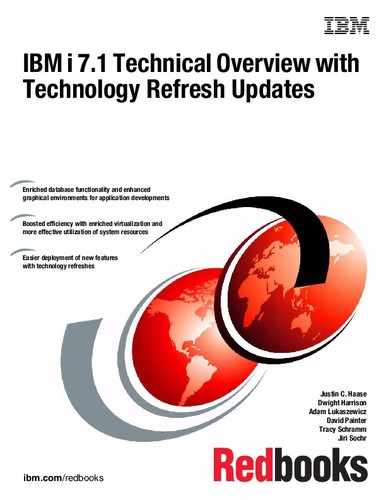
5.2.3 Dynamic compound statements
A dynamic compound statement starts with a BEGIN, has a middle portion similar to an SQL procedure, and ends with an END. It can be executed through any SQL dynamic interface such as the Run SQL Statements (RUNSQLSTM) command or IBM i Navigator's Run SQL scripts. It can also be executed dynamically with PREPARE/EXECUTE or EXECUTE IMMEDIATE. Variables, handlers, and all normal control statements can be included within this statement. Both ATOMIC and NOT ATOMIC are supported.
Example 5-3 shows a code of example of a dynamic compound statement.
Example 5-3 Dynamic compound statement code sample
BEGIN
DECLARE V_ERROR BIGINT DEFAULT 0;
DECLARE V_HOW_MANY BIGINT;
DECLARE CONTINUE HANDLER FOR SQLEXCEPTION
SET V_ERROR = 1;
SET V_ERROR = 1;
SELECT COUNT(*) INTO V_HOW_MANY FROM STAFF
WHERE JOB = 'Clerk' AND SALARY < 15000;
IF (V_ERROR = 1 OR V_HOW_MANY = 0)
THEN RETURN;
END IF;
THEN RETURN;
END IF;
UPDATE STAFF SET SALARY = SALARY * 1.1
WHERE JOB = 'Clerk';
WHERE JOB = 'Clerk';
END
Programming considerations are as follows:
•If your compound statement is frequently started, an SQL Procedure is the better choice.
•A Dynamic Compound statement is a great match for situations where you do not want to build, deploy, authorize, and manage a permanent program, but you do want to use the extensive SQL logic and handling that is possible within a compound statement.
•When a Dynamic Compound is prepared and executed, the statements within are processed as static statements. Because a DC statement is a compiled program, the parser options at the time of execution are used with the same rules in place for compile programs.
•Result sets can be consumed, but cannot be returned to the caller or client.
•The subset of SQL statements that are not allowed in triggers and routines are also not allowed within a Dynamic Compound statement. Additionally, the following statements are not allowed:
– SET SESSION AUTHORIZATION
– SET RESULT SET
•There is support for Parameter Markers on a DC statement.
•If you want to parameterize a DC statement, use Global Variables in place of the parameter markers.
•Within the Database Monitor, a Dynamic Compound statement surfaces with QQC21 = 'BE'.
•The SQL Reference for 7.1 is updated with information for this new statement. Search for “Compound (dynamic)”.
Figure 5-1 shows the dynamic compound statement implementation.
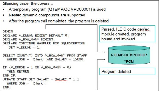
Figure 5-1 Dynamic compound statement implementation
5.2.4 Creating and using global variables
You can use global variables to assign specific variable values for a session. Use the CREATE VARIABLE statement to create a global variable at the server level.
Global variables have a session scope, which means that although they are available to all sessions that are active on the database, their value is private for each session. Modifications to the value of a global variable are not under transaction control. The value of the global variable is preserved when a transaction ends with either a COMMIT or a ROLLBACK statement.
When a global variable is instantiated for a session, changes to the global variable in another session (such as DROP or GRANT) might not affect the variable that is instantiated. An attempt to read from or to write to a global variable created by this statement requires that the authorization ID attempting this action holds the appropriate privilege on the global variable. The definer of the variable is implicitly granted all privileges on the variable.
A created global variable is instantiated to its default value when it is first referenced within its given scope. If a global variable is referenced in a statement, it is instantiated independently of the control flow for that statement.
A global variable is created as a *SRVPGM object. If the variable name is a valid system name but a *SRVPGM exists with that name, an error is generated. If the variable name is not a valid system name, a unique name is generated by using the rules for generating system table names.
If a global variable is created within a session, it cannot be used by other sessions until the unit of work is committed. However, the new global variable can be used within the session that created the variable before the unit of work commits.
Example 5-4 creates a global variable that defines a user class. This variable has its initial value set based on the result of starting a function that is called CLASS_FUNC. This function is assumed to assign a class value, such as administrator or clerk that is based on the USER special register value. The SELECT clause in this example lists all employees from department A00. Only a session that has a global variable with a USER_CLASS value of 1 sees the salaries for these employees.
Example 5-4 Creating and using global variables
CREATE VARIABLE USER_CLASS INT DEFAULT (CLASS_FUNC(USER))
GRANT READ ON VARIABLE USER_CLASS TO PUBLIC
SELECT
EMPNO,
LASTNAME,
CASE
WHEN USER_CLASS = 1
THEN SALARY
ELSE NULL
END
FROM
EMPLOYEE
WHERE
WORKDEPT = 'A00'
5.2.5 Support for arrays in procedures
An array is a structure that contains an ordered collection of data elements in which each element can be referenced by its ordinal position in the collection. If N is the cardinality (number of elements) of an array, the ordinal position that is associated with each element is an integer value greater than or equal to 1 and less than or equal to N. All elements in an array have the same data type.
An array type is a data type that is defined as an array of another data type. Every array type has a maximum cardinality, which is specified on the CREATE TYPE (Array) statement. If A is an array type with maximum cardinality M, the cardinality of a value of type A can be any value 0 - M inclusive. Unlike the maximum cardinality of arrays in programming languages such as C, the maximum cardinality of SQL arrays is not related to their physical representation. Instead, the maximum cardinality is used by the system at run time to ensure that subscripts are within bounds. The amount of memory that is required to represent an array value is proportional to its cardinality, and not to the maximum cardinality of its type.
SQL procedures support parameters and variables of array types. Arrays are a convenient way of passing transient collections of data between an application and a stored procedure or between two stored procedures.
Within SQL stored procedures, arrays can be manipulated as arrays in conventional programming languages. Furthermore, arrays are integrated within the relational model in such a way that data represented as an array can be easily converted into a table, and data in a table column can be aggregated into an array.
Example 5-5 shows two array data types (intArray and stringArray), and a persons table with two columns (ID and name). The processPersons procedure adds three more persons to the table, and returns an array with the person names that contain the letter ‘a’, ordered by ID. The IDs and names of the three persons to be added are represented as two arrays (IDs and names). These arrays are used as arguments to the UNNEST function, which turns the arrays into a two-column table, whose elements are then inserted into the persons table. Finally, the last set statement in the procedure uses the ARRAY_AGG aggregate function to compute the value of the output parameter.
Example 5-5 Support for arrays in procedures
CREATE TYPE intArray AS INTEGER ARRAY[100]
CREATE TYPE stringArray AS VARCHAR(10) ARRAY[100]
CREATE TABLE persons (id INTEGER, name VARCHAR(10))
INSERT INTO persons VALUES(2, 'Tom'),
(4, 'Gina'),
(1, 'Kathy'),
(3, 'John')
CREATE PROCEDURE processPersons(OUT witha stringArray)
BEGIN
DECLARE ids intArray;
DECLARE names stringArray;
SET ids = ARRAY[5,6,7];
SET names = ARRAY['Denise', 'Randy', 'Sue'];
INSERT INTO persons(id, name)
(SELECT t.i, t.n FROM UNNEST(ids, names) AS t(i, n));
SET witha = (SELECT ARRAY_AGG(name ORDER BY id)
FROM persons
WHERE name LIKE '%a%'),
END
If WITH ORDINALITY is specified, an extra counter column of type BIGINT is appended to the temporary table. The ordinality column contains the index position of the elements in the arrays. See Example 5-6.
The ARRAY UNNEST temporary table is an internal data structure and can be created only by the database manager.
Example 5-6 UNNEST temporary table WITH ORDINALITY
CREATE PROCEDURE processCustomers()
BEGIN
DECLARE ids INTEGER ARRAY[100];
DECLARE names VARCHAR(10) ARRAY[100];
set ids = ARRAY[5,6,7];
set names = ARRAY['Ann', 'Bob', 'Sue'];
INSERT INTO customerTable(id, name, order)
(SELECT Customers.id, Customers.name, Customers.order
FROM UNNEST(ids, names) WITH ORDINALITY
AS Customers(id, name, order) );
END
5.2.6 Result set support in embedded SQL
You can write a program in a high-level language (C, RPG, COBOL, and so on) to receive results sets from a stored procedure for either a fixed number of result sets, for which you know the contents, or a variable number of result sets, for which you do not know the contents.
Returning a known number of result sets is simpler. However, if you write the code to handle a varying number of result sets, you do not need to make major modifications to your program if the stored procedure changes.
The basic steps for receiving result sets are as follows:
1. Declare a locator variable for each result set that is returned. If you do not know how many result sets are returned, declare enough result set locators for the maximum number of result sets that might be returned.
2. Call the stored procedure and check the SQL return code. If the SQLCODE from the CALL statement is +466, the stored procedure returned result sets.
3. Determine how many result sets the stored procedure is returning. If you already know how many result sets the stored procedure returns, you can skip this step.
Use the SQL statement DESCRIBE PROCEDURE to determine the number of result sets. The DESCRIBE PROCEDURE places information about the result sets in an SQLDA or
SQL descriptor.
SQL descriptor.
For an SQL descriptor, when the DESCRIBE PROCEDURE statement completes, the following values can be retrieved:
– DB2_RESULT_SETS_COUNT contains the number of result sets returned by the stored procedure.
– One descriptor area item is returned for each result set:
• DB2_CURSOR_NAME
This item contains the name of the cursor that is used by the stored procedure to return the result set.
• DB2_RESULT_SET_ROWS
This item contains the estimated number of rows in the result set. A value of -1 indicates that no estimate of the number of rows in the result set is available.
• DB2_RESULT_SET_LOCATOR
This item contains the value of the result set locator that is associated with the result set.
For an SQLDA, make the SQLDA large enough to hold the maximum number of result sets that the stored procedure might return. When the DESCRIBE PROCEDURE statement completes, the fields in the SQLDA contain the following values:
– SQLDA contains the number of result sets returned by the stored procedure.
– Each SQLVAR entry gives information about a result set. In an SQLVAR entry, the following information is in effect:
• The SQLNAME field contains the name of the cursor that is used by the stored procedure to return the result set.
• The SQLIND field contains the estimated number of rows in the result set. A value of -1 indicates that no estimate of the number of rows in the result set is available.
• The SQLDATA field contains the value of the result set locator, which is the address of the result set.
4. Link result set locators to result sets.
You can use the SQL statement ASSOCIATE LOCATORS to link result set locators to result sets. The ASSOCIATE LOCATORS statement assigns values to the result set locator variables. If you specify more locators than the number of result sets returned, the extra locators are ignored.
If you ran the DESCRIBE PROCEDURE statement previously, the result set locator values can be retrieved from the DB2_RESULT_SET_LOCATOR in the SQL descriptor or from the SQLDATA fields of the SQLDA. You can copy the values from these fields to the result set locator variables manually, or you can run the ASSOCIATE LOCATORS statement to do it for you.
The stored procedure name that you specify in an ASSOCIATE LOCATORS or DESCRIBE PROCEDURE statement must be a procedure name that was used in the CALL statement that returns the result sets.
5. Allocate cursors for fetching rows from the result sets.
Use the SQL statement ALLOCATE CURSOR to link each result set with a cursor. Run one ALLOCATE CURSOR statement for each result set. The cursor names can differ from the cursor names in the stored procedure.
6. Determine the contents of the result sets. If you already know the format of the result set, you can skip this step.
Use the SQL statement DESCRIBE CURSOR to determine the format of a result set and put this information in an SQL descriptor or an SQLDA. For each result set, you need an SQLDA large enough to hold descriptions of all columns in the result set.
You can use DESCRIBE CURSOR only for cursors for which you ran
ALLOCATE CURSOR previously.
ALLOCATE CURSOR previously.
After you run DESCRIBE CURSOR, if the cursor for the result set is declared WITH HOLD, for an SQL descriptor DB2_CURSOR_HOLD can be checked. For an SQLDA, the high-order bit of the eighth byte of field SQLDAID in the SQLDA is set to 1.
Fetch rows from the result sets into host variables by using the cursors that you allocated with the ALLOCATE CURSOR statements. If you ran the DESCRIBE CURSOR statement, complete these steps before you fetch the rows:
a. Allocate storage for host variables and indicator variables. Use the contents of the SQL descriptor or SQLDA from the DESCRIBE CURSOR statement to determine how much storage you need for each host variable.
b. Put the address of the storage for each host variable in the appropriate SQLDATA field of the SQLDA.
c. Put the address of the storage for each indicator variable in the appropriate SQLIND field of the SQLDA.
Fetching rows from a result set is the same as fetching rows from a table.
7. Close the cursors.
Example 5-7 gives you an idea on how to implement this process in an RPG program.
Example 5-7 Result set support in an RPG program
D MYRS1 S SQLTYPE(RESULT_SET_LOCATOR)
D MYRS2 S SQLTYPE(RESULT_SET_LOCATOR)
…
C/EXEC SQL CALL P1(:parm1, :parm2, ...)
C/END-EXEC
…
C/EXEC SQL DESCRIBE PROCEDURE P1 USING DESCRIPTOR :MYRS2
C/END-EXEC
…
C/EXEC SQL ASSOCIATE LOCATORS (:MYRS1,:MYRS2) WITH PROCEDURE P1
C/END-EXEC
C/EXEC SQL ALLOCATE C1 CURSOR FOR RESULT SET :MYRS1
C/END-EXEC
C/EXEC SQL ALLOCATE C2 CURSOR FOR RESULT SET :MYRS2
C/END-EXEC
…
C/EXEC SQL ALLOCATE DESCRIPTOR ‘SQLDES1’
C/END-EXEC
C/EXEC SQL DESCRIBE CURSOR C1 INTO SQL DESCRIPTOR ‘SQLDES1’
C/END-EXEC
5.2.7 FIELDPROC support for encoding and encryption
You can now specify a FIELDPROC attribute for a column, designating an external program name as the field procedure exit routine for that column. It must be an ILE program that does not contain SQL. It cannot be a *SRVPGM, OPM *PGMs, or a Java object. Field procedures are assigned to a table by the FIELDPROC clause of the CREATE TABLE and ALTER TABLE statements. A field procedure is a user-written exit routine that transforms values in a single column.
This procedure allows for transparent encryption / decryption or encoding / decoding of data that is accessed through SQL or any other interface. It allows for transparent encryption or encoding of data that is accessed through SQL or natively.
When values in the column are changed, or new values are inserted, the field procedure is started for each value, and can transform that value (encode it) in any way. The encoded value is then stored. When values are retrieved from the column, the field procedure is started for each value, which is encoded, and must decode it back to the original value. Any indexes that are defined on a non-derived column that uses a field procedure are built with encoded values.
The transformation your field procedure performs on a value is called field-encoding. The same routine is used to undo the transformation when values are retrieved, which is called field-decoding. Values in columns with a field procedure are described to DB2 in two ways:
•The description of the column as defined in CREATE TABLE or ALTER TABLE appears in the catalog table QSYS2.SYSCOLUMNS. This description is the description of the field-decoded value, and is called the column description.
•The description of the encoded value, as it is stored in the database, appears in the catalog table QSYS2.SYSFIELDS. This description is the description of the field-encoded value, and is called the field description.
The field-decoding function must be the exact inverse of the field-encoding function. For example, if a routine encodes ALABAMA to 01, it must decode 01 to ALABAMA. A violation of this rule can lead to unpredictable results.
The field procedure is also started during the processing of the CREATE TABLE or ALTER TABLE statement. That operation is called a field-definition. When so started, the procedure provides DB2 with the column’s field description. The field description defines the data characteristics of the encoded values. By contrast, the information that is supplied for the column in the CREATE TABLE or ALTER TABLE statement defines the data characteristics of the decoded values.
The data type of the encoded value can be any valid SQL data type except ROWID or DATALINK. Also, a field procedure cannot be associated with any column that has values that are generated by IDENTITY or ROW CHANGE TIMESTAMP.
If a DDS-created physical file is altered to add a field procedure, the encoded attribute data type cannot be a LOB type or DataLink. If an SQL table is altered to add a field procedure, the encoded attribute precision field must be 0 if the encoded attribute data type is any of the integer types.
A field procedure cannot be added to a column that has a default value of CURRENT DATE, CURRENT TIME, CURRENT TIMESTAMP, or USER. A column that is defined with a user-defined data type can have a field procedure if the source type of the user-defined data type is any of the allowed SQL data types. DB2 casts the value of the column to the source type before it passes it to the field procedure.
Masking support in FIELDPROCs
FIELDPROCs were originally designed to transparently encode or decode data. Several third-party products use the support in 7.1 to provide transparent column level encryption. For example, to allow a credit card number or social security number to be transparently encrypted on disk.
The FIELDPROC support is extended to allow masking to occur to that same column data (typically based on what user is accessing the data). For example, only users that need to see the actual credit card number see the value, whereas other users might see masked data. For example, XXXX XXXX XXXX 1234.
The new support is enabled by allowing the FIELDPROC program to detect masked data on an update or write operation and returning that indication to the database manager. The database manager then ignores the update of that specific column value on an update operation and replaces it with the default value on a write.
A new parameter is also passed to the FIELDPROC program. For field procedures that mask data, the parameter indicates whether the caller is a system function that requires that the data are decoded without masking. For example, in some cases, RGZPFM and ALTER TABLE might need to copy data. If the field procedure ignores this parameter and masks data when these operations are run, the column data is lost. Hence, it is critical that a field procedure that masks data properly handles this parameter.
Parameter list for execution of field procedures
The field procedure parameter list communicates general information to a field procedure. It signals what operation is to be done and allows the field procedure to signal errors. DB2 provides storage for all parameters that are passed to the field procedure. Therefore, parameters are passed to the field procedure by address.
When you define and use the parameters in the field procedure, ensure that no more storage is referenced for a parameter than is defined for that parameter. The parameters are all stored in the same space and exceeding a parameter’s storage space can overwrite another parameter’s value. This action, in turn, can cause the field procedure to see invalid input data or cause the value returned to the database to be invalid. The following list details the parameters you can pass:
•A 2-byte integer that describes the function to be run. This parameter is input only.
•A structure that defines the field procedure parameter value list (FPPVL).
•The decoded data attribute that is defined by the Column Value Descriptor (CVD). These attributes are the column attributes that were specified at CREATE TABLE or ALTER TABLE time. This parameter is input only.
•The decoded data.
The exact structure depends on the function code.
– If the function code is 8, then the NULL value is used. This parameter is input only.
– If the function code is 0, then the data to be encoded is used. This parameter is input only.
– If the function code is 4, then the location to place the decoded data is used. This parameter is output only.
•The encoded data attribute that is defined by the Field Value Descriptor (FVD). This parameter is input only.
•The encoded data that is defined by the FVD. The exact structure depends on the function code. This parameter is input only.
•The SQLSTATE (character(5)). This parameter is input/output. This parameter is set by DB2 to 00000 before it calls the field procedure. It can be set by the field procedure. Although the SQLSTATE is not normally set by a field procedure, it can be used to signal an error to the database.
•The message text area (varchar(1000)). This parameter is input/output.
5.2.8 Miscellaneous
A number of functions are aggregated under this heading. Most are aimed at upscaling or improving the ease of use for existing functions.
Partitioned table support
A partitioned table is a table where the data is contained in one or more local partitions (members). This release allows you to partition tables that use referential integrity or identity columns.
If you specify a referential constraint where the parent is a partitioned table, the unique index that is used for the unique index that enforces the parent unique constraint must be non-partitioned. Likewise, the identity column cannot be a partitioned key.
Partitioned tables with referential constraints or identity columns cannot be restored to a previous release.
Parameter markers
You can use this function to simplify the definition of variables in a program. Example 5-8 shows how you can write it.
Example 5-8 Parameter markers
SELECT stmt1 =
‘SELECT * FROM t1
WHERE c1 = CAST(? AS DECFLOAT(34)) + CAST(? AS DECFLOAT(34));
PREPARE prestmt1 FROM STMT1;
#Replace this with:
SET STMT1 = ‘SELECT * FROM T1 WHERE C1 > ? + ? ’;
PREPARE PREPSTMT1 FROM STMT;
Expressions in a CALL statement
You can now call a procedure and pass as arguments an expression that does not include an aggregate function or column name. If extended indicator variables are enabled, the extended indicator variable values of DEFAULT and UNASSIGNED must not be used for that expression. In Example 5-9, PARAMETER1 is folded and PARAMETER2 is divided by 100.
Example 5-9 Expressions in a CALL statement
CALL PROC1 ( UPPER(PARAMETER1), PARAMETER2/100 )
Three-part names support
You can use three-part names to bypass the explicit CONNECT or SET CONNECTION. Statements that use three-part names and see distributed data result in IBM DRDA access to the remote relational database. When an application program uses three-part name aliases for remote objects and DRDA access, the application program must be bound at each location that is specified in the three-part names. Also, each alias must be defined at the local site. An alias at a remote site can see yet another server if a referenced alias eventually refers to a table or view.
All object references in a single SQL statement must be in a single relational database. When you create an alias for a table on a remote database, the alias name must be the same as the remote name, but can point to another alias on the remote database. See Example 5-10.
Example 5-10 Three-part alias
CREATE ALIAS shkspr.phl FOR wllm.shkspr.phl
SELECT * FROM shkspr.phl
RDB alias support for 3-part SQL statements
As an alternative to using the CREATE ALIAS SQL statement to deploy database transparency, the Relational Database Directory Entry Alias name can be used instead.
To do this, the SQL statement is coded to refer to the RDB directory entry alias name as the first portion (RDB target) of a 3-part name. By changing the RDB directory entry to have a different destination database using the Remote location (RMTLOCNAME) parameter, the SQL application can target a different database without having to change the application.
Figure 5-2 shows the effect of redefining an RDB alias target.

Figure 5-2 Effect of redefining an RDB alias target
Example 5-11 shows some sample code that pulls daily sales data from different locations.
Example 5-11 Sample code pulling data from different locations
ADDRDBDIRE RDB(X1423P2 MYALIAS) RMTLOCNAME(X1423P2 *IP)
INSERT INTO WORKTABLE SELECT * FROM MYALIAS.SALESLIB.DAILY_SALES
CHGRDBDIRE RDB(LP13UT16 MYALIAS) RMTLOCNAME(LP13UT16 *IP)
INSERT INTO WORKTABLE SELECT * FROM MYALIAS.SALESLIB.DAILY_SALES
Concurrent access resolution
The concurrent access resolution option can be used to minimize transaction wait time. This option directs the database manager how to handle record lock conflicts under certain isolation levels.
The concurrent access resolution option can have one of the following values:
•Wait for outcome
This value is the default. This value directs the database manager to wait for the commit or rollback when it encounters locked data that is being updated or deleted. Locked rows that are being inserted are not skipped. This option does not apply for read-only queries that are running under COMMIT(*NONE) or COMMIT(*CHG).
•Use currently committed
This value allows the database manager to use the currently committed version of the data for read-only queries when it encounters locked data being updated or deleted. Locked rows that are being inserted can be skipped. This option applies where possible when it is running under COMMIT(*CS) and is ignored otherwise. It is what is referred to as “Readers do not block writers and writers do not block readers.”
•Skip locked data
This value directs the database manager to skip rows in the case of record lock conflicts. This option applies only when the query is running under COMMIT(*CS) or COMMIT(*ALL).
The concurrent access resolution values of USE CURRENTLY COMMITTED and SKIP LOCKED DATA can be used to improve concurrency by avoiding lock waits. However, care must be used when you use these options because they might affect application functions.
You can specify the usage for concurrent access resolution in several ways:
•By using the concurrent-access-resolution clause at the statement level for a select-statement, SELECT INTO, searched UPDATE, or searched DELETE
•By using the CONACC keyword on the CRTSQLxxx or RUNSQLSTM commands
•With the CONACC value in the SET OPTION statement
•In the attribute-string of a PREPARE statement
•Using the CREATE or ALTER statement for a FUNCTION, PROCEDURE, or TRIGGER
If the concurrent access resolution option is not directly set by the application, it takes on the value of the SQL_CONCURRENT_ACCESS_RESOLUTION option in the QAQQINI query options file.
CREATE statement
Specifying the CREATE OR REPLACE statement makes it easier to create an object without having to drop it when it exists. This statement can be applied to the following objects:
•ALIAS
•FUNCTION
•PROCEDURE
•SEQUENCE
•TRIGGER
•VARIABLE
•VIEW
To replace an object, the user must have both *OBJEXIST rights to the object and *EXECUTE rights for the schema or library, and privileges to create the object. All existing privileges on the replaced object are preserved.
BIT scalar functions
The bitwise scalar functions BITAND, BITANDNOT, BITOR, BITXOR, and BITNOT operate on the “two’s complement” representation of the integer value of the input arguments. They return the result as a corresponding base 10 integer value in a data type based on the data type of the input arguments. See Table 5-2.
Table 5-2 Bit scalar functions
|
Function
|
Description
|
A bit in the two's complement representation of the result is:
|
|
BITAND
|
Runs a bitwise AND operation.
|
1 only if the corresponding bits in both arguments are 1
|
|
BITANDNOT
|
Clears any bit in the first argument that is in the second argument.
|
Zero if the corresponding bit in the second argument is 1; otherwise, the result is copied from the corresponding bit in the first argument
|
|
BITOR
|
Runs a bitwise OR operation.
|
1 unless the corresponding bits in both arguments are zero
|
|
BITXOR
|
Runs a bitwise exclusive OR operation.
|
1 unless the corresponding bits in both arguments are the same
|
|
BITNOT
|
Runs a bitwise NOT operation.
|
Opposite of the corresponding bit in the argument
|
The arguments must be integer values that are represented by the data types SMALLINT, INTEGER, BIGINT, or DECFLOAT. Arguments of type DECIMAL, REAL, or DOUBLE are cast to DECFLOAT. The value is truncated to a whole number.
The bit manipulation functions can operate on up to 16 bits for SMALLINT, 32 bits for INTEGER, 64 bits for BIGINT, and 113 bits for DECFLOAT. The range of supported DECFLOAT values includes integers -2112 - 2112 -1, and special values such as NaN (Not a Number) or INFINITY are not supported (SQLSTATE 42815). If the two arguments have different data types, the argument that is supporting fewer bits is cast to a value with the data type of the argument that is supporting more bits. This cast affects the bits that are set for negative values. For example, -1 as a SMALLINT value has 16 bits set to 1, which when cast to an INTEGER value has 32 bits set to 1.
The result of the functions with two arguments has the data type of the argument that is highest in the data type precedence list for promotion. If either argument is DECFLOAT, the data type of the result is DECFLOAT(34). If either argument can be null, the result can be null. If either argument is null, the result is the null value.
The result of the BITNOT function has the same data type as the input argument, except that DECIMAL, REAL, DOUBLE, or DECFLOAT(16) returns DECFLOAT(34). If the argument can be null, the result can be null. If the argument is null, the result is the null value.
Because of differences in internal representation between data types and on different hardware platforms, using functions (such as HEX) or host language constructs to view or compare internal representations of BIT function results and arguments is data type dependent and not portable. The data type- and platform-independent way to view or compare BIT function results and arguments is to use the actual integer values.
Use the BITXOR function to toggle bits in a value. Use the BITANDNOT function to clear bits. BITANDNOT(val, pattern) operates more efficiently than BITAND(val, BITNOT(pattern)). Example 5-12 is an example of the result of these operations.
Example 5-12 BIT scalar functions
# Return all items for which the third property bit is set.
SELECT ITEMID FROM ITEM
WHERE BITAND(PROPERTIES, 4) = 4
# Return all items for which the fourth or the sixth property bit is set.
SELECT ITEMID FROM ITEM
WHERE BITAND(PROPERTIES, 40) <> 0
# Clear the twelfth property of the item whose ID is 3412.
UPDATE ITEM
SET PROPERTIES = BITANDNOT(PROPERTIES, 2048)
WHERE ITEMID = 3412
# Set the fifth property of the item whose ID is 3412.
UPDATE ITEM
SET PROPERTIES = BITOR(PROPERTIES, 16)
WHERE ITEMID = 3412
# Toggle the eleventh property of the item whose ID is 3412.
UPDATE ITEM
SET PROPERTIES = BITXOR(PROPERTIES, 1024)
WHERE ITEMID = 3412
# Switch all the bits in a 16-bit value that has only the second bit on.
VALUES BITNOT(CAST(2 AS SMALLINT))
#returns -3 (with a data type of SMALLINT)
Encoded vector index
When you create an encoded vector index (EVI), you can now use an INCLUDE statement in the index option of the CREATE ENCODED VECTOR INDEX command, specifying an aggregate function to be included in the index. These aggregates make it possible for the index to be used directly to return aggregate results for a query. The aggregate function name must be one of the built-in functions AVG, COUNT, COUNT_BIG, SUM, STDDEV, STDDEV_SAMP, VARIANCE, or VARIANCE_SAMP, or a sourced function that is based on one of these built-in functions.
INCLUDE is only allowed for an encoded vector index.
This change has the potential of improving performance on queries that make this type of calculations. Example 5-13 shows the syntax for constructing a simple INCLUDE statement when you create such an index.
Example 5-13 Aggregate function support for EVI
CREATE ENCODED VECTOR INDEX GLDSTRN.RSNKRNZ_EVI1
ON GLDSTRN.HMLT (JOB_TYPE, JOB_CATEGORY)
INCLUDE (AVG(WORK_TIME))
Inlining of scalar functions
In cases of simple SQL scalar functions, instead of starting the function as part of a query, the expression in the RETURN statement of the function can be copied (inlined) into the query itself. Such a function is called an inline function. A function is an inline function if the following criteria are met:
•The SQL function is deterministic.
•The SQL-routine-body contains only a RETURN statement.
•The RETURN statement does not contain a scalar subselect or fullselect.
INSERT with remote SUBSELECT
INSERT with SUBSELECT is enhanced to allow the select to reference a single remote database that is different from the current server connection
An implicit remote connection is established and used by DB2 for i.
This enhancement is the second installment in extending DB2 for i on 7.1 to use implicit or explicit remote three-part names within SQL.
Example 5-14 declares the global temporary table from a remote subselect, which is followed by the insert.
Example 5-14 Usage of INSERT with remote SUBSELECT
DECLARE GLOBAL TEMPORARY TABLE SESSION.MY_TEMP_TABLE (SERVER_NAME VARCHAR(40), DATA_VALUE CHAR(1)) WITH REPLACE
INSERT INTO SESSION.MY_TEMP_TABLE (SELECT CURRENT_SERVER CONCAT ‘is the server name’, IBMREQD FROM EUT72P1.SYSIBM.SYSDUMMY1)
SELECT * FROM SESSION.MY_TEMP_TABLE;
Figure 5-3 displays the output that is generated from Example 5-14 on page 181.
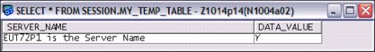
Figure 5-3 Clearly showing the result was from a remote subselect
SQL procedure and function obfuscation
Obfuscation provides the capability of optionally obscuring proprietary SQL statements and logic within SQL procedures or functions.
ISVs can use this support to prevent their customers from seeing or changing SQL routines that are delivered as part of their solution.
Example 5-15 demonstrates how obfuscation is performed.
Example 5-15 Example of obfuscation
CALL SYSIBMADM.CREATE_WRAPPED('CREATE PROCEDURE UPDATE_STAFF (
IN P_EmpNo CHAR(6),
IN P_NewJob CHAR(5),
IN P_Dept INTEGER)
LANGUAGE SQL
TR : BEGIN
UPDATE STAFF
SET JOB = P_NewJob
WHERE DEPT = P_Dept and ID = P_EmpNo; END TR '),
SELECT ROUTINE_DEFINITION FROM QSYS2.SYSROUTINE WHERE
ROUTINE_NAME = 'UPDATE_STAFF';
The output in Figure 5-4 clearly shows the result of obfuscation.
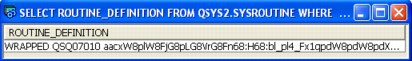
Figure 5-4 Output of routine clearly showing obfuscation
System i Navigator can also be used to obfuscate SQL through the Generate SQL option by selecting Obfuscate (for SQL function, and procedures) as shown in Figure 5-5.
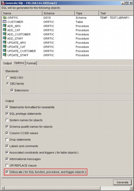
Figure 5-5 Obfuscate (for SQL function and procedure objects) check box
Figure 5-6 shows an example of obfuscated code after the option to obfuscate is selected.
|
Important: The obfuscate option is not available for triggers.
|
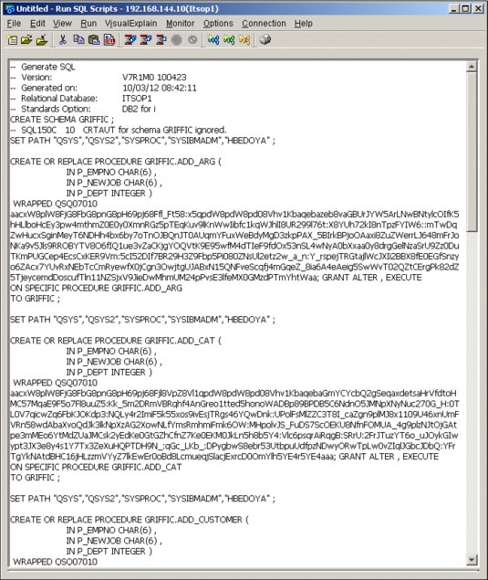
Figure 5-6 Example of obfuscated code
CREATE TABLE with remote SUBSELECT
One of the enhancements in the CREATE TABLE command in IBM i 7.1 is the capability of creating a table based on a remote table.
•CREATE TABLE AS and DECLARE GLOBAL TEMPORARY TABLE are enhanced to allow the select to reference a single remote database that is different from the current server connection.
•An implicit remote connection is established and used by DB2 for i.
•The remote query can reference a single remote homogeneous or heterogeneous table.
This enhancement is the third installment for extending DB2 for i on 7.1 to use implicit or explicit remote three-part names within SQL.
A table is created based on a remote table, as shown in Example 5-16.
Example 5-16 Create a table in the local database that references a remote database with the AS clause
CREATE TABLE DATALIB.MY_TEMP_TABLE AS (SELECT CURRENT_SERVER CONCAT ' is the Server Name', IBMREQD
FROM X1423P2.SYSIBM.SYSDUMMY1) WITH DATA
SELECT * FROM DATALIB.MY_TEMP_TABLE
Running the example SQL produces the output that shows that a remote table was accessed, as shown in Figure 5-7.

Figure 5-7 Output from the SQL showing that the remote table was accessed
5.2.9 Generating field reference detail on CREATE TABLE AS
Impact Analysis tools use reference field information to identify tables and programs that need to be modified. Before this enhancement, SQL tables did not propagate reference information.
CREATE TABLE AS is enhanced to store the originating column and table as the reference information in the file object.
When using LIKE to copy columns from another table, REFFLD information is copied for each column that has a REFFLD in the original table.
When using AS to define a new column, any column that directly references a table or view (not used in an expression) has a REFFLD defined that refers to that column. A simple CAST also generates REFFLD information (that is, CAST (PARTNAME as varchar(50)))
As an example, if the following table is created:
create table slr/base (a int, b int, c int)
create table slr/as1 as (select * from slr/base) with no data
create table slr/like1 like slr/as1
The improved field reference detail is as shown in Figure 5-8.
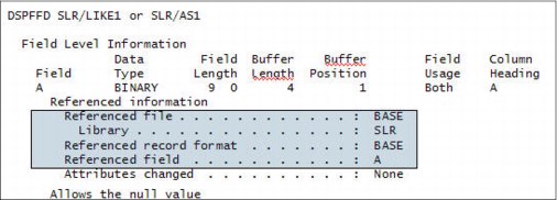
Figure 5-8 CREATE TABLE AS field reference detail
5.2.10 Qualified name option added to generate SQL
Today, generated SQL includes schema/library qualification of objects.
System i Navigator and the QSQGNDDL() are enhanced to include the qualified name option, making it easier to redeploy generated SQL. Any three-part names (object and column) are left unchanged. Any schema qualification within the object that does not match the database object library name are left unchanged.
The qualified name option specifies whether qualified or unqualified names should be generated for the specified database object. The valid values are:
‘0’ Qualified object names should be generated. Unqualified names within the body of SQL routines remain unqualified (by default).
‘1’ Unqualified object names should be generated when a library is found that matches the database object library name. Any SQL object or column reference that is RDB qualified is generated in its fully qualified form. For example, rdb-name.schema-name.table-name and rdb-name.schema-name.table-name.column-name references retain their full qualification. This option also appears on the Generate SQL dialog within System i Navigator, as shown in Figure 5-9 on page 187. The default behavior is to continue to generate SQL with schema qualification.

Figure 5-9 Schema qualified names for objects check box
5.2.11 New generate SQL option for modernization
Today, an SQL view is generated for DDS-created keyed physical, keyed logical, or join logical files. With this enhancement, IBM i Navigator has more generate SQL options. The options are mutually exclusive options and have been added to QSQGNDDL and IBM i Navigator.
This enhancement makes it easier to proceed with DDS to SQL DDL modernization.
The following examples provide samples of the new generate SQL option for modernization. There is a generate additional indexes option for keyed physical and logical files whether more CREATE INDEX statements are generated for DDS created keyed physical, keyed logical, or join logical files.
Example 5-17 shows a sample DDS for join logical file.
Example 5-17 Sample DDS for a join logical file
R FMT JFILE(MJATST/GT MJATST/GT2)
J JFLD(F1_5A F1_5A)
F1_5A JREF(1)
F2_5A JREF(2)
K F1_5A
The resulting v statement after using the generate SQL for modernization option is shown in Example 5-18.
Example 5-18 Resulting CREATE VIEW statement after using Generate SQL for modernization option
CREATE VIEW MJATST.GVJ (
F1_5A , F2_5A )
AS
SELECT
Q01.F1_5A , Q02.F2_5A
FROM MJATST.GT AS Q01 INNER JOIN
MJATST.GT2 AS Q02 ON ( Q01.F1_5A = Q02.F1_5A )
RCDFMT FMT;
CREATE INDEX MJATST.GVJ_QSQGNDDL_00001
ON MJATST.GT ( F1_5A ASC );
CREATE INDEX MJATST.GVJ_QSQGNDDL_00002
ON MJATST.GT2 ( F1_5A ASC );
There is also a generate index instead of view option, which specifies whether a CREATE INDEX or CREATE VIEW statement is generated for a DDS-created keyed logical file. Example 5-19 shows the DDS created keyed logical file.
Example 5-19 DDS created keyed logical file
R FMT PFILE(MJATST/GT)
F3_10A
F2_5A
F1_5A
K F3_10A
Example 5-20 shows the resulting CREATE INDEX statement
Example 5-20 Resulting CREATE INDEX statement
CREATE INDEX MJATST.GV2
ON MJATST.GT ( F3_10A ASC )
RCDFMT FMT;
5.2.12 OVRDBF SEQONLY(YES, buffer length)
OVRDBF adds support to allow the user to specify the buffer length rather than the number of records for OVRDBF SEQONLY(*YES N). N can be:
•*BUF32KB
•*BUF64KB
•*BUF128KB
•*BUF256KB
This setting means that the number of records are the number of records that fit into a 32 KB,
64 KB, 128 KB, or 256 KB buffer.
64 KB, 128 KB, or 256 KB buffer.
5.3 Performance and query optimization
In the IBM i 7.1 release of DB2 for i, a considerable effort was undertaken to enhance the runtime performance of the database, either by extending existing functions or by introducing new mechanisms.
Runtime performance is affected by many issues, such as the database design (the entity-relationship model, which is a conceptual schema or semantic data model of a relational database), the redundancy between functional environments in composite application environment, the level of normalization, and the size and volumes processed. All of these items influence the run time, throughput, or response time, which is supported by the IT components and is defined by the needs of the business. Performance optimization for database access must address all the components that are used in obtained acceptable and sustainable results, covering the functional aspects and the technical components that support them.
This section describes the query optimization method. It describes what is behind the changes that are implemented in the database management components to relieve the burden that is associated with the tools and processes a database administrator uses or follows to realize the non-functional requirements about performance and scalability. These requirements include the following:
•Global Statistics Cache (GSC)
•Adaptive Query Processing
•Sparse indexes
•Encoded vector index-only access, symbol table scan, symbol table probe, and
INCLUDE aggregates
INCLUDE aggregates
•Keeping tables or indexes in memory
5.3.1 Methods and tools for performance optimization
Typically, the autonomous functions in IBM i, and the new ones in IBM i 7.1, all strive to obtain the best possible performance and throughput. However, you can tweak settings to pre-emptively enhance the tooling of IBM i.
In today’s business world, the dynamics of a business environment demand quick adaptation to changes. You might face issues by using a too generic approach in using these facilities. Consider that you made the architectural decision for a new application to use a stateless runtime environment and that your detailed component model has the infrastructure for it. If the business processes it supports are changing and require a more stateful design, you might face an issue if you want to preserve information to track the statefulness in your transactions. Then, the database where you store information about these transactions might quickly become the heaviest consumer of I/O operations. If your infrastructure model did not consider this factor, you have a serious issue. Having high volumes with a low latency is good. However, this situation must be balanced against the effort it takes to make it sustainable and manageable throughout all of the IT components you need to support the business.
When you define components for a database support, develop a methodology and use preferred practices to obtain the best results. Any methodology must be consistent, acceptable, measurable, and sustainable. You want to stay away from ad hoc measures or simple bypasses.
IBM i provides statistics about I/O operations, provided by the database management function. These statistics show accumulated values, from which you can derive averages, on the I/O operations on tables and indexes. These statistics do not take into account the variability and the dynamic nature of the business functions these objects support. So if you want to use these statistics to define those objects to be placed either in memory or on faster disks, you must consider a larger scope.
For example: Since the introduction of solid-state drives (SSD), which have a low latency, the IBM i storage manager has awareness about this technology and uses it as appropriate. Since release 6.1, you can specify the media preference on the CREATE TABLE/INDEX and ALTER TABLE/INDEX commands along with the DECLARE GLOBAL TEMPORARY TABLE (see 5.3.9, “SQE optimization for indexes on SSD” on page 196). The SYSTABLESTAT and SYSINDEXSTAT catalog tables provide more I/O statistics (SEQUENTIAL_READS and RANDOM_READS) in release 7.1 on these objects. These statistics, generated by the database manager, indicate only possible candidates to be housed on SSD hardware. Further investigation of the run time and the contribution to the performance and capacity or the infrastructure reveals whether they are eligible for those settings.
For more information about SSDs, see Chapter 8, “Storage and solid-state drives” on page 377.
Finally, and as a last resort, there is now a stored procedure available that you can use to cancel long running SQL jobs using the QSYS2.CANCEL_SQL procedure.
5.3.2 Query optimization
Whenever a query is submitted, the database engine creates an artifact that allows the query to trigger a set of events and processes that allows it to run the request with the lowest cost. In this context, cost is expressed as the shortest time possible to run the query. This cost calculation is done on a number of both fixed and variable elements. The fixed cost elements are attributes, such as both the hardware components (processor, memory, and disks) and in the instruments or methods that can be used to handle rows and columns in a (set of) database files. These methods are known as using indexes (binary radix index or encoded vector index), index or table scan, hashing, sorting, and so on. The variable elements are typically the volume of data (that is, the number or rows) to be handled and the join functions that are required by the query. Based on these methods, the database query engine builds an access plan that targets reduction of cost.
Even with all the technologies that are used, the access plans might still yield an incorrect (that is, not obeying the rule of capping the cost) result. This situation can, for example, be the result of not having an index to navigate correctly through the data. For that reason, IBM i supports the technology to create temporary indexes autonomically until the system undergoes an IPL. This index can be used by any query that might benefit from its existence. These autonomous indexes can be viewed and carry information that a database administrator can use to decide whether to make it a permanent object by using the definition of the temporary index.
Other elements that can contribute to incorrect access plans are as follows:
•Inclusion of complex or derivated predicates, which are hard to predict without running the query about the existence of stale statistics on busy systems
•Hidden correlations in the data, often because of a poor design, data skew, and data volatility
•Changes in the business or infrastructure environment
In the last case, this situation is more likely to happen with variations in both memory and processor allocations on partitioned systems, which are reconfigured using dynamic partitioning. It can also be caused when the data is changed frequently in bulk.
If you want to read more about the database query engine, see Preparing for and Tuning the SQL Query Engine on DB2 for i5/OS, SG24-6598.
5.3.3 Global statistics cache
There are several process models to reduce the impact of managing the dynamics of a database structure and its content. Moreover, this database is often deployed on a system that is subject to many changes. These tasks can be a wide array of non-automated interventions, including the setup of a validation process of access plans, manually tuning the query, or having the access plans invalidated and re-created. It can also include a reset of the statistics information or an extensive review of the query functions to achieve a higher degree of expected consumability by the system. These actions are typically post-mortem actions and are labor-intensive.
To reduce this labor-intensive work, the DB2 Statistics Manager was revised. By default, it now collects data about observed statistics in the database and from partially or fully completed queries. This data is stored in the Global Statistics Cache (GSC), which is a system-wide repository, containing those complex statistics. The adaptive query processing (AQP) (see 5.3.4, “Adaptive query processing” on page 192) inspects the results of queries and compares the estimated row counts with the actual row counts. All of the queries that are processed by the SQL Query Engine (SQE) use this information to increase overall efficiency. One of the typical actions the SQE can take is to use the live statistics in the GSC, compare the estimated row count with the actual row count, and reoptimize and restart the query using the new query plan. Furthermore, if another query asks for the same or a similar row count, the Storage Manager (SM) can return the stored actual row count from the GSC. This action allows generating faster query plans by the query optimizer.
Typically, observed statistics are for complex predicates, such as a join. A simple example is a query that joins three files, A, B, and C. There is a discrepancy between the estimate and actual row count of the join of A and B. The SM stores an observed statistic into the GSC. Later, if a join query of A, B, and Z is submitted, SM recalls the observed statistic of the A and B join. The SM considers that observed statistic in its estimate of the A, B, and Z join.
The GSC is an internal DB2 object, and the contents of it are not directly observable. You can harvest the I/O statistics in the database catalog tables SYSTABLESTAT and SYSINDEXSTAT or by looking at the I/O statistics using the Display File Description (DSPFD) command. This command provides only a limited number of I/O operations. Both counters (catalog tables and the object description) are reset at IPL time.
The statistics collection is defined by the system value Data Base file statistics collection (QDBFSTCCOL). The SM jobs that update the statistics carry the same name.
5.3.4 Adaptive query processing
The SQE uses statistics to build the mechanism to run an SQL statement. These statistics come from two sources:
•Information that is contained in the indexes on the tables that are used in the statement
•Information that is contained in the statistics tables (the GSC)
When the query compiler optimizes the query plans, its decisions are heavily influenced by statistical information about the size of the database tables, indexes, and statistical views. The optimizer also uses information about the distribution of data in specific columns of tables, indexes, and statistical views if these columns are used to select rows or join tables. The optimizer uses this information to estimate the costs of alternative access plans for each query.
In IBM i 7.1, the SQE query engine uses a technique called adaptive query processing (AQP). AQP analyzes actual query runtime statistics and uses that information to correct previous estimates. These updated estimates can provide better information for subsequent optimizations. It also focuses on optimizing join statements to improve the join orders and minimizing the creation of large dials for sparsely populated join results. This inspection is done during the run of a query request and observes its progress. The AQP handler wakes up after a query runs for at least 2 seconds without returning any rows. Its mission is to analyze the actual statistics from the partial query run, diagnose, and possibly recover from join order problems. These join order problems are because of inaccurate statistical estimates. This process is referred to as the AQP Handler.
After a query completes, another task, the AQP Request Support, starts and runs in a system task so that it does not affect the performance of user applications. Estimated record counts are compared to the actual values. If significant discrepancies are noted, the AQP Request Support stores the observed statistic in the GSC. The AQP Request Support might also make specific recommendations for improving the query plan the next time the query runs.
Both tasks collect enough information to reoptimize the query using partially observed statistics or specific join order recommendations or both. If this optimization results in a new plan, the old plan is stopped and the query is restarted with the new plan, provided that the query has not returned any results. The restart can be done for long running queries during the run time itself.
AQP looks for an unexpected starvation join condition when it analyzes join performance. Starvation join is a condition where a table late in the join order eliminates many records from the result set. In general, the query can run better if the table that eliminates the large number of rows is first in the join order. When AQP identifies a table that causes an unexpected starvation join condition, the table is noted as the forced primary table. The forced primary table is saved for a subsequent optimization of the query. That optimization with the forced primary recommendation can be used in two ways:
•The forced primary table is placed first in the join order, overriding the join order that is implied by the statistical estimates. The rest of the join order is defined by using existing techniques.
•The forced primary table can be used for LPG preselection against a large fact table in the join.
The database monitor has a new set of records to identify the action that is undertaken with by the AQP.
Figure 5-10 provides a sample of how a join can be optimized. The estimated return of rows on table C proved to be much smaller during the execution of the query, forcing the SQE to recalculate the number of rows that are returned and dramatically reduced the size of the result set.
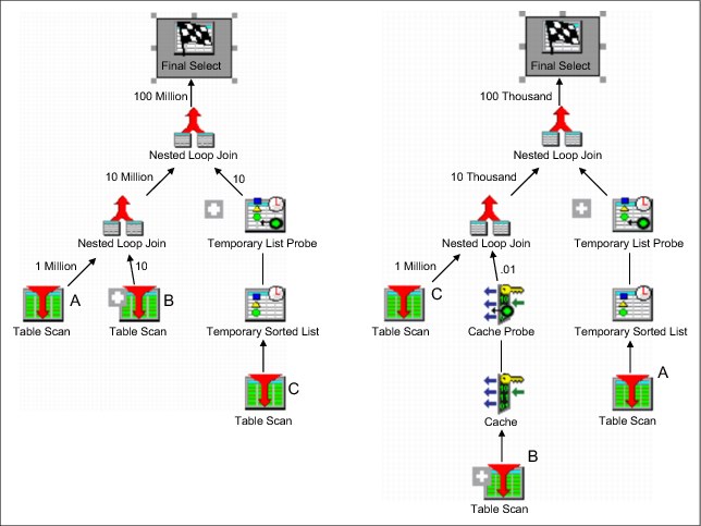
Figure 5-10 AQP Optimization on join
5.3.5 Sparse indexes
Starting from the IBM i 6.1 release, you can create a sparse index by using a WHERE condition. In IBM i 7.1, the query optimizer inspects those indexes and uses them where appropriate.
The reason for creating a sparse index is to provide performance enhancements for your queries. The performance enhancement is done by precomputing and storing results of the WHERE selection in the sparse index. The database engine can use these results instead of recomputing them for a user-specified query. The query optimizer looks for any applicable sparse index and can choose to implement the query by using a sparse index. The decision is based on whether using a sparse index is a faster implementation choice.
To use a sparse index, the WHERE selection in the query must be a subset of the WHERE selection in the sparse index. The set of records in the sparse index must contain all the records to be selected by the query. It might contain additional records. This comparison of the WHERE selection is performed by the query optimizer during optimization. It is like the comparison that is run for Materialized Query Tables (MQT).
Besides the comparison of the WHERE selection, the optimization of a sparse index is identical to the optimization that is run for any Binary Radix index.
Example 5-21 shows creating a sparse index over a table in which events are stored. These events can be of four types:
•On-stage shows (type OSS)
•Movies (type MOV)
•Broadcasts (BRO)
•Forums (FOR)
Example 5-21 Sparse indexes
CREATE INDEX EVENTS/OSS_MOV_BRO on EVENTS/OSS_MOV_BRO_FOR (EVTYPE)
WHERE EVTYPE in (‘OSS’, ‘MOV’, BRO’);
CREATE INDEX EVENTS/OSS_MOV_BRO_FOR on EVENTS/OSS_MOV_BRO_FOR (EVTYPE)
WHERE EVTYPE in (‘OSS’, ‘MOV’, BRO’, ‘FOR’);
In the first index, select type OSS, MOV, and BRO, and in the second index, all of the types. In the first index, the query selection is a subset of the sparse index selection and an index scan over the sparse index is used. The remaining query selection (EVTYPE=FOR) is run following the index scan. For the second index, the query selection is not a subset of the sparse index selection and the sparse index cannot be used.
5.3.6 Encoded vector index
Section “Encoded vector index” on page 181 described the enhancements for encoded vector indexes (EVIs). The EVI can be used for more than generating a bitmap or row number list to provide an asynchronous I/O map to the wanted table rows. The EVI can also be used by two index-only access methods that can be applied specifically to the symbol table itself. These two index-only access methods are the EVI symbol table scan and the EVI symbol table probe.
These two methods can be used with GROUP BY or DISTINCT queries that can be satisfied by the symbol table. This symbol table-only access can be further employed in aggregate queries by adding INCLUDE values to the encoded vector index.
EVI symbol table scan
An encoded vector index symbol table scan operation is used to retrieve the entries from the symbol table portion of the index. All entries (symbols) in the symbol table are sequentially scanned if a scan is chosen. The symbol table can be used by the optimizer to satisfy GROUP BY or DISTINCT portions of a query request.
Selection is applied to every entry in the symbol table. The selection must be applied to the symbol table keys unless the EVI was created as a sparse index with a WHERE clause. In that case, a portion of the selection is applied as the symbol table is built and maintained. The query request must include matching predicates to use the sparse EVI.
All entries are retrieved directly from the symbol table portion of the index without any access to the vector portion of the index. There is also no access to the records in the associated table over which the EVI is built.
The advantages of this setup are obvious:
•Pre-summarized results are readily available.
•There is a need to process only the unique values in the symbol table, thus avoiding processing table records.
•It extracts all the data from the index unique key values or INCLUDE values, thus eliminating the need for a Table Probe or vector scan.
•With INCLUDE providing ready-made numeric aggregates, it eliminates the need to access corresponding table rows to run the aggregation.
However, for grouping queries where the resulting number of groups is relatively small compared to the number of records in the underlying table, the performance improvement is low. Even more, it can perform poorly when many groups are involved, making the symbol table large. You are likely to experience poor performance if a large portion of the symbol table is put into the overflow area. Alternatively, you experience a significant performance improvement for grouping queries when the aggregate is specified as an INCLUDE value of the symbol table.
INCLUDE aggregates
To enhance the ability of the EVI symbol table to provide aggregate answers, the symbol table can be created to contain more INCLUDE values. These results are ready-made numeric aggregate results, such as SUM, COUNT, AVG, or VARIANCE values that are requested over non-key data. These aggregates are specified using the INCLUDE keyword on the CREATE ENCODED VECTOR INDEX request.
These included aggregates are maintained in real time as rows are inserted, updated, or deleted from the corresponding table. The symbol table maintains these additional aggregate values in addition to the EVI keys for each symbol table entry. Because these results are numeric results and finite in size, the symbol table is still a desirable compact size.
The included aggregates are over non-key columns in the table where the grouping is over the corresponding EVI symbol table defined keys. The aggregate can be over a single column or a derivation.
Encoded vector index symbol table probe
The encoded vector index symbol table probe operation is used to retrieve entries from the symbol table portion of the index, which avoids scanning the entire symbol table. The symbol table can be used by the optimizer to satisfy GROUP BY or DISTINCT portions of a query request.
The optimizer attempts to match the columns that are used for the selection against the leading keys of the EVI index. It then rewrites the selection into a series of ranges that can be used to probe directly into the symbol table. Only those symbol table pages from the series of ranges are paged into main memory. The resulting symbol table entries that are generated by the probe operation can then be further processed by any remaining selection against EVI keys. This strategy provides for quick access to only the entries of the symbol table that satisfy the selection.
Similar to an encoded vector symbol table scan, a symbol table probe can return ready-made aggregate results if INCLUDE is specified when the EVI is created. All entries are retrieved directly from the symbol table portion of the index without any access to the vector portion of the index. In addition, it is unnecessary to access the records in the associated table over which the EVI is built.
5.3.7 Preserving EVI indexes on ALTER enhancement
Before this enhancement, an ALTER TABLE or fast delete under commitment control required any encoded vector indexes on the table to be altered to be rebuilt.
This enhancement allows encoded vector indexes on the table being altered to be preserved if the data type or other attribute of a key column of the index is not changed by the ALTER.
5.3.8 Keeping tables or indexes in memory
The KEEPINMEM parameter specifies whether the data or an access for a file member is brought into a main storage pool by the SQL Query Engine (SQE) when the data is used in the query to improve the performance. When you specify *YES for this parameter, the Query Options File (QAQQINI) parameter MEMORY_POOL_PREFERENCE (see 5.3.17, “QAQQINI properties” on page 200) specifies the preferred main storage pool to be used.
This function applies only during the run time of a query, and might therefore be substituted for the Set Object Access (SETOBJACC) command that puts the table or index in memory in a static function. After the query completes, the memory might be freed again, contrary to the effects of the Set Object Access (SETOBJACC), where you must clear it using the *PURGE option on the Storage Pool (POOL) parameter of the command.
Similarly, the DB2 database manager reduces the amount of storage that is occupied by a table that does not contain any data. This reduces the storage space that is needed for unused objects. This situation is also referred to as deflated table support.
5.3.9 SQE optimization for indexes on SSD
The query optimizer now recognizes that indexes might potentially be on SSDs and prioritizes usage of those indexes higher than indexes on spinning disk when you order the indexes during optimization.
Indexes must have the SSD attribute specified through the UNIT(*SSD) parameter on the Create Logical File (CRTLF) or Change Logical File (CHGLF) CL commands, or by using the UNIT SSD clause on the SQL CREATE INDEX statement. For more information, see 5.4.11, “CHGPFM and CHGLFM UNIT support” on page 221.
5.3.10 SQE support of simple logical files
SQE supports simple logical files in IBM i 7.1. SQE support of simple logical files has the following restrictions:
•No SQE support of OmniFind using logical files.
•No SQE support of multi-data space logical files.
•No SQE support of logical files over a partition table.
•SQE supports only read-only queries. There is no SQE support of insert, update, or delete using logical files.
The QAQQINI file option 'IGNORE_DERIVED_INDEX' continues to be supported. If IGNORE_DERIVED_INDEX(*NO) is specified, and a select / omit logical file exists based on file of the simple logical file, then SQE does not process the query of the simple logical file.
5.3.11 Maximum size of an SQL index increased to 1.7 TB
The maximum size of an SQL index has been increased to 1.7 TB. Few indexes approach 1 TB today. However, this enhancement extends an important limit for Very Large Database (VLDB) considerations. See Figure 5-11.

Figure 5-11 Very large index limit increasing to 1.7 TB
5.3.12 QSYS2.INDEX_ADVICE procedure
This procedure is useful to anyone who wants to analyze index advice from different systems or from different points in time.
The DB2 for i index advice condenser is externalized through the QSYS2.CONDENSEDINDEXADVICE view. The view and underlying user-defined table function are hardwired to use the raw index advice that is stored within the QSYS2/SYSIXADV file. Some users must use the index advice condenser against a file that was saved and restored from a different system.
A new database supplied procedure (QSYS2.INDEX_ADVICE) was added. The procedure establishes the QTEMP/CONDENSEDINDEXADVICE view over a user supplied library and file name. After this is established, the user can query QTEMP/CONDENSEDINDEXADVICE to condense the index advice against the target index advice file.
The QSYS2.INDEX_ADVICE procedure also has options to return the index advice as a result set, either in raw advice format or in condensed format. When the job ends or disconnects, the objects in QTEMP are automatically removed. The QSYS2.INDEX_ADVICE procedure also has options to return the index advice as a result set, either in raw advice format or in condensed format.
Example 5-22 illustrates the usage of the INDEX_ADVISE procedure.
Example 5-22 Usage of QSYS2.INDEX_ADVICE procedure
#Procedure definition:
create procedure QSYS2.INDEX_ADVICE(
in advice_library_name char(10),
in advice_file_name char(10),
in advice_option integer)
in advice_library_name char(10),
in advice_file_name char(10),
in advice_option integer)
#Advice_option values:
#if advice_option=0 then setup for targeted condensed index advice, do not return a result set
#if advice_option=1 return condensed index advice as a result set
#if advice_option=2 return raw index advice as a result set
#Example usage:
#if advice_option=1 return condensed index advice as a result set
#if advice_option=2 return raw index advice as a result set
#Example usage:
call qsys2.index_advice('ADVICELIB', 'SYSIXADV', 0);
-- Count the rows of raw advice
select count(*) from QTEMP.SYSIXADV where table_schema = 'PRODLIB' ;
select count(*) from QTEMP.SYSIXADV where table_schema = 'PRODLIB' ;
-- Count the rows of condensed advice
select count(*) from QTEMP.CONDENSEDINDEXADVICE where table_schema = 'PRODLIB';
-- Review an overview of the most frequently advised, using condensed advice
select table_name, times_advised, key_columns_advised from QTEMP.CONDENSEDINDEXADVICE where table_schema = 'PRODLIB' order by times_advised desc;
When the procedure is called with advice_option=0, the index advice level of the target file is determined. If the advice file originated from an IBM i 5.4 or 6.1 system, the file is altered to match the 7.1 advice format. This alteration is a one time conversion of the advice file. After this is established, the user can query QTEMP.CONDENSEDINDEXADVICE to condense the index advice against the target index advice file.
5.3.13 Improved index advice generation to handle OR predicates
Index Advisor has been extended for include queries which OR together local selection (WHERE clause) columns over a single table. OR advice requires two or more indexes to be created as a set.
If any of the OR'ed indexes are missing, the optimizer is not able to use the indexes for implementation of the OR-based query. This relationship is surfaced within the QSYS2/SYSIXADV index advice table within a new DEPENDENT_ADVICE_COUNT column.
This column has a data type of BIGINT and the column value means the following:
•Zero: This advised index stands on its own, no OR selection.
•Greater than zero: Compare this column against the TIMES_ADVISED column to understand how often this advised index has both OR and non-OR selection. Dependent implies it depends on other advised indexes and all of the advised indexes must exist for a bitmap implementation to be used
When Index Advisor shows highly dependent advice, use the Exact Match capability from Show Statements to find the query in the plan cache. Additional information about the exact match capability can be found on the following website:
After it is found, use Visual Explain to discover the dependent index advice specific to that query. Some restrictions with this support are as follows:
•OR'ed predicate advice appears only if no other advice is generated
•Maximum of five predicates OR'ed together
•Advised for files with OR'd local selection that gets costed in the primary (first) join dial when optimizing a join query
Example 5-23 shows advise indexes over all three OR’ed predicate columns. Also, all three advised indexes have DEPENDENT_ADVICE_COUNT > 0.
Example 5-23 Index OR Advice example
select orderkey, partkey, suppkey,
linenumber, shipmode orderpriority
from ABC_ITEM_fact
where OrderKey <= 10 OR
SuppKey <= 10 OR
PartKey <= 10
optimize for all rows
Figure 5-12 shows the execution of the query with the advised indexes and no new advice are registered.

Figure 5-12 Index advice for OR predicate
5.3.14 SKIP LOCKED DATA and NC or UR
You can use the SKIP LOCKED DATA clause to fetch rows from a table or view without waiting for row locks. When the option is specified, any row that is already locked by another job is skipped. This behavior is typically wanted for tables or views that are used as a queue. SKIP LOCKED DATA can be used only when isolation level NC, UR, CS, or RS is in effect. The SKIP LOCKED DATA clause is ignored when used when isolation level RR is in effect.
Before this enhancement, SKIP LOCKED DATA was allowed only when the isolation level was CS or RS.
For more information about this topic, go to:
5.3.15 SQL routine performance integer arithmetic (requires re-create)
This procedure improves the performance of the generated code within LANGUAGE SQL routines. When you add and subtract a positive integer from an SQL smallint, integer, and bigint variable in a LANGUAGE SQL procedure, function, or trigger, the assignment is accomplished directly within the generated ILE C code. This improvement is not observed when you build SQL routines for previous releases (for example, when you use SET OPTION TGTRLS=V6R1M0 or V5R4M0).
To achieve the improved code generation, SQL procedures, functions, and trigger routines must be re-created after you upgrade the operating system to IBM i 7.1.
This improvement applies to the following usage of the SQL SET statement:
SET v1 = v1 + <in lit> where v1 is a smallint, in, and bigint
SET v1 = v1 - <in lit> where v1 is a smallint, in, and bigint
The following statements will generate inline ILE C code:
SET v1 = v1 + <integer literal>
SET v1 = v1 + <bigint literal>
SET v1 = v1 + <negative integer literal>
SET v1 = v1 + <integer literal>
SET v1 = v1 + <bigint literal>
SET v1 = v1 + <negative integer literal>
SET v1 = <any literal> + v1
SET v1 = <any literal> +/- <any literal>
SET v1 = <any literal> +/- <any literal>
These statements do not generate inline ILE C code:
SET v1 = v2 + <integer literal>
SET v2 = v1 + <bigint literal>
SET v2 = v1 + <bigint literal>
5.3.16 Automatic cancellation of QSQSRVR jobs when an application ends
When an application using SQL Server Mode is stopped and the SQL Server Mode connections are not ended, the termination of the application job might completely end while the QSQSRVR job remains active running a long running system operation.
Job termination is improved to signal an SQL Cancel request to any QSQSRVR jobs that being used by the application. The cancellation interrupts some long running operations, allowing the QSQSRVR job to observe that the application is ending.
SQL Server Mode users must apply only the PTF to receive the improved cancel handling support.
5.3.17 QAQQINI properties
Table 5-3 lists the new parameters and their values that can be put in the QAQQINI file, which is used to define settings for processes that run queries. These changes are in line with the new features in the DB2 for i.
Table 5-3 QAQQINI file
|
Parameter
|
Description
|
|
ALLOW_ADAPTIVE_QUERY_PROCESSING
(For more information, see 5.3.4, “Adaptive query processing” on page 192.)
|
Specifies whether AQP processing is done for a query.
|
|
ALLOW_ARRAY_VALUE_CHANGES
|
Specifies whether changes to the values of array elements are visible to the query when the query is running.
|
|
DETERMINISTIC_UDF_SCOPE
|
Specifies the scope or lifetime of the deterministic setting for user-defined functions (UDFs) and user-defined table functions (UDTFs).
|
|
FIELDPROC_ENCODED_COMPARISON (For more information, see 5.2.7, “FIELDPROC support for encoding and encryption” on page 174.)
|
Specifies the amount of optimization that the optimizer might use when queried columns have attached field procedures.
|
|
MEMORY_POOL_PREFERENCE
|
Specifies the preferred memory pool that database operations use. This option does not ensure usage of the specified pool, but directs database to run its paging into this pool when supported by the database operation.
|
|
PSEUDO_OPEN_CHECK_HOST_VARS
|
This parameter can be used to allow SQE to check the selectivity of the host variable values at pseudo-open time. If the new set of host variable values requires a different plan to perform well, SQE reoptimizes the query. The possible values are:
•*DEFAULT: The default value is *NO.
•*NO: Do not check host variable selectivity at pseudo-open time. This behavior is compatible with the previous behavior.
•*OPTIMIZE: The optimizer determines when host variable selectivity should be checked. In general, the SQE engine monitors the query. If, after a certain number runs, the engine determines that there is no advantage to checking host variable values (the selectivity is not changing enough or selectivity changes result in the same plan), the optimizer will stop checking for host variable selectivity changes at pseudo-open time. Full opens do the normal plan validation.
•*YES: Always check host variable selectivity at pseudo-open time.
If the REOPTIMIZE_ACCESS_PLAN QAQQINI option is set to *ONLY_REQUIRED, the PSEUDO_OPEN_CHECK_HOST_VARS option has no effect.
|
|
SQL_CONCURRENT_ACCESS_RESOLUTION (For more information, see “Concurrent access resolution” on page 178.)
|
Specifies the concurrent access resolution to use for an SQL query.
|
|
SQL_XML_DATA_CCSID (For more information, see “XML data type” on page 161.)
|
Specifies the CCSID to be used for XML columns, host variables, parameter markers, and expressions, if not explicitly specified.
|
|
TEXT_SEARCH_DEFAULT_TIMEZONE
|
Specifies the time zone to apply to any date or dateTime value that is specified in an XML text search using the CONTAINS or SCORE function. The time zone is the offset from Coordinated Universal Time (Greenwich mean time). It is only applicable when a specific time zone is not given for the value.
|
|
SQL_GVAR_BUILD_RULE
|
Influences whether global variables must exist when you build SQL procedures, functions, triggers, or run SQL precompiles. For more information, see 5.4.42, “New QAQQINI option: SQL_GVAR_BUILD_RULE” on page 252.
|
5.3.18 ALTER TABLE performance
ALTER TABLE can be a long running operation. The general performance of ALTER TABLE was improved (although it can still be long running) by reducing the path length of the operation and by reducing lock contention. Lock contention is reduced when multiple tables are referenced by one or more views and the related tables are altered or dropped concurrently in different jobs.
5.3.19 Avoiding short name collisions
When the SQL routines CREATE PROCEDURE (SQL), CREATE FUNCTION (SQL), and CREATE TRIGGER are created using a long name, the database generates the system name of the routine. For long names, the first five characters of the long name are combined with '00001'. If an object with that system name exists, the second half of the name is incremented by one and the create is tried again.
If you have many SQL routines whose names begin with common first five characters, the creation of the routines is slowed down by name conflicts and rebuild attempts that determine whether a system name has been used.
The QGENOBJNAM data area can be used to control the system name that is generated by DB2 for i for SQL routines. Through use of the data area, the performance of the SQL routine creation can be greatly improved.
To be effective, the data area must be created as CHAR(10) and must be within a library that is in the library list.
The user that creates the routine must have *USE authority to the data area.
When the PROGRAM NAME clause is used on CREATE TRIGGER to specify the system name of the program, the data area has no effect on the operation.
In Example 5-24, MNAME123 is always used for the system name of the trigger program.
Example 5-24 Using the system name of the program in CREATE TRIGGER command
create trigger newlib/longname_trig123 after insert on newlib/longname_table123 program name mname123 begin end
There are two ways to use the QGENOBJNAM data area:
1. Use question marks and a starting value ('?????xxxxx'), where x is a number digit, and the generated name begins with xxxxx instead of 00001. For example, if the value of the data area was '?????50000' and a procedure named ProductionProcedure1 was being created. The first generated system name would be PRODU50000.
2. Use '*GEN00' for the data area value to direct the database to use the first three characters of the long name, and the last four digits from the job number and '000'. For example, if the value of the data area was “*GEN00 ', the job number was 098435, and a procedure named ProductionProcedure1 was being created, the first generated system name would be PRO8435000. *GEN00 can be used to improve SQL routine creation throughput by spreading the creates across multiple jobs.
You can automatically assign trigger system programs according to the value of QGETNOBJNAM, as shown in Example 5-25. This command shows you the short names that are assigned to trigger programs.
Example 5-25 Automatically assigned trigger system programs according to the value of QGETNOBJNAM
create schema newlib;
cl: CRTDTAARA DTAARA(NEWLIB/QGENOBJNAM) TYPE(*CHAR) LEN(10) ;
cl: CHGDTAARA DTAARA(NEWLIB/QGENOBJNAM *ALL) VALUE('?????50000'),
create procedure newlib.longname_proc123 () language sql begin end;
create procedure newlib.longname_proc123a () language sql begin end;
create procedure newlib.longname_proc123b () language sql begin end;
create procedure newlib.longname_proc123_srv () PROGRAM TYPE SUB language sql begin end;
create procedure newlib.longname_proc123_srva () PROGRAM TYPE SUB language sql begin end;
create procedure newlib.longname_proc123_srvb () PROGRAM TYPE SUB language sql begin end;
create function newlib.longname_func123() returns int language sql begin return(10); end;
create function newlib.longname_func123a() returns int language sql begin return(10); end;
create function newlib.longname_func123b() returns int language sql begin return(10); end;
create table newlib.longname_table123 (c1 int);
create trigger newlib.longname_trig123 after insert on newlib.longname_table123 begin end;
create trigger newlib.longname_trig123a after insert on newlib.longname_table123 begin end;
create trigger newlib.longname_trig123b after insert on newlib.longname_table123 begin end;
select routine_name, external_name from qsys2.sysroutines where specific_schema = 'NEWLIB';
select TRIGGER_NAME,TRIGGER_PROGRAM_NAME from qsys2.systriggers where TRIGGER_SCHEMA = 'NEWLIB';
5.3.20 CREATE PROCEDURE (SQL) PROGRAM TYPE SUB
A simple action that improves the performance of SQL procedures is using the PROGRAM TYPE SUB clause. When omitted or PROGRAM TYPE MAIN is used with the CREATE PROCEDURE (SQL) statement, an ILE C program (*PGM) is built for the procedure. PROGRAM TYPE SUB results in an ILE C service program (*SRVPGM) being built for the procedure. The usage of PROGRAM TYPE SUB is most relevant for procedures that are frequently called within a performance critical application.
PROGRAM TYPE SUB procedures perform better because ILE service programs are activated a single time per activation group, whereas ILE programs are activated on every call. The cost of an ILE activation is related to the procedure size, complexity, number of parameters, number of variables, and the size of the parameters and variables.
The only functional difference to be noted when you use PROGRAM TYPE SUB is that the QSYS2.SYSROUTINES catalog entry for the EXTERNAL_NAME column is formatted to show an export name along with the service program name.
5.3.21 Referential integrity and trigger performance
When a database DELETE, UPDATE, or INSERT operation is run on behalf of a referential constraint or a trigger, the operation runs in a nested transaction. Before this enhancement, if many operations and nested transactions were run as part of the outer transaction (because of multiple levels of cascading constraints), performance might suffer. With this enhancement, the larger the number of operations and nested transactions, the larger the performance improvement.
5.3.22 QSQBIGPSA data area
For some DB2 for i SQL applications, it is natural to accumulate and reuse *DUMMY cursors.
The default threshold for *DUMMY cursors is 150, but can be configured to be a higher threshold through the QSQCSRTH data area.
*DUMMY cursors exist when unique SQL statements are prepared using a statement name that is not unique. The SQL cursor name is changed to '*DUMMY' to allow the possibility of the cursor being reused in the future.
Prepared SQL statements are maintained within a thread scoped internal data structure that is called the Prepared Statement Area (PSA). This structure is managed by the database and can be compressed. The initial threshold of the PSA is small and gradually grows through use. For an application with heavy *DUMMY cursor use, you observe *DUMMY cursors being hard closed at each PSA compression.
This type of application is gaining little value from the PSA compression and must endure the performance penalty of its *DUMMY cursors being hard closed.
A new data area control is being provided for this type of user. QSQBIGPSA indicates that the application wants to start with a large size for the PSA threshold. By using this option, the application skips all the PSA compressions that it takes to reach a large PSA capacity. Use this control with care, as PSA compression has value for most SQL users.
One way to determine the value of this data area for an application is to use the Database Monitor and look for occurrences of QQRID=1000 & QQC21='HC’ & QQC15 = 'N'. To use this control, the QSQBIGPSA data area must exist within the library list for a job when the first SQL PREPARE statement is ran. The data area merely needs to exist; it does not need to be set to any value.
5.3.23 Validating constraints without checking
In IBM i 7.1, a new CHECK parameter was added to the Change PF Constraint (CHGPFCST) command to allow a user to enable a constraint without checking. By default, when a referential or check constraint that is in a disabled state is enabled, DB2 verifies that the table's data conforms to the constraint definition.
This operation can be a long running one. CHECK(*NO) enables the constraint without checking. If the data is not checked when the constraint is enabled, it is the responsibility of the user to ensure that the data in the file is valid for the constraint.
Before Version 7.1, a data area can be created to enable a constraint without checking. When Change PF Constraint (CHGPFCST) is run, DB2 searches for a data area in QTEMP called QDB_CHGPFCST. If the data area is found and its length is exactly nine characters and contains the value 'UNCHECKED', DB2 enables the constraint without validation.
5.3.24 Limiting the amount of processing on an RGZPFM cancel
A Reorganize Physical File Member (RGZPFM) command with an ALWCANCEL(*YES) parameter can be canceled and then later restarted where it left off.
Before this enhancement, a significant amount of processing was run during the cancel to allow the Reorganize Physical File Member (RGZPFM) to be restarted later and to return as much storage to the system as possible.
With this enhancement, the amount of time processing that is run at cancel time is minimized, allowing the Reorganize Physical File Member (RGZPFM) to be canceled in a reasonable amount of time. The processing that is bypassed is run later when the Reorganize Physical File Member (RGZPFM) is restarted.
5.3.25 Database reorganization
The Reorganize Physical File Member (RGZPFM) command removes deleted records from (compresses) one member of a physical file in the database, and optionally reorganizes that member. This reorganize support has been enhanced in the following ways:
•Improved performance. The FROMRCD keyword specifies which records in the file are to be reorganized. Only records from the specified record to the end of the file are reorganized. Using the new FROMRCD parameter provides better pre-bring of the rows processed during reorganize and suspended statistics during reorganization.
•Improved concurrency provides a limit on the number of rows changed in a reorganize transaction so that typically no row is locked for a time larger than the file or override WAITRCD value. This reduces the possibility of conflict with concurrent applications.
•Improved Information. A CPD319B message is sent if the amount of storage returned was less than expected (this is an estimate). In addition, a status file row stores information about the truncate. Also, IBM i Navigator reorganize status shows how many deleted rows were recovered, the space returned (if any), and the RRN that was used to start the reorganize.
FROMRCD parameter details
The FROMRCD parameter specifies which records in the file are reorganized. Only records from the specified record to the end of the file are reorganized. The following are possible values:
•*START: All records in the file are reorganized.
•*PRVRGZ: If the previous reorganize of this file was unable to remove some or all of the deleted records, the reorganize begins at the record that would have been the last record in the file if a concurrent insert had not prevented the deleted records from being removed. If the previous reorganize completed normally and was able to remove the deleted records, the reorganize begins with the first record in the file.
|
Note: The *PRVRGZ value is ignored if the reorganize is continued from a previously canceled reorganize. If *PRVRGZ is specified, ALWCANCEL(*YES) must be specified and either KEYFILE(*RPLDLTRCD) or KEYFILE(*NONE) must be specified.
|
Figure 5-13 shows a worst case example of a database reorganization.
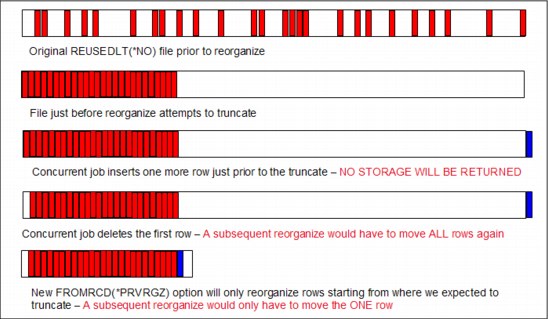
Figure 5-13 Database reorganize worst case example
5.3.26 CPYFRMIMPF performance
Before this enhancement, when you issue the Copy from Import File (CPYFRMIMPF) command from an IFS file into a database file, the data in the IFS file for each character-string column of the database file was converted separately. Typically, all character-string columns of a table or physical file have the same CCSID. With this enhancement, the data for all the character-string columns of such a table or physical file can be converted in one operation rather than separately. This action can drastically reduce the processor that is used and the elapsed time for the Copy from Import File (CPYFRMIMPF). The more columns the table or physical file has, the larger the performance benefit.
5.3.27 QJOSJRNE API option to force journal entries without sending an entry
This enhancement provides a new option to force the journal receiver without sending an entry. If key 4 (FORCE) has a value of 2, the journal receiver is forced without sending an entry. If option 2 is specified, then key 4 must be the only key specified and the length of the entry data must be zero.
A force journal entry is an entry where the journal receiver is forced to auxiliary storage after the user entry is written to it. Possible values are:
0 The journal receiver is not forced to the auxiliary storage. This value is the default value if the key is not specified.
1 The journal receiver is forced to the auxiliary storage.
2 The journal receiver is forced to the auxiliary storage, but no journal entry is sent. When this value is specified, key 4 can be the only key specified and zero must be specified for the length of entry data. Specifying any other keys or a value other than zero for the length of entry data results in an error.
5.3.28 QDBRTVSN API performance
Before this enhancement, finding the short name for a given long name of a table or view was processed by enqueuing a request to the database cross-reference job. That job looks up the short name in the cross-reference.
The QDBRTVSN() API now finds the short name in most cases without enqueuing a request to the database cross-reference.
5.3.29 Control blocking for a file using QSYS2.OVERRIDE_TABLE()
Controlling the blocking size is important for data intensive, performance critical applications.
The Override with Data Base File (OVRDBF) command can be used to tune sequential read-only and write-only applications. A specific byte count can be supplied, or the *BUF32KB, *BUF64KB, *BUF128KB, *BUF256KB special values can be specified.
The OVERRIDE_TABLE() procedure is an easy approach for SQL applications to control blocking programmatically.
Example 5-26 shows overriding a table to use 256K blocking for sequential processing.
Example 5-26 Overriding a table to use 256K blocking for sequential processing
CALL QSYS2.OVERRIDE_TABLE('CORPDATA', 'EMP', '*BUF256KB'),
Example 5-27 shows discarding the override.
Example 5-27 Discarding the override
CALL QSYS2.OVERRIDE_TABLE('CORPDATA', 'EMP', 0);
5.3.30 Improving JDBC performance with JTOpen
This JTOpen enhancement improves JDBC performance by allowing blocked fetches to be used with asensitive cursors for all cursor ResultSet types.
In JDBC, a cursor ResultSet type can be declared as TYPE_FORWARD_ONLY, TYPE_SCROLL_INSENSITIVE, or TYPE_SCROLL_SENSITIVE.
Before the JTOpen 7.9 version of the Toolbox JDBC driver, the DB2 engine only fetched rows in block for the TYPE_FORWARD_ONLY and TYPE_SCROLL_INSENSITIVE types when asensitive was specified for the cursor sensitivity connection property.
This enhancement in JTOpen 7.9 allows the Toolbox JDBC driver to use block fetches with the TYPE_SCROLL_SENSITIVE ResultSet type.
The following is a comparison of the different JDBC cursor ResultSet type settings:
•TYPE_FORWARD_ONLY: Result set can be read only in the forward direction.
•TYPE_SCROLL_INSENSITIVE: Defines the result set as scrollable that allows data to be read from the cursor in any order. The insensitive result set type indicates that recent changes to the rows in the underlying tables should not be visible as the query is executed. The DB2 engine often ensures the insensitive nature of the result set by making a copy of the data before it is provided to the JDBC client. Making a copy of the data can affect performance.
•TYPE_SCROLL_SENSITIVE: Defines the result set as scrollable that allows data to be read from the cursor in any order. The sensitive result type indicates that recent changes to the rows in the underlying table are visible as the query is executed.
The cursor sensitivity setting of asensitive allows DB2 to choose the best performing method when implementing the specified cursor definition. The resulting cursor implementation is either sensitive or insensitive.
In the JTOpen 7.9 version of the toolbox JDBC driver, rows for asensitive cursors are fetched in blocks regardless of the value that is specified for the cursor ResultSet type. This enhancement ensures that when the cursor sensitivity setting of asensitive is specified, both the DB2 engine and the toolbox JDBC driver can use implementations that deliver the best performance.
Example 5-28 shows an example of the JTOpen asensitive cursor.
|
JTOpen Lite: JTOpen Lite does not support scrollable cursors, so this enhancement does not apply to JTOpen Lite applications.
|
Example 5-28 JTOpen asensitive cursor
Connection connection =
DriverManager.getConnection("jdbc:as400://hostname;cursor sensitivity=asensitive", userId, password);
Statement s =
connection.createStatement(ResultSet.TYPE_SCROLL_SENSITIVE,
ResultSet.CONCUR_READ_ONLY);
ResultSet rs = s.executeQuery("SELECT col1, col2 FROM mytable");
Using this JTOpen enhancement, IBM i Navigator and Navigator for i performance was improved when working with large data sets within the On Demand Performance Center:
•Data is blocked when client communicates with IBM i host.
•Ordering of data occurs on the host instead of on the client.
•Object lists within a schema are also improved.
5.3.31 Adding total DB opens job level instrumentation to Collection Services
Collection Services can be used to observe the total number of SQL full opens, SQL pseudo-opens, and the total number of databases full opens (SQL and native I/O). The database has instrumented the number of full opens that occur within a job. This metric is reported by Collection Services in the QAPMJOBOS file.
The new and existing fields contain the total number of times the specific operation occurred within the job during the Collection Services time interval.
Here are the new fields:
Field Name - JBNUS The number of native database (non-SQL) files and SQL cursors that are fully opened. Subtracting the value within field JBLBO from JBNUS yields the number of non-SQL full opens.
Here are the existing fields (for SQL Cursors):
Field Name - JBLBO The cumulative number of SQL cursors that are fully opened.
Field Name - JBLBS The cumulative number of SQL cursors that are pseudo-opened. Pseudo-opens are also known as reused SQL cursors.
5.3.32 SYSTOOLS.REMOVE_INDEXES procedure
You can automate changes to the index strategy by using DB2 for i supplied examples within SYSTOOLS. You can use the DB2 for i procedures directly and pass hardcoded criteria or use the SYSTOOLS source as a fast-start to building your own procedures to manage indexes.
Creating indexes using ACT_ON_INDEX_ADVICE is demonstrated in Example 5-29, which creates permanent SQL indexes from instances of index advice where an MTI was used more than 1000 times.
Example 5-29 Example of index creation
CALL SYSTOOLS.ACT_ON_INDEX_ADVICE(‘PRODLIB’,NULL,NULL,1000,NULL)
The call in Example 5-30 finds indexes that are created by ACT_ON_INDEX_ADVICE that are at least 7 days old. For any index that was used less than 500 times by the Query engine, drop the index.
Example 5-30 Example of index removal
CALL SYSTOOLS.REMOVE_INDEXES(‘PRODLIB’, 500, ' 7 days ')
5.3.33 Improved SQE statistics for INSERT, UPDATE, and DELETE statements
The SQL Query Engine statistics processing now includes a proactive response to data changes as they happen to a database file, rather than just when the file is queried by SQE. The query engine checks for stale statistics during file inserts, updates, or deletes, including INSERT, UPDATE, or DELETE SQL statements.
When stale statistics are detected, a background statistics refresh is initiated, and statistics are refreshed before subsequent query processing, avoiding performance degradation that might occur because of stale statistics being used during query optimization.
This improvement is most beneficial in batched data change environments, such as a data warehouse, where many data change operations occur at one time and are followed by the execution of performance critical SQL queries.
5.3.34 QSYS2.Reset_Table_Index_Statistics procedure
This procedure zeros the QUERY_USE_COUNT and QUERY_STATISTICS_COUNT usage statistics for indexes over the specified tables.
These counts are also zeroed by the CHGOBJD command, but the command requires an exclusive lock. This procedure does not require an exclusive lock.
LAST_QUERY_USE, LAST_STATISTICS_USE, LAST_USE_DATE, and NUMBER_DAYS_USED are not affected.
The same wildcard characters (_ and %) allowed in the SQL LIKE predicate are supported.
The procedure writes information that is related to any index processed into an SQL global temporary table.
The following query displays the results of the last call to the procedure:
select * from session.SQL_index_reset;
In Example 5-31, calls are made to zero the statistics for all indexes over a table, followed by a call to zero the statistics for all indexes over a table, starting with CAT and using the wildcard %.
Example 5-31 Using Reset_Table_Index_Statistics
The following call will zero the statistics for all indexes over table STATST.CATHDANAA
call QSYS2.Reset_Table_Index_Statistics ('STATST', 'CATHDANAA')
The following call will zero the statistics for all indexes over any table in schema STATST whose name starts with the letters CAT
call QSYS2.Reset_Table_Index_Statistics ('STATST', 'CAT%')
5.3.35 Performance enhancements for large number of row locks
Performance of row locking is enhanced for cases where a transaction or job acquires many locks.
Before this enhancement, the more row locks that were acquired on a table, the slower each additional row lock was acquired.
A marked improvement is seen in performance, as shown in Figure 5-14.

Figure 5-14 Row lock performance enhancement
5.3.36 Improved DSPJOB and CHKRCDLCK results for many row locks
The Check Record Locks (CHKRCDLCK) command returns the number of record locks in the current job. The performance of CHKRCDLCK is improved when many record locks are held by the job.
The Display Job (DSPJOB) command allows you to return the locks that are held by a job. If more records are held than can be displayed, a CPF9898 message is sent that indicates the number of record locks that are held by the job.
When a job holds more than 100,000 record locks, both of these commands run for a long time before they fail. The enhancement quickly recognizes the existence of a great number of record locks and returns the record lock count.
5.3.37 Chart-based graphical interface SQL performance monitors
This enhancement allows you to view several high-level charts for specific SQL performance monitors, SQL plan cache snapshots, or SQL plan cache event monitors.
Starting the Investigate Performance Data action from System i Navigator or IBM Navigator for i displays the new graphical interface for SQL Performance monitors, as shown in Figure 5-15.

Figure 5-15 SQL performance monitors
5.3.38 Enhanced analyze program summary detail
The IBM i Navigator SQL Performance Monitor (also known as Database Monitor) Analyze facility is enhanced to produce summarized I/O detail by Program Name.
To see a break-down of I/O activity by program name, analyze a SQL performance monitor and select the program summary. Then, look for the following new columns:
•Synchronous Database Reads
•Synchronous Database Writes
•Asynchronous Database Reads
•Asynchronous Database Writes
See Figure 5-16.

Figure 5-16 Launching the program summary
5.3.39 Performance Data Investigator
This section covers enhancements to the Performance Data Investigator.
New Database perspective
The New Database perspective is a robust graphical interface that is enabled by Collection Services Support. The new breakdown makes it easier to view changes, as shown in Figure 5-17.

Figure 5-17 New Database Perspective
SQL Overview
The SQL Overview contains 11 views. Figure 5-18 illustrates the Query Time Summary view, which is one of the 11 views.

Figure 5-18 SQL Overview: Query Time Summary view
SQL Attribute Mix
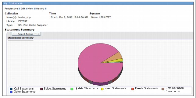
Figure 5-19 SQL Attribute Mix: Statement summary view
5.3.40 Index Advisor: Show Statements - Improved query identification
The Show Statements view of the Index Advisor now uses precise filtering of the SQL Plan Cache. Before this enhancement, the Show Statements view showed all the queries that referenced the target table where the index advice was generated.
Show Statements finds queries based on how it is started:
•If you start it from Index Advice (exact match), it shows Keys Advised, Leading Order Independent Keys, NLSS Table and Schema, Index Type, and Page Size.
•If you use direct Show Statements (table match), you can select the index advice and table name filters.
An advanced form of the SQL Plan cache statements filter is populated by IBM i Navigator, as shown in Figure 5-20.
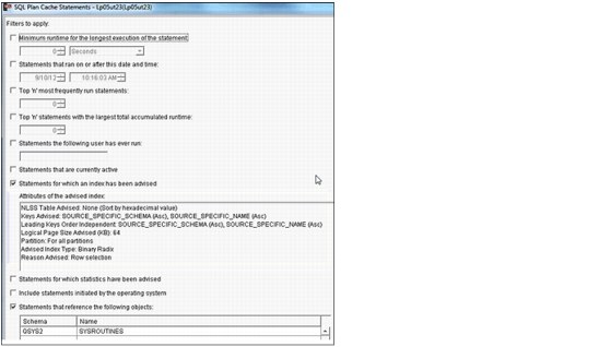
Figure 5-20 An advanced form of the SQL Plan Cache Statements filter populated by IBM i Navigator
These attributes cannot be directly modified by the user.
5.3.41 Performance improvements for temporary tables
The DECLARE GLOBAL TEMPORARY TABLE WITH REPLACE SQL statement might complete much faster when the same table is created again in the same job. In most cases, if the SQL statement text is identical to the previous table, the table is cleared instead of dropped and re-created.
Also, the SQL Plan Cache is improved to recognize the cases where the temporary table is reused with an identical table format. The plan cache plan and statistics management is improved to retain and reuse plans for temporary tables.
Although the overall performance characteristics of temporary tables continue to improve, it is not the best performing choice when you deal with large amounts of data in a performance critical environment.
5.4 New functionality for DB2 developers
This section covers the new functionality for DB2 for i developers.
5.4.1 QSYS2.SYSCOLUMNS2
QSYS2.SYSCOLUMNS2 is a view that is based on a table function that returns more information that is not available in SYSCOLUMNS (such as the allocated length of a varying length column). Because it is based on a table function, it typically returns results faster if a specific table is specified when querying it.
For more information about the view, go to:
http://publib.boulder.ibm.com/infocenter/iseries/v7r1m0/index.jsp?topic=%2Fdb2%2Frbafzcatsyscol2.htm
5.4.2 QSYS2.SYSPARTITIONDISK and QSYS2.SYSPARTITIONINDEXDISK
These two catalog views return allocation information for tables and indexes. The views can be useful in determining how much storage for a partition of index is allocated on an SSD.
For more information, see the SQL Reference at:
Example 5-32 shows the return allocation information for DB2 tables and physical files
in MJATST.
in MJATST.
Example 5-32 Return allocation information for DB2 tables and physical files in MJATST
SELECT MAX(table_schema) AS table_schema, MAX(table_name) AS table_name,
MAX(table_partition) AS table_partition,
SUM(CASE WHEN unit_type = 1 THEN unit_space_used ELSE null END) AS ssd_space,
SUM(CASE WHEN unit_type = 0 THEN unit_space_used ELSE null END) AS non_ssd_space
FROM qsys2.syspartitiondisk a
WHERE system_table_schema = 'MJATST'
GROUP BY a.table_schema, a.table_name, table_partition
ORDER BY 1,2,3;
Figure 5-21 shows the results of Example 5-32 on page 215.
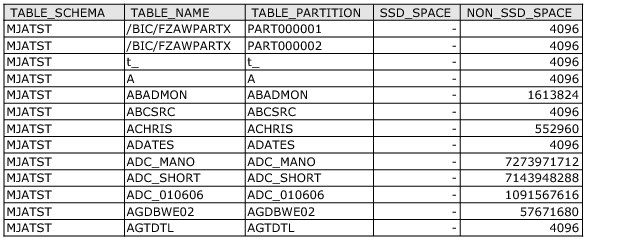
Figure 5-21 Results of Example 5-32 on page 215
Example 5-33 shows the return allocation information for DB2 indexes (keyed files, constraint, and SQL indexes) in MJATST.
Example 5-33 Return allocation information for DB2 indexes (keyed files, constraint, and SQL indexes) in MJATST
SELECT index_schema, index_name, index_member, index_type,
SUM(CASE unit_type WHEN 1 THEN unit_space_used ELSE 0 END)/COUNT(*) AS ssd_space,
SUM(CASE unit_type WHEN 0 THEN unit_space_used ELSE 0 END)/COUNT(*) AS nonssd_space
FROM qsys2.syspartitionindexdisk b
WHERE system_table_schema = 'MJATST'
GROUP BY index_schema, index_name, index_member, index_type;
SUM(CASE unit_type WHEN 1 THEN unit_space_used ELSE 0 END)/COUNT(*) AS ssd_space,
SUM(CASE unit_type WHEN 0 THEN unit_space_used ELSE 0 END)/COUNT(*) AS nonssd_space
FROM qsys2.syspartitionindexdisk b
WHERE system_table_schema = 'MJATST'
GROUP BY index_schema, index_name, index_member, index_type;
Figure 5-22 shows the results of Example 5-33.

Figure 5-22 Results of Example 5-33
5.4.3 QSYS2.OBJECT_STATISTICS user defined table function
The OBJECT_STATISTICS table function returns information about objects in a library. The schema is QSYS2. Following is the format of the OBJECT_STATISTICS table function:
OBJECT_STATISTICS (library-name, object-type-list )
Where:
•library-name is a character or graphic string expression that identifies the name of a library. It can be either a long or short library name.
•object-type-list is a character or graphic string expression that contains one or more system object types separated by either a blank or a comma. The object types can include or exclude the leading * character. For example, either FILE or *FILE can be specified.
Following are some examples of using OBJECT_STATISTICS table function:
•Find all journals in library MJATST:
SELECT * FROM TABLE (QSYS2.OBJECT_STATISTICS('MJATST ','JRN') ) AS X
or
SELECT * FROM TABLE (QSYS2.OBJECT_STATISTICS('MJATST ','*JRN') ) AS X
•Find all journals and journal receivers in library MJATST:
SELECT * FROM TABLE (QSYS2.OBJECT_STATISTICS('MJATST ','JRN JRNRCV') ) AS X
or
SELECT * FROM TABLE (QSYS2.OBJECT_STATISTICS('MJATST ','*JRN *JRNRCV') ) AS X
The result of the function is a table that contains a row for each object with the format shown in Table 5-4. All the columns are nullable.
Table 5-4 OBJECT_STATISTICS table function
|
Column Name
|
Data Type
|
Description
|
|
OBJNAME
|
VARCHAR(10)
|
System name of the object.
|
|
OBJTYPE
|
VARCHAR(8)
|
System type of the object.
|
|
OBJOWNER
|
VARCHAR(10)
|
User profile that owns the object.
|
|
OBJDEFINER
|
VARCHAR(10)
|
User profile that created the object.
|
|
OBJCREATED
|
TIMESTAMP
|
Timestamp of when the object was created.
|
|
OBJSIZE
|
DECIMAL(15,0)
|
Size of the object, in bytes.
|
|
OBJTEXT
|
VARCHAR(50)
|
Description of the object.
|
|
OBJLONGNAME
|
VARCHAR(128)
|
Long description of the object.
|
|
LAST_USED_TIMESTAMP
|
TIMESTAMP
|
Date the object was used last.
|
|
DAYS_USED_COUNT
|
INTEGER
|
Number of days an object has been used on the system.
|
|
LAST_RESET_TIMESTAMP
|
TIMESTAMP
|
Date when the days used count was last reset to zero.
|
|
IASP_NUMBER
|
SMALLINT
|
Auxiliary storage pool (ASP) where storage is allocated for the object.
|
|
OBJATTRIBUTE
|
VARCHAR(5)
|
Attribute for this objects type, if any.
|
5.4.4 EARLIEST_POSSIBLE_RELEASE
DB2 for i now provides a way to see the earliest IBM i release that can be used for any SQL statement or program. The SQL statement level detail is available through Database Monitor. The program level detail is available through the QSYS2.SYSPROGRAMSTAT and QSYS2.SYSPACKAGESTAT catalogs. In both cases, you must capture the DBMON or rebuild the program after you apply the latest DB Group PTFs.
Database Monitor and the QSYS2.SYSPROGRAMSTAT and QSYS2.SYSPACKAGESTAT catalogs can be used to evaluate SQL application deployment possibilities per operating system releases. The QQC82 column contains the earliest IBM i OS release level where this SQL statement is supported. This information can be used to assess whether applications can be deployed on earlier IBM i releases or whether they are using SQL functions unique to IBM i 6.1 or 7.1.
This field applies only if the SQL statement is dynamic (QQC12= 'D').
Possible values for QQC82 are:
' The statement release level is not determined.
'ANY' The statement is valid on any supported IBM i OS release,
'V6R1M0' The statement is valid on IBM i 6.1 or later.
'V7R1M0' The statement is valid on IBM i 7.1 or later.
The QSYS2.SYSPROGRAMSTAT and QSYS2.SYSPACKAGESTAT column name is EARLIEST_POSSIBLE_RELEASE. The System column name is MINRLS.
5.4.5 SIGNAL support for native triggers
INSERT, UPDATE, and DELETE SQL statements were changed to recognize when system triggers use the SIGNAL SQL statement to communicate failure details to the application.
If the system trigger runs the SIGNAL statement and sends an escape message to its caller, the SQL INSERT, UPDATE, or DELETE statement fails with MSGSQL0438 (SQLCODE=-438) instead of MSGSQL0443.
The SQLSTATE, MSG, and other values within the SQL diagnostics area or SQLCA contain the values that are passed into the SIGNAL statement.
For more information, go to:
The website contains recommendations for native trigger programs. Here is an example:
“Signal an exception if an error occurs or is detected in the trigger program. If an error message is not signaled from the trigger program, the database assumes that the trigger ran successfully. This might cause the user data to end up in an inconsistent state.”
The SIGNAL SQL statement provides the SQL linkage between the native trigger and the application that causes the trigger to be fired by using SQL.
The SIGNAL SQL statement does not signal an exception, so be sure to use the QMHSNDPM() API to send an escape message after you run the SIGNAL statement, as shown in Example 5-34.
Example 5-34 JDBC failure
*** SQLException caught ***
Statement was insert into mylib.mytable values(1)
SQLState: IWF99
Message: [SQL0438] DOCUMENT NOT FOUND
Vendor: -438
java.sql.SQLException: [SQL0438] DOCUMENT NOT FOUND
at com.ibm.as400.access.JDError.throwSQLException(JDError.java:650)
etc.....
5.4.6 Hierarchical queries through the CONNECT BY clause
DB2 for i has had recursive query support since V5R4. Another recursive query technique called hierarchical query was added. This technique is a more concise method of representing a recursive query.
For more information, see the IBM i 7.1 Knowledge Center at the following websites:
Example 5-35 shows a hierarchal query example.
Example 5-35 Hierarchical query example
CALL QSYS.CREATE_SQL_SAMPLE('MYDB'),
SET CURRENT SCHEMA MYDB;
SET CURRENT PATH MYDB;
SET CURRENT SCHEMA MYDB;
SET CURRENT PATH MYDB;
SELECT LEVEL,
CAST(SPACE((LEVEL - 1) * 4) || '/' || DEPTNAME AS VARCHAR(40)) AS DEPTNAME
FROM DEPARTMENT
START WITH DEPTNO = 'A00'
CONNECT BY NOCYCLE PRIOR DEPTNO = ADMRDEPT
Figure 5-23 shows the result of Example 5-35 on page 219.
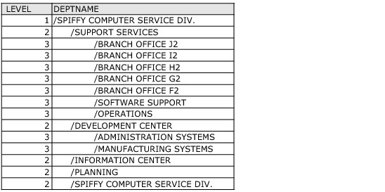
Figure 5-23 Result of hierarchical query
5.4.7 Parameter marker support (LAND, LOR, XOR, and TRANSLATE)
Before IBM i 7.1, there were many restrictions on where a parameter marker was allowed in an SQL statement. Many of these restrictions were removed in IBM i 7.1.
The LAND, LOR, XOR, and TRANSLATE scalar functions were enhanced by removing similar restrictions.
Example 5-36 shows the possible usage of parameter markers.
Example 5-36 Possible usage of parameter markers
PREPARE s1 FROM ‘SELECT TRANSLATE(c1,?,?,?) FROM t1’
PREPARE s1 FROM ‘SELECT LAND(c2,?,?,?), LOR(c2,?,?,?), XOR(c2,?,?,?) FROM t1’ 
5.4.8 Supporting PROGRAM NAME on CREATE TRIGGER
It is now possible to specify a short name for the created trigger program. When this specification is not supplied, the database determines the system name, which might lead to differences in the system name for the trigger program across different systems.
Example 5-37 shows the usage of PROGRAM NAME in the CREATE TRIGGER definition. If a program name is not specified, then the system generates one, such as TR1_U00001 or TR1_U00002.
Example 5-37 Usage of PROGRAM NAME in the CREATE TRIGGER definition
CREATE TRIGGER TR1_UPDATE_TRACKER
AFTER UPDATE OF c1 ON TR1
REFERENCING OLD AS o NEW AS n
FOR EACH ROW MODE DB2ROW
PROGRAM NAME TR1_UPTRIG
BEGIN ATOMIC
INSERT INTO tr2 VALUES(default, o.c1, n.c1);
END
5.4.9 Debug step supported for SQL procedures, functions, and triggers
SQL procedures, functions, and triggers created with SET OPTION DBGVIEW = *SOURCE can be debugged using the following:
•Using the Start Debug (STRDBG) command
•Using IBM i Navigator System Debugger
When an SQL procedure, function, or trigger is built for debug, two debug views can be used:
•SQL Object Processor Root View (default)
•Underlying ILE C listing view
Before this enhancement, when the Step function (F10=Step when using STRDBG or F11=Step Over when using System Debugger) was used within either of the IBM i debuggers at the SQL view debug level, the Step action applied to the underlying ILE C listing view. It normally takes many steps at the SQL debug view level to get to the next statement, making the SQL debug view difficult to use.
After this enhancement is installed, the Step action applies at the SQL Statement view level. This enhancement makes it much easier to debug SQL procedures, functions, and triggers.
5.4.10 TINYINT in CLI
This SQL Call Level Interface (CLI) enhancement allows applications using CLI APIs for binding parameters and output fields for result sets to accept a new bind type named SQL_C_UTINYINT, Unsigned TINYINT. This bind type represents a 1-byte unsigned integer value with values 0 - 255.
For more information, see the IBM i 7.1 SQL CLI documentation at:
5.4.11 CHGPFM and CHGLFM UNIT support
Change Physical File Member (CHGPFM) and Change Logical File Member (CHGLFM) commands can now be used to move an individual member to or from an SSD by changing the media preference. One of the main benefits of using these commands is that they do not require a LENR lock. However, they conflict with another job that has an *SHRNUP, *EXCLRD, or *EXCL lock on the data. The syntax of these commands is as follows:
•CHGPFM t1 UNIT(*SSD)
•CHGLFM v1 UNIT(*SSD)
If the user is using logical replication, you need the PTFs on the target and the source systems.
5.4.12 Live movement of DB2 tables and indexes to SSD
The media preference on a DB2 for i tables, views, and indexes can be changed without requiring an exclusive, no read lock on the file. The change can be made when shared read locks (*SHRRD) exist on the file.
After *SSD has been specified as the preferred storage media, the file data is asynchronously moved to the SSD.
This enhancement applies to the following SQL and IBM i command interfaces:
•ALTER TABLE STORE123.EMPLOYEE ALTER UNIT SSD
•CHGPF FILE(STORE123/EMPLOYEE) UNIT(*SSD)
•CHGLF FILE(STORE123/XEMP2) UNIT(*SSD)
For more information about SSDs, see the following references:
•How to boost application performance using Solid State Disk drives
•DB2 for i Hitting the Mark - Again
5.4.13 SYSTOOLS procedures
SYSTOOLS is a set of DB2 for i supplied examples and tools. SYSTOOLS is the name of a database supplied schema (library). SYSTOOLS differs from other DB2 for i supplied schemas (QSYS, QSYS2, SYSIBM, and SYSIBMADM) in that it is not part of the default system path. As general-purpose useful tools or examples that are built by IBM, they are considered for inclusion within SYSTOOLS. SYSTOOLS provides a wider audience with the opportunity to extract value from the tools.
It is the intention of IBM to add content dynamically to SYSTOOLS, either on base releases or through PTFs for field releases. A preferred practice for customers who are interested in such tools is to periodically review the contents of SYSTOOLS.
For more information, see the IBM Knowledge Center at:
5.4.14 HTTP functions in SYSTOOLS
HTTP is the preferred way for communicating in resource-oriented architecture (ROA) and service-oriented architecture (SOA) environments. You can use these RESTful services to integrate information sources that can be addressed using a URL and accessed using HTTP.
The DB2 for i HTTP functions are defined in the SYSTOOLS schema (home of DB2 for i supplied tools and examples) and are not covered by IBM Software Maintenance and Support. These functions are ready for use and provide a fast start to building your own applications.
These DB2 for i HTTP functions require Java 1.6 (5761-JV1).
The functions are also visible with IBM Navigator for i.
Following are the HTTP UDF names:
•httpGetBlob
•httpGetClob
•httpPutBlob
•httpPutClob
•httpPostBlob
•httpPostClob
•httpDeleteBlob
•httpDeleteClob
•httpBlob
•httpClob
•httpHead
Example 5-38 shows an example of the using the DB2 for i HTTP functions to consume information from a blog.
The following steps show you how to use the DB2 for i HTTP functions to consume information from URL. In this example, information from the DB2 for i blog is consumed.
1. Build a utility function to manage the content time stamp:
CREATE OR REPLACE FUNCTION QGPL.RFC339_DATE_FORMAT(in_time TIMESTAMP)
RETURNS VARCHAR(26)
LANGUAGE SQL
RETURN CAST(DATE(in_time) AS CHAR(10)) || 'T' || CHAR(TIME(in_time), JIS)
2. Use XML features on DB2 for i 7.1 to query the blog content and return the blog posts for the last 6 months. (order the rows by reader responses). See Example 5-38.
Example 5-38 Using DB2 for i HTTP functions to consume information from a blog
-- Blog Posts for the last 6 months, order by reader responses
SELECT published, updated, author, title, responses, url, author_bio, html_content, url_atom
FROM
XMLTABLE(
XMLNAMESPACES(DEFAULT 'http://www.w3.org/2005/Atom',
'http://purl.org/syndication/thread/1.0' AS "thr"),
'feed/entry'
PASSING XMLPARSE(DOCUMENT
SYSTOOLS.HTTPGETBLOB(
-- URL --
'http://db2fori.blogspot.com/feeds/posts/default?published-min=' ||
SYSTOOLS.URLENCODE(QGPL.RFC339_DATE_FORMAT(CURRENT_TIMESTAMP - 6 MONTHS), 'UTF-8') ||
'&published-max=' || SYSTOOLS.URLENCODE(QGPL.RFC339_DATE_FORMAT(CURRENT_TIMESTAMP + 1 DAYS) , 'UTF-8') ,
-- header --
'<httpHeader> <header name="Accept" value="application/atom+xml"/> </httpHeader>'
) )
COLUMNS
published TIMESTAMP PATH 'published',
updated TIMESTAMP PATH 'updated',
author VARCHAR(15) CCSID 1208 PATH 'author/name',
title VARCHAR(100) CCSID 1208 PATH 'link[@rel="alternate" and @type="text/html"]/@title',
responses INTEGER PATH 'thr:total',
author_bio VARCHAR(4096) CCSID 1208 PATH 'author/uri',
url VARCHAR(4096) CCSID 1208 PATH 'link[@rel="alternate" and @type="text/html"]/@href',
url_atom VARCHAR(4096) CCSID 1208 PATH 'link[@rel="self" and @type="application/atom+xml"]/@href',
html_content CLOB CCSID 1208 PATH 'content[@type="html"]'
) RS
ORDER BY RESPONSES DESC
3. Examine the output as shown in Figure 5-24.
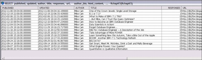
Figure 5-24 Results from consuming information from a blog
For more information about DB2 for i HTTP functions, see the following websites:
•Accessing web services: Using IBM DB2 for i HTTP UDFs and UDTFs:
•Accessing HTTP and RESTful services from DB2: Introducing the REST user-defined functions for DB2:
5.4.15 QSYS2.TCPIP_INFO view
The TCPIP_INFO view contains TCP/IP information for the current host connection.
|
Note: This support does not cover when TELNET is used to form the connection.
|
Table 5-5 describes the columns in the view.
Table 5-5 TCPIP_INFO view
|
Column Name
|
System Column Name
|
Data Type
|
Description
|
|
COLLECTED_TIME
|
COLLE00001
|
TIMESTAMP
Nullable
|
Timestamp indicating when this row of information was collected.
|
|
LOCAL_HOST_NAME
|
LOCAL00001
|
VARCHAR(255)
Nullable
|
TCP/IP host name of the local system.
|
|
CLIENT_IP_ADDRESS_TYPE
|
CLIEN00001
|
VARCHAR(10)
Nullable
|
TCP/IP address version of client.
|
|
CLIENT_IP_ADDRESS
|
CLIEN00002
|
VARCHAR(45)
Nullable
|
TCP/IP address of the client.
|
|
CLIENT_PORT_NUMBER
|
CLIEN00003
|
INTEGER
Nullable
|
TCP/IP port of the client.
|
|
SERVER_IP_ADDRESS_TYPE
|
SERVE00001
|
VARCHAR(10)
Nullable
|
TCP/IP address version of the server.
|
|
SERVER_IP_ADDRESS
|
SERVE00002
|
VARCHAR(45)
Nullable
|
TCP/IP address of the server.
|
|
SERVER_PORT_NUMBER
|
SERVE00003
|
INTEGER
Nullable
|
TCP/IP port number of the server.
|
|
HOST_VERSION
|
HOST_00001
|
VARCHAR(10)
Nullable
|
Operating system version.
|
The following statement shows usage of QSYS2.TCPIP_INFO:
SELECT * from QSYS2.TCPIP_INFO
Figure 5-25 shows the results of using QSYS2.TCPIP_INFO.
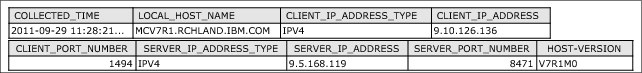
Figure 5-25 Results of QSYS2.TCPIP_INFO
5.4.16 Administrative catalog, SYSIBMADM.ENV_SYS_INFO
The ENV_SYS_INFO view contains information about the current server.
Table 5-6 describes the columns in the ENV_SYS_INFO view. The schema is SYSIBMADM.
Table 5-6 ENV_SYS_INFO view
|
Column Name
|
System Column Name
|
Data Type
|
Description
|
|
OS_NAME
|
OS_NAME
|
VARCHAR(256)
Nullable
|
Operating system name
|
|
OS_VERSION
|
OS_VERSION
|
VARCHAR(256)
Nullable
|
Operating system version
|
|
OS_RELEASE
|
OS_RELEASE
|
VARCHAR(256)
Nullable
|
Operating system release
|
|
HOST_NAME
|
HOST_NAME
|
VARCHAR(256)
Nullable
|
Name of the system
|
|
TOTAL_CPUS
|
TOTAL_CPUS
|
INTEGER
Nullable
|
Total number of physical CPUs on the system
|
|
CONFIGURED_CPUS
|
CONFIGCPUS
|
INTEGER
Nullable
|
Total number of configured CPUs on the system
|
|
TOTAL_MEMORY
|
TOTAL_MEM
|
INTEGER
Nullable
|
Total amount of memory on the system, in megabytes
|
Figure 5-26 shows an example of the output from ENV_SYS_INFO.

Figure 5-26 ENV_SYS_INFO output
5.4.17 QSYS2.PTF_INFO view
The PTF_INFO view in QSYS2 contains information about PTFs for the server. The data that are returned by this view corresponds to the data returned by the List Program Temporary Fixes (QpzListPTF) API.
For more information about the QpzListPTF) API, see the List Program Temporary Fixes (QpzListPTF) API topic in the IBM i 7.1 Knowledge Center:
Table 5-7 describes the columns in the PTF_INFO view. The schema is QSYS2.
Table 5-7 PTF_INFO view
|
Column name
|
System Column Name
|
Data Type
|
Description
|
|
PTF_PRODUCT_ID
|
LICPGM
|
VARCHAR(7)
Nullable
|
Product identifier.
|
|
PTF_PRODUCT_OPTION
|
PRODOPT
|
VARCHAR(6)
Nullable
|
Product option.
|
|
PTF_PRODUCT_RELEASE_LEVEL
|
PRODRLS
|
VARCHAR(6)
Nullable
|
Product release level.
|
|
PTF_PRODUCT_DESCRIPTION
|
PRODDESC
|
VARCHAR(132)
Nullable
|
Product description.
|
|
PTF_IDENTIFIER
|
PTFID
|
VARCHAR(7)
Nullable
|
The identifier of the PTF.
|
|
PTF_RELEASE_LEVEL
|
PTFRLS
|
VARCHAR(6)
Nullable
|
The release level of the PTF.
|
|
PTF_PRODUCT_LOAD
|
PRODLOAD
|
VARCHAR(4)
Nullable
|
The load ID of the product load for the PTF.
|
|
PTF_LOADED_STATUS
|
LOADSTAT
|
VARCHAR(19)
Nullable
|
The current loaded status of the PTF:
•NOT LOADED - The PTF has never been loaded.
•LOADED - The PTF has been loaded.
•APPLIED - The PTF has been applied.
•PERMANENTLY APPLIED - The PTF has been applied permanently.
•PERMANENTLY REMOVED - The PTF has been permanently removed.
•DAMAGED - The PTF is damaged. An error occurred while applying the PTF. The PTF needs to be reloaded and applied again.
•SUPERCEDED - The PTF is superseded. A PTF has a status of superseded when one of the following situations occurs:
– Another PTF with a more recent correction for the problem has been loaded on the system. The PTF ID that has been loaded can be found in the PTF_SUPERCEDED_BY_PTF column.
– The PTF save file for another PTF with a more recent correction for the problem has been logged in to *SERVICE on the system.
|
|
PTF_SAVE_FILE
|
SAVF
|
VARCHAR(3)
Nullable
|
Indicates whether a save file exists for the PTF:
•NO - The PTF has no save file.
•YES - The PTF has a save file.
|
|
PTF_COVER_LETTER
|
COVER
|
VARCHAR(3)
Nullable
|
Indicates whether a cover letter exists for the PTF:
•NO - The PTF has no cover letter.
•YES - The PTF has a cover letter.
|
|
PTF_ON_ORDER
|
ONORD
|
VARCHAR(3)
Nullable
|
Indicates whether the PTF has been ordered.:
•NO - The PTF has not been ordered or has already been received.
•YES - The PTF has been ordered.
|
|
PTF_IPL_ACTION
|
PLACT
|
VARCHAR(19)
Nullable
|
The action to be taken on this PTF during the next unattended IPL:
•NONE - No action occurs at the next IPL.
•TEMPORARILY APPLIED - The PTF is temporarily applied at the next IPL.
•TEMPORARILY REMOVED - The PTF is temporarily removed at the next IPL.
•PERMANENTLY APPLIED - The PTF is permanently applied at the next IPL.
•PERMANENTLY REMOVED - The PTF is permanently removed at the next IPL.
|
|
PTF_ACTION_PENDING
|
ACTPEND
|
VARCHAR(3)
Nullable
|
Indicates whether a required action has yet to be run to make this PTF active:
•NO - No required actions are pending for this PTF.
•YES - A required action needs to occur for this PTF to be active. Check the Activation Instructions section of the cover letter to determine what the action is. If the PTF_ACTION_REQUIRED column is set to IPL and the activation instructions have been performed, then the PTF is active. However, this column is not updated until the next IPL.
|
|
PTF_ACTION_REQUIRED
|
ACTREQ
|
VARCHAR(12)
Nullable
|
Indicates whether an action is required to make this PTF active when it is applied. See the cover letter to determine what action needs to be taken.
•NONE - No activation instructions are needed for this PTF.
•EXIT PROGRAM -, This PTF was included with activation instructions in the cover letter. This value is returned for all PTFs that have an exit program to update the status of the PTF after the activation instructions have been performed.
•IPL - This PTF was included with activation instructions in the cover letter. No exit program exists to verify that the activation instructions were performed.
|
|
PTF_IPL_REQUIRED
|
PLREQ
|
VARCHAR(9)
Nullable
|
Indicates whether an IPL is required to apply this PTF:
•DELAYED - The PTF is delayed. The PTF must be applied during an IPL.
•IMMEDIATE - The PTF is immediate. No IPL is needed to apply the PTF.
•UNKNOWN - The type of the PTF is not known.
|
|
PTF_IS_RELEASED
|
RELEASED
|
VARCHAR(3)
Nullable
|
Indicates whether the PTF save file is available for distribution to another system. This is set to YES only when the system manager for the IBM i licensed program is on the system and the product is supported. The PTF_SAVE_FILE column must have a value of YES before using the value in this column:
•NO - The PTF save file cannot be distributed.
•YES - The PTF save file is released and can be distributed to another system.
|
|
PTF_MINIMUM_LEVEL
|
MINLVL
|
VARCHAR(2)
Nullable
|
The indicator of the lowest level of the product to which this PTF can be applied. The level can be AA to 99. Contains the null value if the product does not have a level.
|
|
PTF_MAXIMUM_LEVEL
|
MAXLVL
|
VARCHAR(2)
Nullable
|
The indicator of the highest level of the product to which this PTF can be applied. The level can be AA to 99. Contains the null value if the product does not have a level.
|
|
PTF_STATUS_TIMESTAMP
|
STATTIME
|
TIMESTAMP
Nullable
|
The date and time that the PTF status was last changed. Contains the null value when the status date and time is not available.
|
|
PTF_SUPERCEDED_BY_PTF
|
SUPERCEDE
|
VARCHAR(7)
Nullable
|
The identifier of the PTF that has replaced this PTF. This field is blank when the PTF is not superseded or when the superseding PTF has not been loaded on the system.
|
|
PTF_CREATION_TIMESTAMP
|
CRTTIME
|
TIMESTAMP
Nullable
|
The date and time that the PTF was created. Contains the null value when the creation date and time cannot be determined.
|
|
PTF_TECHNOLOGY_REFRESH_PTF
|
TRPTF
|
VARCHAR(3)
Nullable
|
Indicates whether this is a technology refresh PTF:
•NO - This is not a technology refresh PTF.
•YES - This is a technology refresh PTF.
|
Example 5-39 and Example 5-40 provide some examples of how the PTF_INFO view can be used. Example 5-39 shows an example when PTFs are impacted by the next IPL.
Example 5-39 Discovering which PTFs are impacted by the next IPL
SELECT PTF_IDENTIFIER, PTF_IPL_ACTION, A.*
FROM QSYS2.PTF_INFO A
WHERE PTF_IPL_ACTION <> 'NONE'
Example 5-40 shows an example when the PTFs are loaded but not applied.
Example 5-40 Discovering which PTFs are loaded but not applied
SELECT PTF_IDENTIFIER, PTF_IPL_REQUIRED, A.*
FROM QSYS2.PTF_INFO A
WHERE PTF_LOADED_STATUS = 'LOADED'
ORDER BY PTF_PRODUCT_ID
5.4.18 QSYS2.GROUP_PTF_INFO view
You can use the QSYS2.GROUP_PTF_INFO view to retrieve IBM i Group PTF information. The data that is returned is similar to output of the Work with PTF Groups (WRKPTFGRP) command.
For example, the Technology Refresh (TR) level on your system can be determined by using the view definition that is shown in Example 5-41.
Example 5-41 Determining the Technology Refresh (TR) level
COLLECTED_TIME FOR COLUMN COLLE00001 TIMESTAMP
PTF_GROUP_NAME FOR COLUMN PTF_G00001 VARCHAR(60) ALLOCATE(60)
PTF_GROUP_DESCRIPTION FOR COLUMN PTF_G00002 VARCHAR(100) ALLOCATE(100)
PTF_GROUP_LEVEL FOR COLUMN PTF_G00003 INTEGER DEFAULT NULL
PTF_GROUP_TARGET_RELEASE FOR COLUMN PTF_G00004 VARCHAR(6) ALLOCATE(6)
PTF_GROUP_STATUS FOR COLUMN PTF_G00005 VARCHAR(20) ALLOCATE(20)
Run the following command:
select * from QSYS2.GROUP_PTF_INFO order by PTF_GROUP_LEVEL DESC;
The result of the command is shown in Figure 5-27.

Figure 5-27 Results from QSYS2.GROUP_PTF_INFO call
The PTF group status messages are:
UNKNOWN The PTF’s group status cannot be resolved because a related PTF group is either not found on the system or is in error.
NOT APPLICABLE All PTFs in the PTF group and related PTF groups are for products that are not installed or supported on this system.
SUPPORTED ONLY There are no PTFs in the PTF group or related PTF groups that are for installed products on this system. There is at least one PTF that is for a product, release, option, and load identifier that is supported on this system.
NOT INSTALLED There is at least one PTF that is for an installed product on this system, and not all of the PTFs or their superseding PTFs are temporarily or permanently applied.
INSTALLED All PTFs for products that are installed on this system are temporarily or permanently applied. If a PTF is superseded, a superseding PTF is either temporarily or permanently applied.
ERROR The PTF group information is in error. Either delete the PTF group or replace the PTF group information that is on the system.
APPLY AT NEXT IPL All PTFs for the installed products on the system are either set to be applied at the next IPL, or are temporarily or permanently applied.
RELATED GROUP The PTF group does not have any PTFs for products that are installed or supported on the system. However, it is identified in another PTF group as a related PTF group. Deleting a PTF group in this status causes the other PTF group to have a status of Unknown.
ON ORDER There is at least one PTF in the group that is on order and has not yet been installed on the system. It can be delivered on either physical or virtual media.
5.4.19 QSYS2.GET_JOB_INFO() user defined table function
The GET_JOB_INFO table function returns one row that contains information about a specific job. Where job-name is a character or graphic string expression that identifies the name of a job. The schema is QSYS2.
>>-GET_JOB_INFO--(--job-name--)--------------------------------><
To start the GET_JOB_INFO table function, the caller must have *JOBCTL user special authority or QIBM_DB_SQLADM or QIBM_DB_SYSMON function usage authority.
The result of the GET_JOB_INFO function is a table that contains a single row with the format shown in Table 5-8. All the columns are nullable.
Table 5-8 GET_JOB_INFO table function
|
Column Name
|
Data Type
|
Description
|
|
V_JOB_STATUS
|
CHAR(10)
|
Status of the job.
|
|
V_ACTIVE_JOB _STATUS
|
CHAR(4)
|
To understand the values that are returned in this field, see this reference and search on “Active job status”: Work Management API Attribute Descriptions. For more information, go to:
|
|
V_RUN _PRIORITY
|
INTEGER
|
The highest run priority allowed for any thread within this job.
|
|
V_SBS_NAME
|
CHAR(10)
|
Name of subsystem where job is running.
|
|
V_CPU_USED
|
BIGINT
|
The amount of CPU time (in milliseconds) that has been used by this job.
|
|
V_TEMP_STORAGE_USED_MB
|
INTEGER
|
The amount of auxiliary storage (in megabytes) that is allocated to this job.
|
|
V_AUX_IO_REQUESTED
|
BIGINT
|
The number of auxiliary I/O requests run by the job across all routing steps. This includes both database and nondatabase paging. This is an unsigned BINARY(8) value.
|
|
V_PAGE_FAULTS
|
BIGINT
|
The number of times an active program referenced an address that is not in main storage during the current routing step of the specified job.
|
|
V_CLIENT_WRKSTNNAME
|
CHAR(255)
|
Value of the SQL CLIENT_WRKSTNNAME special register.
|
|
V_CLIENT_APPLNAME
|
CHAR(255)
|
Value of the SQL CLIENT_APPLNAME special register.
|
|
V_CLIENT_ACCTNG
|
CHAR(255)
|
Value of the SQL CLIENT_ACCTNG special register.
|
|
V_CLIENT_PROGRAMID
|
CHAR(255)
|
Value of the SQL CLIENT_PROGRAMID special register.
|
|
V_CLIENT_USERID
|
CHAR(255)
|
Value of the SQL CLIENT_USERID special register.
|
Figure 5-28 shows the results of the GET_JOB_INFO function,
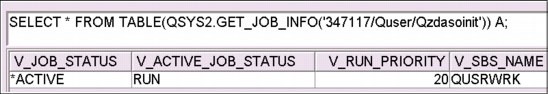
Figure 5-28 GET_JOB_INFO output
5.4.20 Alias interrogation, SYSPROC.BASE_TABLE
The SYSPROC.BASE_TABLE UDTF function provides a cross DB2 method to identify the actual table or view an alias is based on. The following unique DB2 for i information can also be accessed:
•System names
•Member names (for aliases that point to a single member)
•Database name (for aliases that point to a remote object)
For more information about the BASE_TABLE function, see the SQL Reference documentation:
The BASE_TABLE function returns the object names and schema names of the object found for an alias.
Example 5-42 shows an example of determining the base objects for all aliases within the schemas that have “MJATST” somewhere in the schema name
Example 5-42 Using the BASE_TABLE function
SELECT
A.TABLE_SCHEMA AS ALIAS_SCHEMA, A.TABLE_NAME AS ALIAS_NAME, c.*
FROM QSYS2.SYSTABLES A,
LATERAL (
SELECT * FROM TABLE(SYSPROC.BASE_TABLE(A.TABLE_SCHEMA,A.TABLE_NAME)) AS X)
AS C
WHERE A.TABLE_TYPE='A' and upper(table_schema) like '%MJATST%'
Figure 5-29 shows the results of Example 5-42 on page 234.
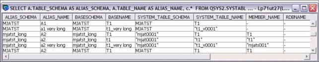
Figure 5-29 Output from alias interrogation
Figure 5-30 shows the BASE_TABLE UDTF parameter definition.
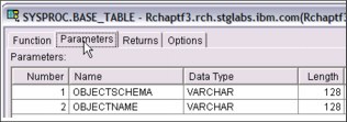
Figure 5-30 BASE_TABLE UDTF parameter definition
Figure 5-31 shows the BASE_TABLE UDTF return table definition.
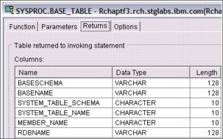
Figure 5-31 BASE_TABLE UDTF return table definition
5.4.21 Number of partition keys added to statistical views
Two of the DB2 for i statistical catalogs have been extended to include the NUMBER_PARTITIONING_KEYS column. This column returns the number of partitioning keys to make it easier for other IBM and third-party products to process the partitioning keys.
The NUMBER_PARTITIONING_KEYS column has been added to the following statistical catalogs:
•QSYS2 and SYSIBM: SYSPARTITIONSTAT
•QSYS2 and SYSIBM: SYSTABLESTAT
For more information, see the SQL Reference at:
Figure 5-32 shows the output for the number of partition keys.

Figure 5-32 Sample output for the number of partition keys
5.4.22 QSYS2.DUMP_SQL_CURSORS procedure
It is now possible to capture the list of open cursors for a job in IBM i. The QSYS2.DUMP_SQL_CURSORS are:
•Job_Name VARCHAR(28),
•Library_Name CHAR(10),
•Table_Name CHAR(10),
•Output_Option integer)
Where:
•Job_Name is a qualified job name or a special value of '*' to indicate the current job.
•Library_Name is an optional library name for the procedure output.
•Table_Name is an optional table name for the procedure output.
Output_Option has these choices:
•Ignore Library_Name and Table_Name inputs and return a result set.
•Ignore Library_Name and Table_Name inputs and place the results in table QTEMP/SQL_CURSORS (no result set).
•Place the results in table in Library_Name and Table_Name (no result set). If the table does not exist, the procedure creates it. If the table does exist, the results are appended to the existing table.
•Place the results in table in Library_Name and Table_Name (no result set). If the table does not exist, do not create the table.
Example 5-43 shows a possible invocation of the QSYS2.DUMP_SQL_CURSORS procedure.
Example 5-43 Possible invocation
-- populate QGPL.SQLCSR1 table with open SQL cursors in this job
call qsys2.DUMP_SQL_CURSORS('*', 'QGPL', 'SQLCSR1', 3);
-- return a result set with open SQL cursors in this job
call qsys2.DUMP_SQL_CURSORS('*', '', '', 1);
-- populate QGPL.SQLCSR1 table with open SQL cursors for a target job
call qsys2.DUMP_SQL_CURSORS('724695/QUSER/QZDASOINIT', '', '', 1);
Table/Result Set format:
SQL_IDENTITY FOR COLUMN SQL_I00001 INTEGER ,
DUMPTIME TIMESTAMP ,
DUMP_BY_USER FOR COLUMN DUMPUSER VARCHAR(18) ,
CURSOR_NAME FOR COLUMN CSRNAME VARCHAR(128) ,
PSEUDO_CLOSED FOR COLUMN PSEUDO VARCHAR(3) ,
STATEMENT_NAME FOR COLUMN STMTNAME VARCHAR(128) ,
OBJECT_NAME FOR COLUMN OBJNAME CHAR(10) ,
OBJECT_LIBRARY FOR COLUMN OBJLIB CHAR(10) ,
OBJECT_TYPE FOR COLUMN OBJTYPE CHAR(10) ,
JOBNAME CHAR(28)
5.4.23 QIBM_SQL_NO_RLA_CANCEL environment variable
The SQL Cancel support includes logic to ensure that DB2 for i programs is active on the stack of the initial thread in the target job for the cancel request. Applications that use Native DB I/O can observe cases where the cancel request is processed and a record level access operation ends with MSGCPF5257 followed by MSGCPF9999.
An environment variable can be used by the customer to direct DB2 for i to avoid canceling RLA access operations. Upon the first cancel request for a specific job, the environment variable QIBM_SQL_NO_RLA_CANCEL is accessed. If the environment variable exists, the cancel request is not honored when RLA is the only database work ongoing within the initial thread at the time the cancel request is received.
The environment variable is the SQL Cancel operational switch. The variable can be created at the job or system level. Creating it once at the system level affects how SQL Cancels are processed for all jobs.
Possible invocations of this variable are:
•ADDENVVAR ENVVAR(QIBM_SQL_NO_RLA_CANCEL)
•ADDENVVAR ENVVAR(QIBM_SQL_NO_RLA_CANCEL) LEVEL(*SYS)
5.4.24 CANCEL_SQL and FIND_AND_CANCEL_QSQSRVR_SQL procedures
This section describes the QSYS2.FIND_AND_CANCEL_QSQSRVR_SQL and QSYS2.CANCEL_SQL procedures.
QSYS2.CANCEL_SQL procedure
The IBM supplied procedure, QSYS2.CANCEL_SQL(), can be called to request the cancellation of an SQL statement for a target job.
SQL Cancel support provides an alternative to end job immediate when you deal with an orphaned or runaway process. End job immediate is like a hammer, where SQL Cancel is more like a tap on the shoulder. Before this improvement, the SQL Cancel support was only available for ODBC, JDBC, and SQL CLI applications. The QSYS2.CANCEL_SQL() procedure extends the SQL Cancel support to all application and interactive SQL environments.
When an SQL Cancel is requested, an asynchronous request is sent to the target job. If the job is processing an interruptible, long-running system operation, analysis is done within the job to determine whether it is safe to cancel the statement. When it is determined that it is safe to cancel the statement, an SQL0952 escape message is sent, causing the statement to end.
If it is not safe to end the SQL statement, or if there is no active SQL statement, the request to cancel is ignored. The caller of the cancel procedure observes a successful return code that indicates that only the caller had the necessary authority to request a cancel and that the target job exists. The caller of the QSYS2.CANCEL_SQL() procedure has no programmatic means of determining that the cancel request resulted in a canceled SQL statement.
Procedure definition
The QSYS2.CANCEL_SQL procedure is defined as follows:
CREATE PROCEDURE QSYS2.CANCEL_SQL (
IN VARCHAR(28) )
LANGUAGE PLI
SPECIFIC QSYS2.CANCEL_SQL
NOT DETERMINISTIC
MODIFIES SQL DATA
CALLED ON NULL INPUT
EXTERNAL NAME 'QSYS/QSQSSUDF(CANCEL_SQL)'
PARAMETER STYLE SQL ;
Example 5-44 shows the calling of the procedure.
Example 5-44 CALL QSYS2.CANCEL_SQL procedure
CALL QSYS2.CANCEL_SQL('483456/QUSER/QZDASOINIT'),
Authorization
The QSYS2.CANCEL_SQL procedure requires that the authorization ID associated with the statement have *JOBCTL special authority.
Description
The procedure has a single input parameter, that is, the qualified job name of the job that should be canceled. The job name must be uppercase. If that job is running an interruptible SQL statement or query, the statement is canceled. The application most likely receives an SQLCODE = SQL0952 (-952) message. In some cases, the failure that is returned might be SQL0901 or the SQL0952 might contain an incorrect reason code.
This procedure takes advantage of the same cancel technology that is used by the other SQL cancel interfaces:
•System i Navigator's Run SQL Scripts: Cancel Request button
•SQL Call Level Interface (CLI): SQLCancel() API
•JDBC method: Native Statement.cancel() and toolbox com.ibm.as400.access.AS400JDBCStatement.cancel()
•Extended Dynamic Remote SQL (EDRS): Cancel EDRS Request (QxdaCancelEDRS) API
•QSYS2.CANCEL_SQL() procedure
If the cancel request occurs during the act of committing or rolling back a commitment-control transaction, the request is ignored.
Failures
The procedure fails with a descriptive SQL0443 failure if the target job is not found.
The procedure fails with SQL0443 and SQL0552 if the caller does not have *JOBCTL user special authority.
Commitment control
When the target application is running without commitment control (that is, COMMIT = *NONE or *NC), the canceled SQL statement stops without rolling back the partial results of the statement. If the canceled statement is a query, the query ends. However, if the canceled statement was a long-running INSERT, UPDATE, or DELETE SQL statement, the changes that are made before cancellation remain intact.
If the target application is using transaction management, the SQL statement is running under the umbrella of a transaction save point level. When those same long running INSERT, UPDATE, or DELETE SQL statements are canceled, the changes that are made before cancellation are rolled back.
In both cases, the application receives back control with an indication that the SQL statement failed. It is up to the application to determine the next action.
Useful tool
The QSYS2.CANCEL_SQL() procedure provides a useful tool to database administrators for IBM i systems. After you have the latest DB Group PTF installed, you can start calling this procedure to stop long-running or expensive SQL statements.
QSYS2.FIND_AND_CANCEL_QSQSRVR_SQL procedure
The QSYS2.FIND_AND_CANCEL_QSQSRVR_SQL() procedure uses the QSYS2.FIND_QSQSRVR_JOBS and QSYS2.CANCEL_SQL() procedures that are derived from the set of jobs that has active SQL activity, given a target application job. Each job found is made a target of an SQL Cancel request.
Example 5-45 shows an example of the procedure.
Example 5-45 Using the QSYS2.FIND_AND_CANCEL_QSQSRVR_SQL procedure
CALL (QSYS2.FIND_AND_CANCEL_QSQSRVR_SQL('564321/APPUSER/APPJOBNAME'),
5.4.25 QSYS2.FIND_QSQSRVR_JOBS() procedure
Anyone responsible for administering, tuning, or explaining the SQL Server Mode (for example, QSQSRVR jobs) activity might find the QSYS2.FIND_QSQSRVR_JOBS() procedure a useful tool. This procedure was added to QSYS2 after the application of PTFs. The procedure has a single parameter, which is the qualified job name of an application job. If the target job is active and is set up to use SQL Server Mode, the procedure determines which QSQSRVR jobs are being used by the application, in the form of active SQL Server Mode connections. The procedure collects and returns work management, performance, and SQL information and returns two SQL result sets:
•Summary information
•Detailed SQL Server Mode job information
How is this procedure useful? When you have an important application instance (job) that uses QSQSRVR jobs, it can be difficult to determine the “total system impact” of the application. How many SQL Server Mode jobs are in use at that moment? Is this application responsible for a QSQSRVR job that is consuming many processor cycles or holding onto object locks? The FIND_QSQSRVR_JOBS() procedure provides some of these answers by tying together the application and its SQL Server Mode job usage.
Example 5-46 shows an invocation of QSYS2.FIND_QSQSRVR_JOBS.
Example 5-46 Invocation of QSYS2.FIND_QSQSRVR_JOBS
call QSYS2.FIND_QSQSRVR_JOBS('566463/EBERHARD/QP0ZSPWP ')
Procedure definition
QSYS2.FIND_QSQSRVR_JOBS is defined as follows:
CREATE PROCEDURE QSYS2.FIND_QSQSRVR_JOBS( JOB_NAME VARCHAR(28) )
NOT DETERMINISTIC
MODIFIES SQL DATA
CALLED ON NULL INPUT
DYNAMIC RESULT SETS 2
SPECIFIC FINDSRVR
EXTERNAL NAME 'QSYS/QSQSSUDF(FINDSRVR)'
LANGUAGE C PARAMETER STYLE SQL;
Authorization
On IBM i 6.1, to start QSYS2.FIND_QSQSRVR_JOBS, you need *JOBCTL special authority.
On IBM i 7.1, to start QSYS2.FIND_QSQSRVR_JOBS, you need *JOBCTL special authority, QIBM_DB_SQLADM Function usage, or QIBM_DB_SYSMON Function usage. Otherwise, you receive the following message:
call QSYS2.FIND_QSQSRVR_JOBS('650261/SCOTTF/QP0ZSPWP')
SQL State: 38501
Vendor Code: -443
Message: [CPF43A4] *JOBCTL special authority, QIBM_DB_SQLADM or QIBM_DB_SYSMON Function usage is required. Cause.....: The user profile is required to have *JOBCTL special authority or be authorized to either the QIBM_DB_SQLADM or QIBM_DB_SYSMON Function through Application Administration in System i Navigator. The Change Function Usage (CHGFCNUSG) command can also be used to allow or deny use of the function.
Usage
The procedure can be called from any environment. The input parameter is the application qualified job name. When called from within System i Navigator's Run SQL Scripts, two results sets are displayed. When called from Start SQL Interactive Session (STRSQL) or elsewhere, you must query the temporary tables to see the data, as shown in Example 5-47.
Example 5-47 Usage for STRSQL
select * from qtemp.QSQSRVR_DETAIL order by TOTALCPU desc;
select * from qtemp.QSQSRVR_SUMMARY;
#Use this query to see the summary information in the same form that is returned #within the result set:
SELECT SERVER_MODE_JOB,count(*) AS "QSQSRVR JOB COUNT", SERVER_MODE_CONNECTING_JOB, SUM(TOTAL_PROCESSING_TIME) AS "CPU USED (MILLISECONDS)", SUM(TEMP_MEG_STORAGE) AS "TEMP STORAGE USED (MB)", SUM(PAGE_FAULTS) AS "PAGE FAULTS", SUM(IO_REQUESTS) AS "I/O REQUESTS" from SESSION.QSQSRVR_SUMMARY GROUP BY GROUPING SETS (SERVER_MODE_JOB , SERVER_MODE_CONNECTING_JOB) ORDER BY 1;
5.4.26 SQL server mixed mode for batch processing
SQL Server Mode is extended to allow an application to direct the database to run SQL statements within an SQL trigger program within the SQL Server Mode client job instead of rerouting the SQL to a QSQSRVR server job.
The change affects only SQL triggers fired through native database I/O operations.
To enable the new function, an environment variable must exist before any SQL statements are run within the client job. An easy way to deploy the environment variable is to define it at the system level as follows:
ADDENVVAR ENVVAR(QIBM_DB2_MIXED_SERVER_MODE) LEVEL(*SYS)
Restrictions and usage information
The environment variable just needs to exist; it does not need to be assigned a specific value. After a job chooses to use this mixed mode support, it cannot turn off the choice.
The SQL triggers must not be built to use commitment control.
The SQL triggers must not use statement level isolation level support to run statements using commitment control.
The SQL triggers must not directly or indirectly use Java/JDBC or CLI.
The triggers must not use DRDA.
If the client job is multi-threaded and triggers are fired in parallel over different threads, the mixed-mode server mode solution serializes the execution of the triggers. Only one trigger is allowed to run at a time.
The solution does not apply to native triggers, such as Add Physical File Trigger (ADDPFTRG), built over programs that use SQL. The solution does not include SQL triggers that call procedures, fire user-defined functions, or cause nested triggers to run.
5.4.27 QDBRPLAY() API: Disable or Enable Constraints option
A new option was added to the QDBRPLAY() API that, similar to the Disable triggers option, allows the user of the API to specify a Disable constraints option. This option can improve performance of logical replication products by disabling any constraints on a backup system. A new CHAR(1) option is added to the beginning of the Reserved area.
The disable constraints indicator controls whether constraints that are added or changed as a result of replaying a CT, AC, or GC journal entry should be automatically disabled. The disable constraint indicator does not apply to unique constraints. It has two settings:
0 Do not disable constraints.
1 Disable constraints.
5.4.28 SQL0901 log education
SQL0901 is a message that is generated by DB2 for i when SQLCODE = -901 indicates that an unexpected error was encountered. Sometimes (for example, when the job has no job log), it is difficult to find the cause of such a failure. This situation is why just before the SQL0901 message is generated, DB2 for i creates a record for this incident at the QRECOVERY.QSQ901S table. A unique instance of the job log logs three SQL0901 failures. Any subsequent failures for the job are not logged because in most cases they are uninteresting and do not provide more detail. It is possible to disable this logging by setting the environment value QIBM_NO_901_LOGGING.
The QRECOVERY.QSQ901S table has the following definitions:
SERVERNAME - VARCHAR(18) The server name.
FAILTIME - TIMESTAMP The time when the failure occurred.
FAILRSN - INTEGER(9) The unique failure reason that appeared in the SQL0901 message. This reason code is necessary for IBM service and is not documented externally.
CURUSER - VARCHAR(18) The user who encountered the SQL0901 failure.
JOBNAME - CHAR(28) The qualified job name, which encountered the SQL0901 failure.
MSGS - VARCHAR(3000) N/A.
APPLIB - CHAR(10) The library name of the application.
APPNAME - CHAR(10) The name of the application.
APPTYPE - CHAR(10) The type of the application.
The values of APPTYPE are as follows:
•*PGM: APPNAME is a program.
•*SRVPGM: APPNAME is a service program.
•*SQLPKG: APPNAME is an SQL package.
•*PROCESS: APPNAME refers to a process (job).
•DYNAMIC: There is no application name.
There are other functions to help you identify the cause of the failure:
•SELECT * FROM qsys2.syscolumns WHERE TABLE_SCHEMA = 'QRECOVERY' and
TABLE_NAME = 'QSQ901S' ORDER BY ORDINAL_POSITION;
TABLE_NAME = 'QSQ901S' ORDER BY ORDINAL_POSITION;
•SELECT * FROM qsys2.syscolumns2 WHERE TABLE_SCHEMA = 'QRECOVERY'
and TABLE_NAME = 'QSQ901S' ORDER BY ORDINAL_POSITION;
and TABLE_NAME = 'QSQ901S' ORDER BY ORDINAL_POSITION;
These functions help you get information about the contents of the QRECOVERY.QSQ901S table.
The records in the QRECOVERY.QSQ901S table likely show the internal failures inside DB2 for i. Use the data from this table when you report a problem to IBM, which helps with searching for PTFs for DB2 for i problems.
The SQL0901 logging file can be found in a different library when you use IASPs: QRCYnnnnn/QSQ901S *FILE, where nnnnn is the iASP number.
5.4.29 Retrieving a short name for long schema name (QDBRTVSN)
This enhancement provides a non-SQL based approach to retrieving the library name for an SQL schema.
To retrieve the library name, specify the SQL schema name for the input long object name and blank for the input library name. The first 10 bytes of the output qualified object name contains the short library name and the second 10 bytes are QSYS.
The SQL-based approach is to query the QSYS2/SYSSCHEMAS catalog or start the OBJECT_STATISTICS UDTF. The UDTF performs better, so use it when you know the library or schema name.
In Example 5-48, a schema is created and the methods of accessing the long name with a short name and the short name with a long name using SQL by querying the QSYS2.OBJECT_STATISTICS catalog is shown.
Example 5-48 Using QSYS2.OBJECT_STATISTICS
CREATE SCHEMA DANS_LONG_SCHEMA
To get the short name given the long name
SELECT OBJNAME FROM TABLE(QSYS2.OBJECT_STATISTICS('DANS_LONG_SCHEMA','LIB')) AS A
To get the long name of a schema given a short name
SELECT OBJLONGNAME FROM TABLE(QSYS2.OBJECT_STATISTICS('DANS_00001','LIB')) AS A
Using the SYSSCHEMAS view touches every library object. The following queries are identical:
•SELECT OBJLONGNAME FROM TABLE(QSYS2.OBJECT_STATISTICS('QSYS ','LIB ')) AS A WHERE OBJNAME LIKE 'CATH%';
•SELECT SCHEMA_NAME FROM QSYS2.SYSSCHEMAS WHERE SYSTEM_SCHEMA_NAME LIKE 'CATH%';
5.4.30 SQL0440 warning on SQL routine build
When a LANGUAGE SQL procedure includes an incorrectly coded static CALL statement, the build succeeds, but returns a warning:
SQLCODE = SQL0440 (+440)
SQLSTATE = ‘0168L’
Consider the following two CREATE PROCEDURE statements:
•CREATE PRODCEDURE ProcPRG1(INOUT parm1 varchar(255)) LANGUAGE SQL PROGRAM TYPE SUB BEGIN RETURN 0; END;
•CREATE PRODCEDURE ProcPRG2()LANGUAGE SQL PROGRAM TYPE SUB BEGIN CALL ProcPRG1(); /* incorrect number of parameters?*/ END;
The message SQL0440 as in Example 5-49 is generated when you run the previous CREATE PROCEDURE statements.
Example 5-49 SQL0440 message
Message: [SQL0440] Routine PROCPRG1 in not found with specified parameters. Cause.....: A function or procedure with the specified name and compatible arguments was not found. Recovery .....: Specify the correct number and type of parameters on the CALL statement or function invocation. Try the request again.
5.4.31 XMLTABLE
XMLTABLE is a table function that evaluates an XQuery expression and returns the result as a relational table.
The XMLTABLE built-in table function can be used to retrieve the contents of an XML document as a result set that can be referenced in SQL queries.
The addition of XMLTABLE support to DB2 for i users makes it easier for data centers to balance and extract value from a hybrid data model where XML data and relational data coexist.
In Example 5-50, the row-generating expression is the XPath expression $d/dept/employee. The passing clause refers to the XML column doc of the table EMP.
Example 5-50 XMLTABLE example
For example, if the EMP table has an XML column called DOC:
SELECT X.*
FROM emp, XMLTABLE ('$d/dept/employee' passing doc as "d“
COLUMNS empID INTEGER PATH '@id',
firstname VARCHAR(20) PATH 'name/first',
lastname VARCHAR(25) PATH 'name/last') AS X
The output is shown in Figure 5-33.
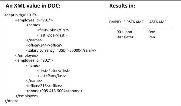
Figure 5-33 XMLTABLE Query output example
The output in Figure 5-34 shows an XML document along with a sample SQL to produce the output in table format.
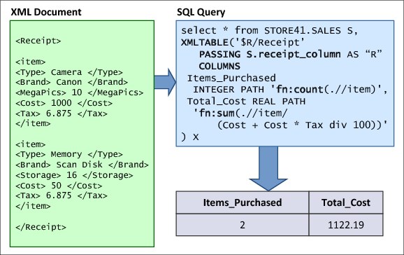
Figure 5-34 Query the total cost of all items that are purchased on each receipt
The SQL/XML support that is included in DB2 for i 7.1 offers a built-in and standardized solution for working with XML from within SQL. XMLTABLE adds significant value by allowing SQL queries to query both XML and relational data in the same query. Working XML data within a relational model is often times a non-trivial task. XMLTABLE offers a high degree of flexibility by supporting a wide range of XPath step expressions, predicates, and built in functions that can be used within the row and column generating expressions.
5.4.32 Run SQL (RUNSQL): A new command
The Run SQL (RUNSQL) command runs a single SQL statement without having to construct a source physical file member or write a program. No spool file is generated. Upon failure, the specific SQL failure message is returned to the command caller.
In other SQL interfaces, an SQL statement is limited to 2 MB in length. The limit on this command is 5000 bytes.
The command has many parameters that are similar to the ones used with the RUNSQLSTM command. RUNSQL runs SQL statements in the invoker's activation group. If RUNSQL is included in a compiled CL program, the activation group of the program is used.
Two examples of using RUNSQL on the command line are shown in Example 5-51. The example also shows how RUNSQL can be used within a CL program.
Example 5-51 Usage of RUNSQL from the command line
RUNSQL SQL(‘INSERT INTO prodLib/work_table VALUES(1, CURRENT TIMESTAMP)')
/* In a CL program, use the Receive File (RCVF) command to read the results of the query */
RUNSQL SQL('CREATE TABLE QTEMP.WorkTable1 AS
(SELECT * FROM qsys2.systables WHERE table_schema = ''QSYS2'') WITH DATA') COMMIT(*NONE) NAMING(*SQL)
Example 5-52 shows how RUNSQL can be used within a CL program. Use the RCVF command if you must read the results of the query.
Example 5-52 Usage of RUNSQL within a CL program
RUNSQL1: PGM PARM(&LIB)
DCL &LIB TYPE(*CHAR) LEN(10)
DCL &SQLSTMT TYPE(*CHAR) LEN(1000)
CHGVAR VAR(&SQLSTMT) +
VALUE(‘DELETE FROM QTEMP.WorkTable1 +
WHERE table_schema = ''' || &LIB || ''‘ ')
RUNSQL SQL(&SQLSTMT) COMMIT(*NONE) NAMING(*SQL)
ENDSQL1: ENDPGM
5.4.33 Native JDBC driver support added for J2SE 7
With the availability of J2SE 7, the native JDBC driver is enhanced to meet the new JDBC 4.1 specification.
The new support for native JDBC on IBM i 7.1 includes:
•java.sql.CallableStatement.getObject(int parameterIndex,java.lang.Class<T>type)
•java.sql.CallableStatement.getObject(java.lang.String parameterName, java.lang.Class<T>type)
•java.sql.Connection.abort(java.util.concurrent.Executor executor)
•java.sql.Connection.setSchema((java.lang.String schema)
•java.sql.Connection.getSchema()
•java.sql.DatabaseMetaData.generatedKeyAlwaysReturned()
•java.sql.DatabaseMetaData.getPseudoColumns(java.lang.String catalog, java.lang.String schemaPattern,
•java.lang.String tableNamePattern,java.lang.String columnNamePattern)
•java.sql.Statement.closeOnCompletion()
•java.sql.Statement.isCloseOnCompletion()
Because the native JDBC driver does not typically use a network connection, the Connection.getNetworkTimeout() and Connection.setNetworkTimeout() methods are not implemented.
5.4.34 QSQPRCED() accepts client special registers
Before this enhancement, the QSQPRCED() Process Extended Dynamic API did not allow the caller direct control over the client special registers. As a result, QSQPRCED() based workloads could not take advantage of client special register branding to improve serviceability.
With this enhancement, the QSQPRCED() SQLP0410 format has been extended to allow any or all of the client special registers to be passed. The new fields are optional and are allowed to vary from one QSQPRCED() call to the next. The values are not bound into the Extended Dynamic SQL package (*SQLPKG). Each client special register value is character data type, varying in length up to a maximum of 255.
QSYSINC/H(QSQPRCED) include details:
typedef struct Qsq_SQLP0410 {
char Function;
char SQL_Package_Name[10];
char Library_Name[10];
char Main_Pgm[10];
char Main_Lib[10];
...
int Cursor_Index; /* @C5A*/
int Statement_Index; /* @C5A*/
int Extended_Cursor_Name_Length; /* @C5A*/
int Extended_Cursor_Name_Offset; /* @C5A*/
int Extended_Statement_Name_Length; /* @C5A*/
int Extended_Statement_Name_Offset; /* @C5A*/
char Concurrent_Access; /* @C8A*/
char Reserved_Space2[15]; /* @C8A*/
int Client_Info_Userid_Length; /* @C9A*/
int Client_Info_Userid_Offset; /* @C9A*/
int Client_Info_Wrkstnname_Length; /* @C9A*/
int Client_Info_Wrkstnname_Offset; /* @C9A*/
int Client_Info_Applname_Length; /* @C9A*/
int Client_Info_Applname_Offset; /* @C9A*/
int Client_Info_Programid_Length; /* @C9A*/
int Client_Info_Programid_Offset; /* @C9A*/
int Client_Info_Acctstr_Length; /* @C9A*/
int Client_Info_Acctstr_Offset; /* @C9A*/
/*char Statement_Data[];*//* Varying length @B5C*/
/*char Extended_User_Defined_Field[]; */
/* CHAR[] @C5A*/
/*char Extended_Statement_Name[];*/
/* CHAR[] @C5A*/
/*char Extended_Cursor_Name[];*/
/* CHAR[] @C5A*/
/*char Client_Info_Userid[];*/
/* CHAR[] @C9A*/
/*char Client_Info_Wrkstnname[];*/
/* CHAR[] @C9A*/
/*char Client_Info_Applname[];*/
/* CHAR[] @C9A*/
/*char Client_Info_Programid_[];*/
/* CHAR[] @C9A*/
/*char Client_Info_Acctstr[];*/
/* CHAR[] @C9A*/
}Qsq_SQLP0410_t;
5.4.35 STRQMQRY command instrumented for client special registers
Similar to RUNSQLSTM, STRSQL, and other database commands, the Start Query Management Query (STRQMQRY) command has been instrumented to use default values for the client special registers. These registers can be used to identify workloads, track usage and more.
Following are the client special register values:
•CURRENT CLIENT_APPLNAME: "START QUERY MANAGEMENT QUERY“
•CURRENT CLIENT_PROGRAMID: "STRQMQRY“
•CURRENT CLIENT_USERID: <actual user ID that called the command>
•CURRENT CLIENT_WRKSTNNAME: <database name>
•CURRENT CLIENT_ACCTNG:- <accounting code of the command user>
These values are used in SQL performance monitors, SQL details for jobs, Visual Explain, and elsewhere within the OnDemand Performance Center.
The Start Database Monitor (STRDBMON) command pre-filters can be used to target STRQMQRY command usage.
5.4.36 QSYS2.QCMDEXC() procedure no longer requires a command length
The QSYS2.QCMDEXC() procedure can be used to run IBM i commands. This enhancement delivers a variant of this procedure where the only parameter passed is the command string. The previous style of QCMDEXC procedure remains valid and supported, but the new version of the QCMDEXC procedure is simpler to use.
The QCMDEXC procedure runs a CL command, where CL-command-string is a character string expression that contains a CL command. The CL-command-string is run as a CL command.
>>-QCMDEXC--(--CL-command-string--)----------------------------><
The schema is QSYS2.
Example 5-53 and Example 5-54 show examples of using the QCMDEXC procedure.
Example 5-53 Using SQL naming, adding a library to the library list
CALL QSYS2.QCMDEXC('ADDLIBLE PRODLIB2'),
Example 5-54 shows adding a library using an expression.
Example 5-54 Using SYSTEM naming, adding a library to the library list using an expression
DECLARE V_LIBRARY_NAME VARCHAR(10);
SET V_LIBRARY_NAME = 'PRODLIB2';
CALL QSYS2/QCMDEXC('ADDLIBLE ' CONCAT V_LIBRARY_NAME);
5.4.37 Adding the ORDERBY parameter to the CPYTOIMPF command
The new (optional) ORDERBY parameter specifies the order of the records that the records are inserted in the file. Here are the ORDERBY parameter values:
•*NONE: No specific order requested. This value is the default value for the command.
•*ARRIVAL: The records are inserted in the order they were inserted in to the file.
•character-value: Specifies an SQL ORDER BY clause that is used for ordering the records in to the file.
The usage of the ORDER BY(*ARRIVAL) parameter and ORDER BY(character-value) examples are shown in Example 5-55, where the Stream File is copied and ordered according to the ORDER BY parameter value.
Example 5-55 Usage of the ORDERBY clause
CPYTOIMPF FROMFILE(CORPDB1/DEPARTMENT) TOSTMF('/iddtdept.file') RCDDLM(*LF) ORDERBY('*ARRIVAL')
CPYTOIMPF FROMFILE(CORPDB1/DEPARTMENT) TOSTMF('/iddtdept.file') RCDDLM(*LF) ORDERBY(' DEPTNO ASC FETCH FIRST 5 ROWS ONLY ')
In addition to the ORDER BY parameter, you can use the following parameters:
•FETCH FIRST n ROWS
•OPTIMIZE FOR n ROWS
•FOR UPDATE
•FOR READ ONLY
•WITH <isolation-level>
•SKIP LOCKED DATA
•USE CURRENTLY COMMITED
•WAIT FOR OUTCOME
5.4.38 System naming convention expanded for permit (/) and (.) qualifiers
Historically, system naming qualification of names required a slash(/) only between the schema-name and the SQL identifier.
Now, when you use system naming, both the slash(/) and dot(.) can be used for object qualification. This change makes it easier to adapt to system naming, as the SQL statement text does not need to be updated.
This enhancement makes it easier to use system naming. Object references can vary and SQL UDFs can now be library qualified with a “.” when you use system naming.
NAMING(*SYS) can be used with (/) and (.), as shown in Example 5-56. However, if the example is used with NAMING(*SQL), it fails.
Example 5-56 Using NAMING(*SYS)
SELECT a.ibmreqd, b.ibmreqd FROM sysibm.sysdummy1 a, sysibm/sysdummy1 b
5.4.39 Direct control of system names for tables, views, and indexes
The FOR SYSTEM NAME clause directly defines the system name for these objects, eliminating the need to run a RENAME after the object is created to replace the system generated name. The name provided in the FOR SYSTEM NAME clause must be a valid system name and cannot be qualified. The first name that is provided for the object cannot be a valid system name.
The optional FOR SYSTEM NAME clause has been added to the following SQL statements:
•CREATE TABLE
•CREATE VIEW
•CREATE INDEX
•DECLARE GLOBAL TEMPORARY TABLE
Use the FOR SYSTEM NAME clause to achieve direct control over table, view, and index system names, making it simpler to manage the database. This support eliminates the need to use the RENAME SQL statement or the Rename Object (RNMOBJ) command after object creation. Additionally, the Generate SQL / QSQGNDDL() interface uses this enhancement to produce SQL DDL scripts that produce identical object names.
When QSQGNDDL() is called using the System_Name_Option = '1', whenever the table, view, or index objects has a system name that differs from the SQL name, the FOR SYSTEM NAME clause is generated. For IBM i Navigator users, you control the System Name Option by selecting the System names for objects option as shown in Figure 5-35.
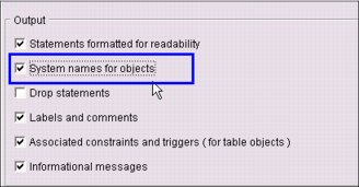
Figure 5-35 Selecting system names for objects
Example 5-57 and Example 5-58 show examples of using the FOR SYSTEM NAME clause.
Example 5-57 COMP_12_11 *FILE object created instead of COMPA00001, COMPA00002, and so on
CREATE OR REPLACE VIEW
PRODLIB/COMPARE_YEARS_2012_AND_2011
FOR SYSTEM NAME COMP_12_11
AS SELECT …
Example 5-58 shows a table with a specific system name.
Example 5-58 Generated table with system name of SALES, instead of generated name CUSTO00001
CREATE TABLE CUSTOMER_SALES FOR SYSTEM NAME SALES (CUSTNO BIGINT…
5.4.40 Modification of global variables within triggers and functions
SQL global variables are a useful construct to achieve session-specific inter-application communication.
Before this change, triggers and functions were allowed to only reference global variables. SQLCODE = -20430 and SQLSTATE = “428GX’ were returned to a trigger or function that attempted to modify a global variable.
Global variables are modified as shown in Example 5-59, which shows the modification of a global variable.
Example 5-59 Usage of a global variable modification
CREATE VARIABLE PRODLIB.MOST_RECENT_ORDER BIGINT DEFAULT 0
CREATE TRIGGER PRODLIB.INSERT_ORDER
BEFORE INSERT ON PRODLIB.ORDER_TABLE
REFERENCING NEW AS N
FOR EACH ROW
MODE DB2ROW
IE:BEGIN ATOMIC
SET PRODLIB.MOST_RECENT_ORDER = NEW_ORDER_VALUE();
SET N.ORDER_VALUE = PRODLIB.MOST_RECENT_ORDER;
END IE
5.4.41 Multiple events supported in a single SQL trigger
Native triggers already can handle INSERT, UPDATE, and DELETE triggering events within a single program. By allowing SQL trigger programs to handle multiple events, the management, installation, and maintenance are improved
A multiple event trigger is a trigger that can handle INSERT, UPDATE, and DELETE triggering events within a single SQL trigger program. The ability to handle more than one event in a single program simplifies management of triggers. In the body of the trigger, the INSERTING, UPDATING, and DELETING predicates can be used to distinguish between the events that cause the trigger to fire. These predicates can be specified in control statements (like IF) or within any SQL statement that accepts a predicate (like SELECT or UPDATE).
For example, the trigger shown in Example 5-60 does the following:
•Increments the number of employees each time a new person is hired
•Decrements the number of employees each time an employee leaves the company
•Raises an error when a salary increase is greater than ten percent
Example 5-60 Multiple events in a trigger
CREATE TRIGGER HIRED
AFTER INSERT OR DELETE OR UPDATE OF SALARY ON EMPLOYEE
REFERENCING NEW AS N OLD AS O FOR EACH ROW
BEGIN
IF INSERTING
THEN UPDATE COMPANY_STATS SET NBREMP = NBREMP + 1;
END IF;
IF DELETING
THEN UPDATE COMPANY_STATS SET NBREMP = NBREMP - 1;
END IF;
IF UPDATING AND (N.SALARY > 1.1 * O.SALARY)
THEN SIGNAL SQLSTATE '75000'
SET MESSAGE_TEXT = 'Salary increase > 10%'
END IF;
END
For more information about multiple events supported in a single SQL trigger, see the following resources:
•SQL Programming Guide
•CREATE TRIGGER SQL statement
•Trigger Event Predicates
5.4.42 New QAQQINI option: SQL_GVAR_BUILD_RULE
This option influences whether global variables must exist when you build SQL procedures, functions, triggers, or running SQL precompiles. Its supported values are:
•*DEFAULT: The default value is set to *DEFER.
•*DEFER: Global variables do not need to exist when an SQL routine is created or the SQL precompiler is run. Because global variables are not required to exist, the create does not fail when an incorrect column name or routine variable is encountered because it is not known at create time whether the name is a global variable. Incorrect name usage results in SQL0206 - “Column or global variable &1 not found.” failures when the statement is run.
•*EXIST: Global variables that are referenced by SQL must exist when the SQL routine is created or the SQL precompiler is run. Using this option, an SQL0206 is issued at create time. This choice is similar to the behavior of previous releases, where incorrect name usage fails at create time with either SQL0312 - “Variable &1 not defined or not usable.” or SQL5001 - “Column qualifier or table &2 undefined”
5.4.43 CPYTOIMPF and CPYFRMIMPF commands include column headings
The CPYTOIMPF and CPYFRMIMPF commands are enhanced with the following features:
•Copy To Import File (CPYTOIMPF): A new (optional) parameter indicates whether the column names should be included as the first row in the target file.
•ADDCOLNAM (*NONE or *SYS or *SQL):
– *NONE: This option is the default. When it is used, the column names are not included.
– *SQL: The column SQL names are used to populate the first row.
– *SYS: The column System names are used to populate the first row.
•Copy From Import File (CPYFRMIMPF): A new (optional) parameter indicates whether the first row should be skipped when you process the import file.
•RMVCOLNAM (*NO or *YES):
– *NO: This option is the default. When it is used, the first row is not skipped.
– *YES: Remove the column names form the file that is being imported by skipping the first row of data.
5.4.44 Improved performance of privileges catalogs and ODBC/JDBC APIs
The performance is improved for the following items.
•JDBC: DatabaseMetaData.getColumnPrivileges() and DatabaseMetaData.getTablePrivileges()
•SQL CLI and ODBC: SQLColumnPrivileges() and SQLTablePrivileges()
•DB2 for i Catalogs in SYSIBM: Variable_Privileges, Usage_Privileges, Routine_Privileges, UDT_Privileges, SQLTablePrivileges, and SQLColPrivileges
The SQL in Example 5-61 produces the output that is shown in Figure 5-36, which clearly shows the privileges by GRANTEE over the selected schema and table.
Example 5-61 Who is allowed to modify this table
SELECT GRANTEE, PRIVILEGE FROM SYSIBM.SQLTablePrivileges
WHERE TABLE_SCHEM = ‘PRODLIB’ AND
TABLE_NAME = ‘DEPARTMENT’ AND
PRIVILEGE IN (‘UPDATE’,’INSERT’,’DELETE’)
ORDER BY GRANTEE
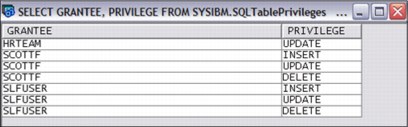
Figure 5-36 List of users with their relevant privileges
5.4.45 Show statements: Index creates and statistics advised
These two new columns appear when show statements are used against a plan cache snapshot or SQL performance monitor. These two new columns do not require a System i Navigator update. The two new columns can be added to your view by clicking Columns in the SQL Plan Cache Snapshots window, as shown in Figure 5-37.
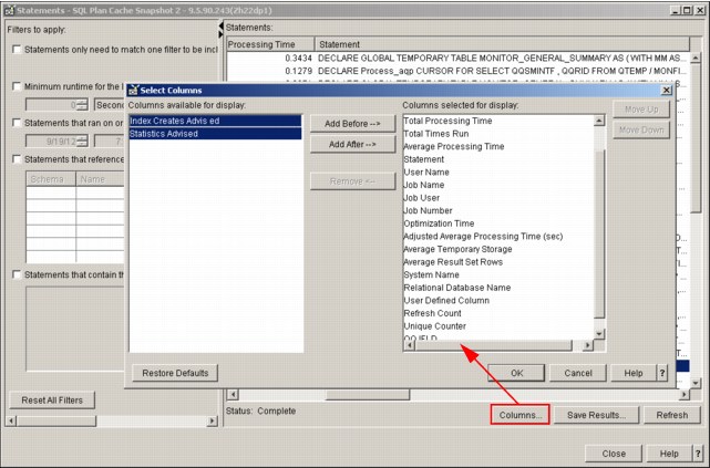
Figure 5-37 Two new columns available for show statements
5.4.46 The RUNSQLSTM command and the OPTION parameter
The OPTION parameter of RUNSQLSTM provides direct control over the command output file. There is no unnecessary spool file accumulation.
The values for the OPTION parameter are:
•*LIST (default): A complete listing with the contents of the source and all errors is generated.
•*NOSRC: A listing with only the messages is generated.
•*ERRLIST: A complete listing is generated only if errors greater than the ERRLVL parameter are encountered during processing.
•*NOLIST: No listing is generated. If errors greater than the ERRLVL parameter are encountered during processing, the messages are sent to the job log.
Running the statement as shown in Example 5-62 obtains a complete listing only if errors greater than the ERRLVL parameter are encountered during processing.
Example 5-62 Obtaining a complete listing
RUNSQLSTM SRCFILE(CLIVEG/QSQLSRC) SRCMBR(STA1) OPTION(*ERRLIST)
An example output of *ERRLIST is shown in Figure 5-38.
|
Record *...+... 1 ...+... 2 ...+... 3 ...+... 4 ...+... 5 ...+... 6 ...+... 7
1 SELECT * FROM GRIFFIC/CUSTOMER;
* * * * * E N D O F S O U R C E * * * * *
5770SS1 V7R1M0 100423 Run SQL Statements STA1
Record *...+... 1 ...+... 2 ...+... 3 ...+... 4 ...+... 5 ...+... 6 ...+... 7
MSG ID SEV RECORD TEXT
SQL0084 30 1 Position 1 SQL statement not allowed.
Message Summary
Total Info Warning Error Severe Terminal
1 0 0 0 1 0
30 level severity errors found in source
* * * * * E N D O F L I S T I N G * * * *
|
Figure 5-38 *ERRLIST output highlighting error details
5.4.47 Improved NULLID package management
NULLID package management automates the creation of necessary objects (collections and dynamic packages) to more seamlessly allow applications using DB2 family database connectivity methods to access data in DB2 for i.
DB2 for Linux, UNIX, and Windows, IBM DB2 Universal Driver for SQLJ and JDBC, ODBC, CLI, IBM DB2 Connect™, and other application requesters rely upon SQL package (*SQLPKG) objects within the NULLID collection.
The NULLID enhancements include:
•The NULLID collection is created automatically upon the first attempt by a DRDA client to bind or run using a package within NULLID.
•The ownership of the NULLID collection is assigned to the QSYS user profile and *PUBLIC is granted *CHANGE authority by default when the system automatically creates the NULLID collection.
•DB2 for i also automatically creates the dynamic packages that are used by JDBC, ODBC, and CLI. These packages are named SYSzcxy, SYSzcxyy, and SYSzTAT.
Before you use these clients to access data on IBM i, you must create IBM i SQL packages for these application programs.
5.4.48 Java stored procedures and functions: System naming option
The Native JDBC driver is enhanced to include a new method to allow the specification of system naming.
The method can be used to turn system naming mode ON and OFF. To use this method, an appropriate cast of the java.sql.Connection object must be made to the com.ibm.db2.jdbc.DB2Connection class.
Before you exit the method, the method returns the connection to the default value. Failure to do so might cause unexpected behavior in other Java stored procedure and Java user-defined functions.
Example 5-63 shows an example of how system naming is enabled in a Java stored procedure.
Example 5-63 How system naming can be enabled in a Java stored procedure
---------------------------------------------------------------------------------
Parameter style DB2GENERAL:
---------------------------------------------------------------------------------
DB2Connection connection = (DB2Connection) getConnection();
connection.setUseSystemNaming(true);
....
.... do work using the connection
....
connection.setUseSystemNaming(false);
---------------------------------------------------------------------------------
Parameter style JAVA:
---------------------------------------------------------------------------------
DB2Connection connection = (DB2Connection) DriverManager.getConnection("jdbc:default:connection");
connection.setUseSystemNaming(true);
....
.... do work using the connection
....
connection.setUseSystemNaming(false);
Before you exit the method, the method returns the connection to the default value. Failure to do so might cause unexpected behavior in other Java stored procedure and Java user-defined functions
Use *LIBL (Library List) in Java procedures and functions.
5.4.49 Named arguments and defaults for parameters: Procedures
There are some enhancements to the named arguments and defaults for parameters on procedures:
•Named and default parameters are supported for SQL and external procedures that make it possible to run more SQL applications on IBM i.
•You can extend procedures without fear of breaking existing callers and simplify the calling requirements by adding default values.
•Procedure call invocation has the same type of support as CL commands.
With this enhancement:
•Parameters can be omitted if the routine was defined with a default value.
•Parameters can be specified in any order by specifying the name in the call.
•This enhancement works with LANGUAGE SQL and EXTERNAL procedures.
Usage of the named arguments and default parameters is shown in Example 5-64.
Example 5-64 Parameter usage
CREATE PROCEDURE p1 (i1 INT, i2 INT DEFAULT 0, i3 INT DEFAULT -1)...
CALL p1(55)
CALL p1(55, i3=>33)
Figure 5-39 shows the DEFAULT clause and its options.
Figure 5-39 The default clause
5.4.50 Improved catalog management for procedures and functions
When an SQL or external procedure or function is created, the routine information is stored within the *PGM or *SRVPGM. Previously, when Librarian commands were used to copy, move, or rename the object, the QSYS2/SYSROUTINE, SYSPARMS, and SYSRTNDEP catalogs were left unchanged.
The following commands (and their API counterparts) were changed to keep the catalogs in sync with the executable object for procedures and functions:
•Create Duplicate Object (CRTDUPOBJ): The routine catalog information is duplicated and the SYSROUTINE EXTERNAL_NAME column points to the newly duplicated executable object.
•Copy Library (CPYLIB): The routine catalog information is duplicated and the SYSROUTINE EXTERNAL_NAME column points to the newly duplicated executable object.
•Rename Object (RNMOBJ): The routine catalog information is modified with the SYSROUTINE EXTERNAL_NAME column, which points to the renamed executable object.
•Move Object (MOVOBJ): The routine catalog information is modified with the SYSROUTINE EXTERNAL_NAME column, which points to the moved executable object
There is coverage for Librarian APIs or other operations that are built upon these commands.
The changed behavior can be partially disabled by adding an environment variable. If this environment variable exists, Move Object and Rename Object operations do not update the catalogs. The environment variable has no effect on the CPYLIB and CRTDUPOBJ commands.
Setting the environment variable is shown in Example 5-65.
Example 5-65 Setting the environment variable to partially disable the function
ADDENVVAR
ENVVAR(QIBM_SQL_NO_CATALOG_UPDATE)
LEVEL(*SYS)
5.4.51 SQE enhancement for Encoded Vector Indexes defined with INCLUDE
Taking advantage of the IBM patented EVI indexing technology, and analytics routines using SQL Constructs such as ROLLUP, CUBE, and Grouping Sets, can produce performance benefits.
SQE is enhanced to make Grouping Set queries aware of EVI INCLUDE as an optimization possibility.
Defining an EVI with INCLUDE is shown in the Example 5-66, which also shows an example SQL to query the EVI.
Example 5-66 Encoded Vector Index (EVI) INCLUDE example
CREATE ENCODED VECTOR INDEX GS_EVI01 ON STAR1G.ITEM_FACT
(YEAR ASC, QUARTER ASC, MONTH ASC)
INCLUDE (SUM(QUANTITY),
SUM(REVENUE_WO_TAX),
COUNT(*) )
SELECT YEAR, QUARTER, MONTH, SUM(QUANTITY) AS TOTQUANTITY, SUM(REVENUE_WO_TAX)
FROM ITEM_FACT WHERE YEAR=2012
GROUP BY GROUPING SETS ((YEAR, QUARTER, MONTH),
(YEAR,QUARTER),
(YEAR),
( ))
Fast Index-Only access is possible for CUBE(), ROLLUP(), and GROUPING SETS().
5.4.52 Navigator: System Name column added to show related and all objects
When you use System i Navigator to observe the objects that are related to a table, only the SQL names of those objects appear. The same situation is true when you use the All Objects view under the Schemas folder.
The System i Navigator 7.1 client is enhanced to include the “System Name” column. This information is useful when long names are used and the system name is not obvious, as shown in Figure 5-40.
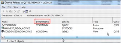
Figure 5-40 System name column included
5.4.53 Navigator – Improved Index Build information
The IBM i Navigator Database Maintenance folder has been enhanced to include two new columns of information:
•Partition: Indexes over a single partition or spanning indexes
•Constraint: Constraint name or NULL
This detail is helpful to fully identify long running index builds for partitioned indexes and constraints. See Figure 5-41.
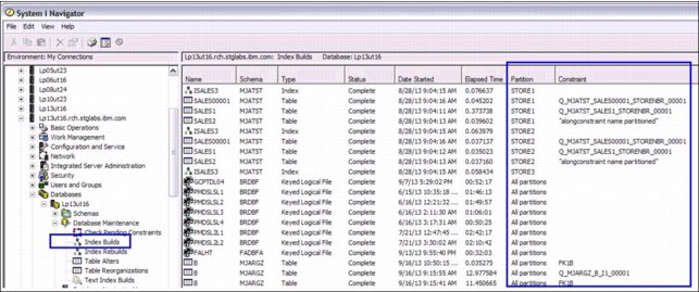
Figure 5-41 Database maintenance index build status
5.4.54 Improved performance for joins over partitioned tables
Before this introduction of this enhancement, data skew (uneven distribution of data values) was not factored in when creating access plans for queries that joined columns in a partitioned table.
This enhancement enables the query statistics engine to detect data skew in the partitioned table if accurate column statistics are available for the partitions. Allowing column level statistics to be automatically collected is the default behavior and a preferred practice.
This enhancement might improve the performance of joins when multiple partitions are queried. An example of multiple partition joins is shown in Example 5-67.
Example 5-67 Multiple partitions join example
Assume the ITEM table (A) contains the product list and the ORDERS table (B) contains sales order details, partitioned by some date range. Several products are particularly heavy sellers, making them skewed in the sales order list.
SELECT B.ITEM NO, SUM(B.QUANTITY) AS Total_Sold
FROM ITEM A LEFT OUTER JOIN ORDERS B ON
A.ITEMNO=B.ITEMNO
GROUP BY B.ITEMNO
ORDER BY TOTAL_SOLD DESC
5.4.55 Navigator: Table list totals
New columns under the Schemas folder now show an aggregate set of information for all members and partitions. You must add these columns by clicking View → Customize this View → Columns. Add the required columns to your view. The following are the new columns:
•Number of rows
•Number of deleted rows
•Partitions
•Size
An example of how to configure your client to show that these new column are shown in Figure 5-42.
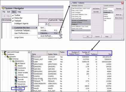
Figure 5-42 Configure your client to show the new columns for tables under the Schemas folder
5.5 DB2 database management and recovery enhancements
This section describes the database management and recovery enhancements to DB2 for i.
5.5.1 Preserving the SQL plan cache size across IPLs
DB2 for i on IBM i 6.1 and 7.1 are enhanced to preserve the SQL Plan Cache size across IPLs and slip installations of the operating system. A scratch installation of the OS resets the SQL Plan Cache size to the default size.
You can explicitly increase the size of the SQL Plan Cache to allow more plans to be saved in the plan cache. This action can improve performance for customers that have many unique queries.
During an IPL, the SQL Plan Cache is deleted and re-created. Before this enhancement, when the plan cache was re-created, it was re-created with the default size of 512 MB, even if you explicitly specified a larger plan cache. Now, the size that is specified by you is preserved and used when it is re-created during any subsequent IPL.
After the latest DB2 Group PTFs are installed, you must change the plan cache size one more time (even if it is changed to the same size as its current size) for the size to be persistently saved.
This CHANGE_PLAN_CACHE_SIZE procedure can be used to change the size of the plan cache. The procedure accepts a single input parameter, that is, the wanted SQL Plan Cache size in megabytes. If the value passed in is zero, the plan cache is reset to its default value. To use the procedure, run the command that is shown in Example 5-68.
Example 5-68 Usage of QSYS2.CHANGE_PLAN_USAGE procedure
CALL qsys2.change_plan_cache_size(1024);
It also possible to get information about Plan Cache properties by using the procedure shown in Example 5-69.
Example 5-69 QSYS2.DUMP_PLAN_CACHE_PROPERTIES
call qsys2.dump_plan_cache_properties('QGPL', 'SQECACHE1'),
select heading,value from qgpl.sqecache1
where heading like '%Time%' ;

select heading,value from qgpl.sqecache1
where heading like '%Time%' ;
5.5.2 Plan cache properties
This section describes enhancements to the SQL plan cache properties, QSYS2.DUMP_PLAN_CACHE_PROPERTIES(). Detail is returned either graphically by using IBM i Navigator or programmatically.
Job scope plan metrics
Job scope plans are a measurement of the use of DECLARED GLOBAL TEMPORARY TABLES (QTEMP). See Figure 5-43.

Figure 5-43 SQL plan cache properties and job scoped plans
Greater insight and control
Following are configuration controls available for use that provide greater plan cache insight and attributes:
•Autosizing enhancement. The ability for the database to automatically adjust the size of the plan cache was first provided in an earlier PTF group. Autosizing relies heavily on measuring and reacting to the hit ratio of the plan cache.
– The hit ratio is defined as the percentage of time that a search of the plan cache by the query optimizer results in finding a plan to use. The default target hit ratio, which was previously set to 70%, is now set to 90% to better reflect more optimal performance, based on customer feedback.
– The maximum size allowed for autosizing, which was previously set to a hard-coded value, is now calculated based on partition size. The more CPUs and storage assigned to a partition, the larger the plan cache is allowed to grow.
– Both the target hit ratio and maximum size are now externalized through the properties and can be adjusted.
|
Note: If the plan cache threshold is explicitly set by the user, autosizing is disabled and is indicated as such with the keyword *DISABLED.
|
•Slowest runs information. For each plan in the plan cache, the database retains information for up to three of the slowest runs of the plan. This value is now externalized through the properties and can be adjusted higher or lower.
•Plan cache activity thresholds. This section shows the highest point for various metrics tracked for either plan cache activity or query activity. These thresholds can be reset (to zero) to restart the threshold tracking. Each threshold has both the high point value and the time stamp when that high point occurred.
•Default values. Default values now show as *DEFAULT or *AUTO, clarifying whether the plan cache threshold is system managed or has been overridden by the user.
•Temporary object storage information. Besides storing the SQL query plans, the plan cache is also used to cache runtime objects so that they can be used across jobs. These runtime objects provided both the executable code for queries and the storage for runtime objects such as hash tables and sorted results. When one job is finished using a runtime object, it is placed in the cache so that another job can pick it up and use it. Two properties are provided which show both the number of these runtime objects cached and the total size of all runtime objects cached in the plan cache.
The following items are customizable:
•Maximum autosize
•Target hit ratio
•Number of longest runs to keep for each query
See Figure 5-44.
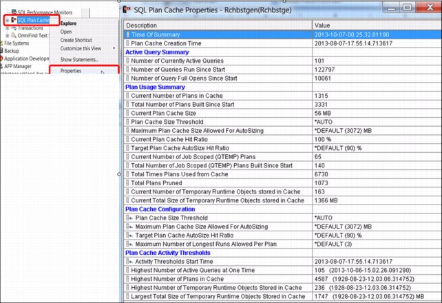
Figure 5-44 Plan cache properties
5.5.3 Prechecking the physical file size during restore
Before this enhancement, when you run a restore of a large physical file, if the available free space on the target ASP was not sufficient to contain the physical file, the restore used all the available storage and caused a system crash. A precheck is now run to ensure that enough storage exists on the target ASP.
5.5.4 Preventing index rebuild on cancel during catch up
When a delayed maintenance index is not open, any changes to rows are recorded, but the update of the index binary tree is delayed until the index is next opened. This action improves the performance of row change operations when the index maintenance is delayed.
Before this enhancement, if a job was canceled while it was opening a delayed maintenance index, the entire index was invalidated and had to be rebuilt from scratch. On large indexes, this operation can be a lengthy operation. This enhancement ensures that in this case that the cancel does not cause the entire index to be invalidated.
5.5.5 QSYS2.SYSDISKSTAT view
The SYSDISKSTAT view can be used to quickly and easily understand disk information using SQL.
Table 5-9 describes the columns in the view. The schema is QSYS2.
Table 5-9 SYSDISKSTAT view
|
Column Name
|
System Column Name
|
Data Type
|
Description
|
|
ASP_NUMBER
|
ASP_NUMBER
|
SMALLINT
|
The independent auxiliary storage pool (IASP) number.
|
|
DISK_TYPE
|
DISK_TYPE
|
VARCHAR(4)
|
Disk type number of the disk.
|
|
DISK_MODEL
|
DISK_MODEL
|
VARCHAR(4)
|
Model number of the disk.
|
|
UNITNBR
|
UNITNBR
|
SMALLINT
|
Unit number of the disk.
|
|
UNIT_TYPE
|
UNIT_TYPE
|
SMALLINT
|
Type of disk unit:
•0 = Not solid-state disk
•1 = Solid-state disk (SSD)
|
|
UNIT_STORAGE_CAPACITY
|
UNITSCAP
|
BIGINT
|
Unit storage capacity has the same value as the unit media capacity for configured disk units. This value is 0 for non-configured units.
|
|
UNIT_SPACE_AVAILABLE
|
UNITSPACE
|
BIGINT
|
Space (in bytes) available on the unit for use.
|
|
PERCENT_USED
|
PERCENTUSE
|
DECIMAL(7,3)
Nullable
|
Percentage that the disk unit has used.
|
|
UNIT_MEDIA_CAPACITY
|
UNITMCAP
|
BIGINT
|
Storage capacity (in bytes) of the unit.
|
|
LOGICAL_MIRRORED_PAIR_STRING
|
MIRRORPS
|
CHAR(1)
Nullable
|
Status of a mirrored pair of disks:
•0 = One mirrored unit of a mirrored pair is not active.
•1 = Both mirrored units of a mirrored pair are active.
•Null if the unit is not mirrored.
|
|
MIRRORED_UNIT_STATUS
|
MIRRORUS
|
CHAR(1)
Nullable
|
Status of a mirrored unit:
•1 = This mirrored unit of a mirrored pair is active (online with current data).
•2 = This mirrored unit is being synchronized.
•3 = This mirrored unit is suspended.
•Contains null if the unit is not mirrored.
|
If you query the UNIT_TYPE field, you can identify information about installed SSD media, as shown in Example 5-70, which shows the relevant SQL to query information for all disks or just for the SSDs.
Example 5-70 Usage of the QSYS2/DISKSTAT catalog for analysis of disk usage
Query information for all disks.
SELECT * FROM QSYS2.SYSDISKSTAT
Query information for all SSD units
SELECT * FROM QSYS2.SYSDISKSTAT WHERE unit_type = 1
5.5.6 STRDBMON: FETCH statement shows failures and warnings
The database monitor accumulates information about fetch requests. The fetch monitor record is written after the cursor is closed. This enhancement tracks the first warning or failure observed during the fetch requests and uses that information about the monitor fetch record.
Here the columns from the monitor that include this information:
•QQI8 (SQLCODE)
•QQC81 (SQLSTATE)
This enhancement enables the use of the STRDBMON FTRSQLCODE() pre-filter as a technique to isolate application fetch-time failures or warnings.
5.5.7 STRDBMON: QQI2 result rows for more statements
Database monitor and SQL performance monitor users can see the number of result rows for DML statements by examining the QQi2 column, where QQRID=1000 (INSERT/UPDATE/DELETE/MERGE).
The monitor support is enhanced to return result rows information for other statements.
Here are some considerations about the number of result rows that are returned for QQI2:
•SQL DML statements (INSERT, UPDATE, DELETE, or MERGE) show the total number of rows that are changed.
•CREATE TABLE AS and DECLARE GLOBAL TEMPORARY TABLE with the WITH DATA parameter shows the total number of rows that are inserted into the table.
•Any other query-based statement shows the estimated number of rows for the resulting query.
•All remaining statements show either -1 or 0.
5.5.8 Adding result set information to QUSRJOBI() and Systems i Navigator
Two new fields are returned by QUSRJOBI() and SQL Details for jobs:
•Available result sets: Shows the number of result sets that are currently available to the job.
•Unconsumed result sets: Shows the cumulative number of result sets in the job that were not used by the calling program and were discarded by the system.
The two new result sets returned by QUSRJOBI() are displayed in IBM i Navigator within the SQL details for jobs, as shown in Figure 5-45.
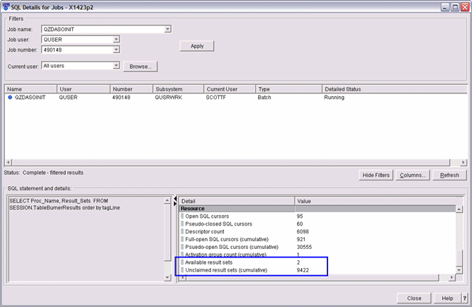
Figure 5-45 Two new result sets returned by QUSRJOBI() displayed in SQL details for jobs
5.5.9 STRDBMON pre-filtering of QUERY/400 command usage
Query/400 commands Run Query (RUNQRY), Work With Queries (WRKQRY), and Start Query (STRQRY) generate database monitor records. This enhancement can easily identify Query/400 users and the queries run through the Filter by Client Program database monitor pre-filter.
STRQRY and WRKQRY activity looks similar to the following output:
QQC21 QQ1000
QR QUERY/400 LIBRARY/FILENAME.MBRNAME
QR QUERY/400 LIBRARY/FILENAME.MBRNAME
RUNQRY activity looks similar to the following output:
QQC21 QQ1000
QR RUNQRY CLIVEG/QUERY1
QR RUNQRY CLIVEG/QUERY2
Example 5-71 shows an example of how to run the filter by client program pre-filter.
Example 5-71 Examples of using STRDBMON with the filter by client to identify QUERY/400 usage
IBM i 6.1 Example:
STRDBMON OUTFILE(LIBAARON/QRY400mon)
JOB(*ALL)
COMMENT('FTRCLTPGM(RUNQRY)')
IBM i 7.1 Example:
STRDBMON OUTFILE(LIBAARON/QRY400mon)
JOB(*ALL)
FTRCLTPGM(RUNQRY)
5.5.10 UNIT SSD supported on DECLARE GLOBAL TEMPORARY TABLE
Support was added for the media preference to the DECLARE GLOBAL TEMPORARY TABLE statement. You can place the temporary table directly on to the SSD. The default media preference setting remains UNIT ANY.
The SQL shown in Example 5-72 places the temporary table on the SSD. The existence of this table can be confirmed by using the SQL in Example 5-73. The actual preferences for the table can be identified by the SQL in Example 5-74.
Example 5-72 Placing a global temporary table on to an SSD
DECLARE GLOBAL TEMPORARY TABLE SESSION.TEMP_DAN
(EMPNO CHAR(6) NOT NULL,
SALARY DECIMAL(9, 2),
BONUS DECIMAL(9, 2),
COMM DECIMAL(9, 2))
ON COMMIT PRESERVE ROWS
WITH REPLACE
UNIT SSD
The QSYS2.PARTITION_DISKS table can be queried to determine which media the queried table is on (Example 5-73).
Example 5-73 Determine whether the table is on the SSD
SELECT UNIT_TYPE FROM TABLE(QSYS2.PARTITION_DISKS(‘QTEMP ‘,’TEMP_DAN ‘)) AS X
-- indicates the type of disk unit
-- 0 - Not Solid State Disk (SSD)
-- 1 - Solid State Disk (SSD)
The QSYS2.PARTITION_STATISTICS table can be queried to determine the media preference of the queried table (Example 5-74).
Example 5-74 Determine the media-preference setting for the table
SELECT MEDIA_PREFERENCE FROM
TABLE(QSYS2.PARTITION_STATISTICS(‘QTEMP ‘,’TEMP_DAN ‘)) AS X
--0 - No media preference
--255 - The table should be allocated on Solid State Disk(SSD), if possible.
5.5.11 Adding Maintained Temporary Indexes
The SQL Query Engine is enhanced to use Maintained Temporary Indexes (MTIs) as a source for statistics, which improves the performance of some queries.
The Index Advisor is enhanced to externalize the count (number of times) the MTI is used as a source of statistics and the time stamp of the last time the MTI was used as a source of statistics. This enhancement provides more information that you can use to decide whether to create permanent indexes for MTIs.
Table 5-10 shows the new column definitions for the MTIs.
Table 5-10 MTI column definitions
|
Column name
|
Data type
|
Description
|
|
MTI_USED_FOR_STATS
|
BIGINT
|
The number of times that this specific MTI is used by the optimizer for statistics.
|
|
LAST_MTI_USED_FOR_STATS
|
TIMESTAMP
|
The time stamp that represents the last time that this specific MTI was used by the optimizer to obtain statistics for a query.
|
5.5.12 Adding the QSYS2.REMOVE_PERFORMANCE_MONITOR procedure
DB2 for i Plan Cache snapshots and performance monitors are in physical files and are tracked for System i Navigator users within the QUSRSYS/QAUGDBPMD2 *FILE.
When the DUMP_PLAN_CACHE procedure is called to create an SQL Plan Cache snapshot, a procedure interface is needed to later remove the snapshot file object and any entries for the file object from the System i Navigator tracking table.
REMOVE_PERFORMANCE_MONITOR() accepts two parameters and removes the SQL table matching that name and associated entries from the QUSRSYS/QAUGDBPMD2 *FILE:
•IN FILESCHEMA VARCHAR(10)
•IN FILENAME VARCHAR(10)
SQL Plan Cache snapshots can be maintained by using the CALL statement, as shown in Example 5-75.
Example 5-75 Removing the SQL Plan Cache snapshot and Performance Monitor file
CALL QSYS2.DUMP_PLAN_CACHE(‘CACHELIB',‘NOV2011')
CALL QSYS2.REMOVE_PERFORMANCE_MONITOR(‘CACHELIB',‘MAY2010')
5.5.13 STRDBMON: QQI1 fast delete reason code
When the DELETE SQL statement is used to remove all records from the table in a performance critical environment, you can use the database monitor to understand when fast delete was used and why fast delete did not occur.
The QQI1 column contains this reason code when QQRID=1000 and QQC21='DL'.
The QQI1 values are documented in the IBM i Database Performance and Query Optimization document:
In addition to the monitor support, a CPF9898 diagnostic message appears in the job log and QHST, if either:
•The number of rows in the table is greater than or equal to 100,000.
•The SQL_FAST_DELETE_ROW_COUNT QAQQINI option is set to a non-default value and the # of rows in the table is greater than or equal to that QAQQINI value.
5.5.14 Automatically increasing the SQE Plan Cache size
DB2 for i automatically increases the SQE Plan Cache size unless the plan cache is explicitly set by the user. This enhancement has the following considerations:
•When processing is initiated to remove plans in the cache because of a size constraint, the efficiency rating of the cache is checked. If the rating is too low, the database automatically increases the plan cache size.
•The database auto-sizing does not exceed a certain maximum size.
•The automatic plan cache size decreases the size if the temporary storage on the system exceeds a certain percentage.
•The auto-sized value does not survive an IPL. The default plan cache size is used after an IPL and auto sizing begins again.
•If you explicitly control the plan cache size and want to turn over control of the plan cache size management, set the plan cache size to zero by using the following statement:
CALL qsys2.change_plan_cache_size(0);
5.5.15 Tracking important system limits
A new type of health indicator is available to help you understand when the system is trending towards an outage or serious condition. Automatic tracking of system limits enables you to do the following:
•Understand when an application is trending towards a failure
•Gain insight regarding application or system outages
•Identify applications that are operating inefficiently
•Establish a general use mechanism for communicating limit information
Automatic tracking of important system limits is a new health touchpoint on IBM i. The system instrumentation for automated tracking focuses on a subset of the system limits. As those limits are reached, tracking information is registered in a DB2 for i system table called QSYS2/SYSLIMTBL. A view called QSYS2/SYSLIMITS is built over the SYSLIMTBL physical file and provides a wealth of contextual information about the rows in the table.
Example 5-76 provides an example of examining active jobs over time and determining how close you might be coming to the maximum active jobs limit.
Example 5-76 Examining active job levels over time
SELECT SBS_NAME, SIZING_NAME, CURRENT_VALUE, MAXIMUM_VALUE , A.*
FROM QSYS2.SYSLIMITS A
WHERE LIMIT_ID= 19000
ORDER BY CURRENT_VALUE DESC
The output of Example 5-76 on page 270 is shown in Figure 5-46.
Figure 5-46 Example output from the qsys2/syslimits view
Figure 5-47 shows the QSYS2/SYSLIMITS view definition.

Figure 5-47 QSYS2/SYSLIMITS view definition
Table 5-11 shows the QSYS2/SYSLIMTBL table definition.
Table 5-11 QSYS2/SYSLIMTBL table definition
|
SQL long name
|
Field name
|
Data type
|
Description
|
|
LAST_CHANGE_TIMESTAMP
|
LASTCHG
|
TIMESTAMP
|
Timestamp when this row was inserted into the QSYS2/SYSLIMTBL table.
|
|
LIMIT_CATEGORY
|
CATEGORY
|
SMALLINT
|
The category of limit corresponding to this instance of System Limits detail. This smallint value maps to the following categories:
•0 = DATABASE
•1 = JOURNAL
•2 = SECURITY
•3 = MISCELLANEOUS
•4 = WORK MANAGEMENT
•5 = FILE SYSTEM
•6 = SAVE RESTORE
•7 = CLUSTER
•8 =COMMUNICATION
|
|
LIMIT_TYPE
|
LIMTYPE
|
SMALLINT
|
The type of limit corresponding to this instance of System Limits detail. This smallint value maps to the following types:
•1 = OBJECT
•2 = JOB
•3 =SYSTEM
•4 = ASP
|
|
LIMIT_ID
|
|
INTEGER
|
The unique System Limits identifier. The limit identifier values are instrumented within the QSYS2/SQL_SIZING table, in the SIZING_ID column. SQL can be used to observe these values. For example:
SELECT SIZING_ID, fSUPPORTED_VALUE, SIZING_NAME, COMMENTS
FROM QSYS2.SQL_SIZING
ORDER BY SIZING_ID DESC
|
|
JOB_NAME
|
|
VARCHAR(28)
|
The name of the job when the instance of System Limits detail was logged.
|
|
USER_NAME
|
CURUSER
|
VARCHAR(10)
|
The name of the user in effect when the instance of System Limits detail was logged.
|
|
CURRENT_VALUE
|
CURVAL
|
BIGINT
|
The current value of the System Limits detail.
|
|
SYSTEM_SCHEMA_NAME
|
SYS_NAME
|
VARCHAR(10)
|
The library name for this instance of System Limits detail, otherwise this is set to NULL.
|
|
SYSTEM_OBJECT_NAME
|
SYS_ONAME
|
VARCHAR(30)
|
The object name for this instance of System Limits detail, otherwise this is set to NULL.
|
|
SYSTEM_TABLE_MEMBER
|
SYS_MNAME
|
VARCHAR(10)
|
The member name for an object limit specific to database members, otherwise this is set to NULL.
|
|
OBJECT_TYPE
|
OBJTYPE
|
VARCHAR(7
|
This is the IBM i object type when an object name has been logged under the SYSTEM_SCHEMA_NAME and SYSTEM_OBJECT_NAME columns. When no object name is specified, this column is set to NULL.
|
|
ASP_NUMBER
|
ASPNUM
|
SMALLINT
|
Contains NULL or the ASP number related to this row of System Limits detail.
|
5.5.16 DB2 for i Services
Table 5-12 on page 273 provides a list of the DB2 for i Services available. For the most current list of services, see the following website:
Table 5-12 DB2 for i services
|
DB2 for i service
|
Type of service
|
Reference for more information
|
|
PTF Services
|
||
|
QSYS2.PTF_INFO
|
View
|
|
|
QSYS2.GROUP_PTF_INFO
|
View
|
|
|
Security Services
|
||
|
QSYS2.USER_INFO
|
View
|
|
|
QSYS2.FUNCTION_INFO
|
View
|
|
|
QSYS2.FUNCTION_USAGE
|
View
|
|
|
QSYS2.GROUP_PROFILE_ENTRIES
|
View
|
|
|
QSYS2.SQL_CHECK_AUTHORITY()
|
UDF
|
|
|
QSYS2.SET_COLUMN_ATTRIBUTE()
|
Procedure
|
|
|
Work Management Services
|
||
|
QSYS2.SYSTEM_VALUE_INFO
|
View
|
|
|
QSYS2.GET_JOB_INFO()
|
UDTF
|
|
|
TCP/IP Services
|
||
|
SYSIBMADM.ENV_SYS_INFO
|
View
|
|
|
QSYS2.TCPIP_INFO
|
View
|
|
|
Storage Services
|
||
|
QSYS2.USER_STORAGE
|
View
|
|
|
QSYS2.SYSDISKSTAT
|
View
|
|
|
Object Services
|
||
|
QSYS2.OBJECT_STATISTICS()
|
UDTF
|
|
|
System Health Services
|
||
|
QSYS2.SYSLIMTBL
|
Table
|
|
|
QSYS2.SYSLIMITS
|
View
|
|
|
Journal Services
|
||
|
QSYS2.DISPLAY_JOURNAL()
|
UDTF
|
|
|
Application Services
|
||
|
QSYS2.QCMDEXC()
|
Procedure
|
|
The following sections provide details for those DB2 for i services that are not previously covered in this document
QSYS2.SYSTEM_VALUE_INFO view
The SYSTEM_VALUE_INFO view returns the names of system values and their values. The list of system values can be found in the Retrieve System Values (QWCRSVAL) API. For more information about the QWCRSVAL API, see the following website:
You must have *ALLOBJ or *AUDIT special authority to retrieve the values for QAUDCTL, QAUDENDACN, QAUDFRCLVL, QAUDLVL, QAUDLVL2, and QCRTOBJAUD. The current value column contains ‘*NOTAVL’ or -1 if accessed by an unauthorized user.
Table 5-13 describes the columns in the view. The schema is QSYS2.
Table 5-13 SYSTEM_VALUE_INFO view
|
Column Name
|
System Column Name
|
Data Type
|
Description
|
|
SYSTEM_VALUE_NAME
|
SYSVALNAME
|
VARCHAR(10)
|
Name of the system value.
|
|
CURRENT_NUMERIC_VALUE
|
CURNUMVAL
|
BIGINT
|
Contains a value if the system value is numeric data, otherwise, contains a null value.
|
|
CURRENT_CHARACTER_VALUE
|
CURCHARVAL
|
VARGRAPHIC(1280)
CCSID(1200)
|
Contains a value if the system value is character data, otherwise, contains a null value.
|
The following statement examines the system values that are related to maximums:
SELECT * FROM SYSTEM_VALUE_INFO
WHERE SYSTEM_VALUE_NAME LIKE '%MAX%'
Which returns the following information:
SYSTEM_VALUE_NAME CURRENT_NUMERIC_VALUE CURRENT_CHARACTER_VALUE
QMAXACTLVL 32,767 -
QMAXSIGN - 000005
QPWDMAXLEN 8 -
QMAXSGNACN - 3
QMAXJOB 163,520 -
QMAXSPLF 9,999 -
QSYS2.USER_STORAGE view
The USER_STORAGE view contains details about storage by user profile. The user storage consumption detail is determined by using the Retrieve User Information (QSYRUSRI) API. For more information about the QSYRUSRI API, see the following website:
The following are details about the USER_STORAGE view:
•You must have *READ authority to a *USRPRF or information is not returned.
•User storage is broken down by SYSBAS and iASPs.
•To see information for independent ASPs (iASPs), the iASP must be varied on.
Table 5-14 describes the columns in the view. The schema is QSYS2.
Table 5-14 User_storage view
|
Column Name
|
System Column Name
|
Data Type
|
Description
|
|
AUTHORIZATION_NAME
|
USER_NAME
|
VARCHAR(10)
Nullable
|
User profile name.
|
|
ASPGRP
|
ASPGRP
|
VARCHAR(10)
Nullable
|
Name of the independent ASP or *SYSBAS.
|
|
MAXIMUM_STORAGE_ALLOWED
|
MAXSTG
|
BIGINT
Nullable
|
Maximum amount of auxiliary storage (in kilobytes) that can be assigned to store permanent objects owned by the user. Contains null if the user does not have a maximum amount of allowed storage.
|
|
STORAGE_USED
|
STGUSED
|
BIGINT
Nullable
|
Amount of auxiliary storage (in kilobytes) occupied by the user's owned objects for this ASPGRP.
|
The following example shows determining how much storage user SCOTTF has consumed:
SELECT * FROM QSYS2/USER_STORAGE
WHERE USER_NAME = ‘SCOTTF’
Figure 5-48 shows the output from this example.
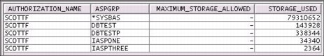
Figure 5-48 USER_STORAGE example output
5.5.17 DISPLAY_JOURNAL (easier searches of Audit Journal)
Displaying a journal entry from a GUI interface today requires using APIs or writing the journal entries to an outfile. The APIs are labor-intensive and the outfile is somewhat restrictive and slower because a copy of the data required.
QSYS2/DISPLAY_JOURNAL is a new table function that allows the user to view entries in a journal by running a query. There are many input parameters of the table function that can be used for best performance to return only those journal entries that are of interest.
For more information about the special values, see the Retrieve Journal Entries (QjoRetrieveJournalEntries ) API in the IBM i 7.1 Knowledge Center. Unlike many other UDTFs in QSYS2, this one has no DB2 for i provided view.
The following is a brief summary of the parameters:
•Journal_Library and Journal_Name
The Journal_Library and Journal_Name must identify a valid journal. *LIBL and *CURLIB are NOT allowed as a value of Journal_Library.
•Starting_Receiver_Library and Starting_Receiver_Name
If the specified Starting_Receiver_Name is the null value, an empty string, or a blank string, *CURRENT is used and the Starting_Receiver_Library is ignored.
If the specified Starting_Receiver_Name contains the special values *CURRENT, *CURCHAIN, or *CURAVLCHN, the Starting_Receiver_Library is ignored.
Otherwise, the Starting_Receiver_Name and Starting_Receiver_Library must identify a valid journal receiver.
*LIBL and *CURLIB can be used as a value of the Starting_Receiver_Library.
The ending journal receiver cannot be specified and is always *CURRENT.
•Starting_Timestamp
If the specified Starting_Timestamp is the null value, no starting time stamp is used. A value for Starting_Timestamp and Starting_Sequence cannot be specified at the same time. However, both values can be queried when querying the table function.
•Starting_Sequence
If the specified Starting_Sequence is the null value, no starting sequence number is used. If the specified Starting_Sequence is not found in the receiver range, an error is returned. A value for Starting_Timestamp and Starting_Sequence cannot be specified at the same time. However, both values can be queried when querying the table function.
•Journal_Codes
If the specified Journal_Codes is the null value, an empty string, or a blank string, *ALL is used. Otherwise, the string can consist of the special value *ALL, the special value *CTL, or a string that contains containing one or more journal codes. Journal codes can be separated by one or more separators. The separator characters are the blank and comma. For example, a valid string can be 'RJ' or 'R J' or 'R,J' or 'R, J'.
•Journal_Entry_Types
If the specified Journal_Entry_Types is the null value, an empty string, or a blank string, *ALL is used. Otherwise, the string can consist of the special value *ALL, the special value *RCD, or a string that contains one or more journal entry types. Journal entry types can be separated by one or more separators. The separator characters are the blank and comma. For example, a valid string can be 'RJ' or 'R J' or 'R,J' or 'R, J'.
•Object_Library, Object_Name, Object_ObjType, and Object_Member
If the specified Object_Name is the null value, an empty string, or a blank string, no object name is used and the Object_Library, Object_ObjType, and Object_Member are ignored.
If the specified Object_Name contains the special value *ALL, Object_Library must contain a library name and Object_ObjType must contain a valid object type (for example, *FILE).
Otherwise:
– Only one object can be specified and the Object_Library, Object_Name, Object_ObjType, and Object_Member must identify a valid object.
– *LIBL and *CURLIB can be used as a value of the Object_Library.
– The Object_ObjType must be one of *DTAARA, *DTAQ, *FILE, or *LIB (*LIB is version 6.1 only).
– The Object_Member can be *FIRST, *ALL, *NONE, or a valid member name. If the specified object type was not *FILE, the member name is ignored.
•User
If the specified User is the null value, or an empty string or a blank string, *ALL is used. Otherwise, you must identify a valid user profile name.
•Job
If the specified Job is the null value, or an empty string, or a blank string, *ALL is used. Otherwise, the Job must identify a valid job name of a specific job where the first 10 characters are the job name, the second 10 characters are the user name, and the last 6 characters are the job number.
•Program
If the specified Program is the null value, an empty string, or a blank string, *ALL is used. Otherwise, the Program must identify a valid program name.
See Example 5-77 for an example of querying a data journal.
Example 5-77 Querying a data journal
set path system path, mjatst; -- Change mjatst to your library you chose above
-- Select all entries from the *CURRENT receiver of journal mjatst/qsqjrn.
select * from table (
Display_Journal(
'MJATST', 'QSQJRN', -- Journal library and name
'', '', -- Receiver library and name
CAST(null as TIMESTAMP), -- Starting timestamp
CAST(null as DECIMAL(21,0)), -- Starting sequence number
'', -- Journal codes
'', -- Journal entries
'','','','', -- Object library, Object name, Object type, Object member
'', -- User
'', -- Job
'' -- Program
) ) as x;
Figure 5-49 shows the results of Example 5-77 on page 277.
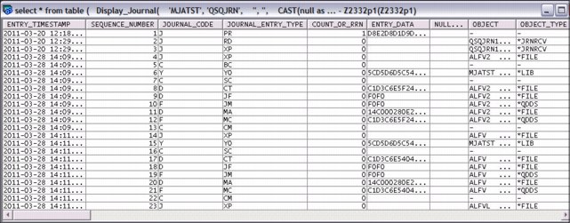
Figure 5-49 Displaying journal data
These are enhancements to the security audit journal (QAUDJRN):
•Search capability for object names
•New columns to identify the object:
– Library objects:
• OBJECT_SYSTEM_SCHEMA
• OBJECT_SYSTEM_NAME
• MEMBER_NAME
• OBJECT_ASP_NUMBER
• OBJECT_ASP_DEVICE
– DLO objects:
• DLO_NAME
• FOLDER_PATH
– IFS objects:
• PARENT_FILE_ID
• OBJECT_FILE_ID
• RELATIVE_DIRECTORY_FILE_ID
• OBJECT_FILE_NAME
• PATH_NAME
• OBJECT_ASP_NUMBER
• OBJECT_ASP_DEVICE
These are enhancements for data journals:
•Search capability for IFS names
•New columns to identify the object:
– Journal code B:
• PARENT_FILE_ID
• OBJECT_FILE_ID
• RELATIVE_DIRECTORY_FILE_ID
• OBJECT_FILE_NAME
• PATH_NAME
• OBJECT_ASP_NUMBER
• OBJECT_ASP_DEVICE
– Object type *STMF, *DIR, or *SYMLINK:
• OBJECT_FILE_ID
• RELATIVE_DIRECTORY_FILE_ID
• PATH_NAME
Example 5-78 shows an example of querying a data journal using filtering criteria to find changes made by SUPERUSER against the PRODDATA/SALES table.
Example 5-78 Query a data journal using filtering criteria
select journal_code, journal_entry_type, object, object_type, X.* from table (
QSYS2.Display_Journal(
'PRODDATA', 'QSQJRN', -- Journal library and name
'', '', -- Receiver library and name
CAST(null as TIMESTAMP), -- Starting timestamp
CAST(null as DECIMAL(21,0)), -- Starting sequence number
'', -- Journal codes
'', -- Journal entries
'PRODDATA','SALES','*FILE','SALES', -- Object library, Object name, Object type, Object member
'', -- User
'', -- Job
'' -- Program
) ) as x
WHERE journal_entry_type in ('DL', 'PT','PX', 'UP') AND "CURRENT_USER" = 'SUPERUSER'
order by entry_timestamp desc
Figure 5-50 shows the results of the query in Example 5-78.
Figure 5-50 Data journal queried by object
5.5.18 IBM i Navigator improved ability to mine journals
IBM i Navigator has been enhanced to make it easier to analyze audit and data journals.
Following are enhancements to improve the ability to mine the security audit journal (QAUDJRN):
•New default columns displayed
•New columns to identify the object
•Search capability for object names based on names in the Entry Specific Data Object type
•Generic library name
•Generic file name
•Search capability for IFS names (or any other column) available in the Additional filters box
Figure 5-51 shows using IBM i Navigator to view security audit journal (QAUDJRN) data.
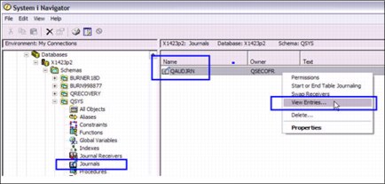
Figure 5-51 Using IBM i Navigator to view security audit journal (QAUDJRN) data
Following are enhancements to improve the ability to mine data journals:
•New default columns displayed
•New columns to identify the IFS objects
•Search capability for object names based on Journal ID (existing support)
•Search capability for IFS names (or any other column) available in the Additional filters box
Figure 5-52 shows using IBM i Navigator to view data journals.
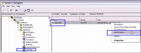
Figure 5-52 Using IBM i Navigator to view data journals
Figure 5-53 shows a graphical alternative to using the DISPLAY_JOURNAL user-defined table function. In this example, IBM i Navigator is used to do journal data dynamic filtering and improved journal data segregation. This alternative makes it easy to work with entries, reorder columns, and understand entry-specific data.

Figure 5-53 Journal data dynamic filtering and improved journal data segregation
On the Journal Viewer window, click Columns to see the columns available for display and to be able to add new columns. See Figure 5-54.
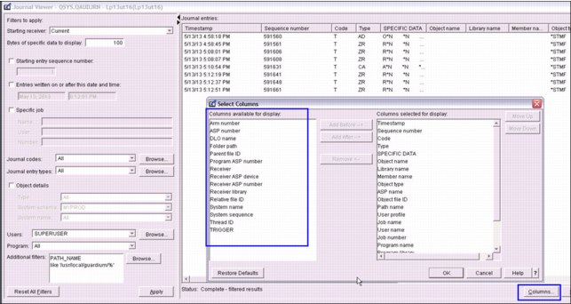
Figure 5-54 IBM i Navigator columns customization
5.5.19 Navigator for i: A new look and no client to manage
You can use the new look for IBM Navigator for i to perform enhanced database management without client software to manage. The following are some of the enhanced functions:
•A new dynamic navigation area allows for easy navigation to folders and areas in the database.
•New tab support provides improved object list viewing and interaction.
•There is improved performance and fewer clicks to reach endpoints.
•New database capabilities include procedure/function creation/definition and view/edit table contents.
An advanced drill-down using the new look of IBM Navigator for i is shown in Figure 5-55.

Figure 5-55 Enhanced drill-down using the new look of IBM Navigator for i
5.6 DB2 for Web Query for i (5733-QU2, 5733-QU3, and 5733-QU4)
DB2 Web Query for i consists of a foundation product, 5733-QU2, and two more optional products, 5733-QU3, and 5733-QU4. The latest version of these products is Version 1.1.2. IBM introduced a packaging option that includes elements from all three of these products into a new bundle called DB2 Web Query for i Standard Edition.
5.6.1 DB2 Web Query for i (5733-QU2)
This product provides several easy to use, web-based tools for building reports and Business Intelligence applications. Report “authors” can choose from Report and Graph Assistant tools that can web enable Query/400 reports or the new InfoAssist report builder that provides a highly intuitive, drag interface for reporting functions. You can build dashboards, integrate data with new or existing spreadsheets, or choose to deliver reports in an analytical form that you can use to slide and dice through the data interactively. DB2 Web Query for i can either be ordered as modules, or you can choose a Standard Edition for a predefined package of components that provide a robust set of components.
The modules are as follows:
•The base module provides the foundation for DB2 Web Query, including the reporting server and the web-based authoring tools. A Query/400 import function allows you to take Query/400 definitions and transform them using the web-based Report Assistant tool. You can use DB2 Web Query to leave your data in DB2 for i and use all security and availability features of the IBM i platform. This base module is priced per processor tier and includes a minimum number of users. Most clients are able to upgrade to the base product at no charge if they own Query/400 and have the latest level of the IBM i software.
•Active Technologies can combine the results of queries and create HTML reports that can be made available to users without needing to be connected to the DB2 for i server. Designed for users “on the go”, the reports contain query results. The data can be viewed in various ways from a browser, including functions to sort, filter the data by different criteria, a calculated field, and chart information for visual impact.
•The DB2 Web Query Developer Workbench feature is an open and intuitive environment that you can use for rapid development of more customized web-based reports and metadata. It includes an HTML layout painter for building dashboards, combining multiple reports into a single view. It is a critical component for developing and managing the metadata that is used to shield the complexities of the database from report authors and users.
•The OLAP Module provides an interactive visualization of the data that you can use to drill down or slice and dice to find trends or exceptions in an analytical process. A single report can be a starting point for complex data analysis. Setting up dimensional definitions in DB2 Web Query Developer Workbench is a prerequisite to using an OLAP report.
•Without Runtime User Enablement, each individual user must be licensed to the base product. With the Runtime User Enablement feature, one or more user licenses can now be defined as a group of runtime only users. If you are familiar with Group Profiles, this concept is a similar concept. Each member of the group is able to run reports concurrently, and each group can contain thousands of users, providing an almost unlimited runtime user licensing model. Users that are defined as runtime users cannot create or edit report definitions, but have full functionality in running reports, including parametrized dashboards, OLAP reports, and more.
•DB2 Web Query Spreadsheet Client provides enhanced capabilities for users of Microsoft Excel. With the Spreadsheet Client, users can create templates or regularly used spreadsheets that can be repopulated with data from DB2 for i (or Microsoft SQL Server with the following noted adapter feature). Users with the appropriate authority can start the Report Assistant component of the BASE product to build their own query to populate spreadsheet cells. Data computations and totals are brought into Excel as native formulas, and you can add data filtering and style the output to further enhance the data within Excel.
•DB2 Web Query Adapter for Microsoft SQL Server provides connectivity from DB2 Web Query to remote SQL server databases. Many IBM i customers have most of their data in DB2 for i, but occasionally want to get real-time access to data in a SQL server database for reporting purposes. The new adapter for SQL server provides access to multiple remote SQL server databases if wanted, and provides seamless access to this data for report authors and users.
•DB2 Web Query Adapter for Oracle JD Edwards allows DB2 Web Query to report on data that is stored in World or EnterpriseOne databases within DB2 for i. The adapter provides a level of seamless integration that simplifies authoring of reports. The adapter also preserves data integrity and security during report execution by automatically interfacing to the application’s metadata and security layers.
5.6.2 DB2 Web Query Report Broker (5733-QU3)
This product provides automated report execution and distribution. Use the scheduling facilities to run reports in batch on a daily or weekly basis, on specific dates, or to add blackout dates.
Deliver reports in formats such as PDF, spreadsheet, or other PC file formats and automate report distribution through an email distribution list.
5.6.3 DB2 Web Query Software Developer Kit (5733-QU4)
This product is targeted at application developers. The DB2 Web Query SDK provides a set of web services that you can use to integrate DB2 Web Query functions into applications or to customize an interface into DB2 Web Query or DB2 Web Query Report Broker functions.
The web services allow web applications to authenticate users, view domains and folders, determine report parameters, run DB2 Web Query reports, and more. Simplify the programming effort by using the application extension, now part of the SDK. This extension can eliminate the need for programming to the web services and allow you to create a URL interface to report execution that you can embed in an existing or new application.
When you develop using the SDK, the DB2 Web Query BASE product is required and Developer Workbench feature is recommended. Deployment (runtime) environments require the BASE product and the Runtime User Enablement feature of DB2 Web Query.
5.6.4 DB2 Web Query for i Standard Edition
DB2 Web Query, Standard Edition simplifies the decision process of which features to order by including the most popular features in a single package. You can order more features, such as the SQL Server or JDE adapter to the Standard Edition if wanted, but the intent is to combine the most commonly chosen functions into a single order. The DB2 Web Query Standard Edition contains these functions:
•DB2 Web Query for i BASE with the number of users included based on processor group
•Four more User Licenses (that can be used as individual users or as a group of runtime users)
•One PC license of Developer Workbench
•Active Technologies
•OLAP
•Runtime User Enablement
•Spreadsheet Client
•DB2 Web Query Report Broker
•DB2 Web Query Software Developer Kit
5.7 OmniFind Text Search Server for DB2 for i (5733-OMF)
The OmniFind Text Search Server for DB2 for i product available for IBM i 7.1 is enhanced to include more SQL programmable interfaces that extend its support beyond traditional DB2 tables. These interfaces allow text indexing and searching of IBM i objects, such as spool files in an output queue or stream file data in the integrated file system.
A text search collection describes one or more sets of system objects that have their associated text data indexed and searched. For example, a collection might contain an object set of all spool files in output queue QUSRSYS/QEZJOBLOG, or an object set for all stream files in the /home/alice/text_data directory.
The text search collection referred to in this documentation should not be confused with a DB2 schema (sometimes also referred to as a collection), or a Lucene collection (part of the internal structure of a DB2 text search index).
When a text search collection is created, several DB2 objects are created on the system:
•SQL schema with the same name as the collection
•Catalogs for tracking the collection’s configuration
•Catalogs for tracking the objects that are indexed
•SQL Stored procedures to administer and search the collection
•A DB2 text search index for indexing the associated text
Administration of the collection is provided with stored procedures, most of which are created in the schema.
5.7.1 OmniFind for IBM i: Searching Multiple Member source physical files
The OmniFind Text Search Server for DB2 for i product (5733-OMF) for IBM i 7.1 is enhanced to include more SQL programmable interfaces that extend its support beyond traditional DB2 tables.
Multiple Member source physical files are added one at a time to the OmniFind collection. The members from source physical file are retrieved and treated as separate objects.
During the OmniFind update processing, new, changed, or removed members are recognized and processed appropriately.
Two types of instrumentation are available:
•<collection>.ADD_SRCPF_OBJECT_SET (IN SRCPF_LIB VARCHAR(10) CCSID 1208, IN SRCPF_NAME VARCHAR(10) CCSID 1208, OUT SETID INTEGER) CALL UPDATE
•<collection>.ADD_SRCPF_OBJECT_SET (IN SRCPF_LIB VARCHAR(10) CCSID 1208, IN SRCPF_NAME VARCHAR(10) CCSID 1208) CALL UPDATE
For more information about this topic and the OmniFind for i product, see the topic “Searching Spool Files and IFS Stream Files” at developerWorks at:
You can also find updates for OmniFind at:
5.7.2 Navigator for i - Omnifind Collection Management
Within the browser-based version of Navigator for i, controls are available for adding IFS subdirectories and Multiple Member Source Physical Files to a text search collection. See Figure 5-56.
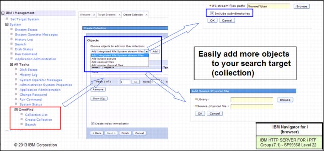
Figure 5-56 Navigator for i improved controls for OmniFind collections
5.8 WebSphere MQ integration
IBM WebSphere® MQ is a family of network communication software products that allow independent and potentially non-concurrent applications on a distributed system to communicate with each other.
The implementation described here provides a set of scalar functions and table functions to provide the integration with DB2.
Scalar functions
The MQREAD function returns a message in a VARCHAR variable from a specified WebSphere MQ location, which is specified by receive-service, using the policy that is defined in service-policy, starting at the beginning of the queue but without removing the message from the queue. If no messages are available to be returned, a null value is returned.
Example 5-79 reads the first message with a correlation ID that matches 1234 from the head of the queue that is specified by the MYSERVICE service using the MYPOLICY policy.
Example 5-79 MQREAD Scalar
SELECT MQREAD ('MYSERVICE','MYPOLICY','1234')
FROM SYSIBM.SYSDUMMY1
The MQREADCLOB function returns a message in a CLOB variable from a specified WebSphere MQ location, which is specified by receive-service, using the policy that is defined in service-policy, starting at the beginning of the queue but without removing the message from the queue. If no messages are available to be returned, a null value is returned.
Example 5-80 reads the first message with a correlation ID that matches 1234 from the head of the queue that is specified by the MYSERVICE service using the MYPOLICY policy.
Example 5-80 MQREADCLOB Scalar
SELECT MQREADCLOB ('MYSERVICE','MYPOLICY','1234')
FROM SYSIBM.SYSDUMMY1
The MQRECEIVE function returns a message in a VARCHAR variable from a specified WebSphere MQ location, which is specified by receive-service, using the policy that is defined in service-policy. This operation removes the message from the queue. If a correlation-id is specified, the first message with a matching correlation identifier is returned. If a correlation-id is not specified, the message at the beginning of queue is returned. If no messages are available to be returned, a null value is returned.
Example 5-81 receives the first message with a correlation-id that matches 1234 from the head of the queue that is specified by the MYSERVICE service using the MYPOLICY policy.
Example 5-81 MQRECEIVE Scalar
SELECT MQRECEIVE ('MYSERVICE','MYPOLICY','1234')
FROM SYSIBM.SYSDUMMY1
The MQRECEIVECLOB function returns a message in a CLOB variable from a specified WebSphere MQ location, which is specified by receive-service, using the policy that is defined in service-policy. This operation removes the message from the queue. If a correlation-id is specified, the first message with a matching correlation identifier is returned. If a correlation-id is not specified, the message at the beginning of queue is returned. If no messages are available to be returned, a null value is returned.
Example 5-82 receives the first message with a correlation-id that matches 1234 from the head of the queue that is specified by the MYSERVICE service using the MYPOLICY policy.
Example 5-82 MQRECEIVECLOB Scalar
SELECT MQRECEIVECLOB ('MYSERVICE','MYPOLICY','1234')
FROM SYSIBM.SYSDUMMY1
If for all of the previously mentioned scalars the receive-service is not specified or the null value is used, the DB2.DEFAULT.SERVICE is used.
The MQSEND function sends the data in a VARCHAR or CLOB variable msg-data to the WebSphere MQ location specified by send-service, using the policy that is defined in service-policy. An optional user-defined message correlation identifier can be specified by correlation-id. The return value is 1 if successful, or 0 if not successful. If the send-service is not specified or the null value is used, the DB2.DEFAULT.SERVICE is used.
On all of these functions, you can specify a correlation-id (correl-id) expression. The value of the expression specifies the correlation identifier that is associated with this message. A correlation identifier is often specified in request-and-reply scenarios to associate requests with replies. The first message with a matching correlation identifier is returned.
Table functions
The MQREADALL function returns a table that contains the messages and message metadata in VARCHAR variables from the WebSphere MQ location that is specified by receive-service, using the policy that is defined in service-policy. This operation does not remove the messages from the queue. If num-rows is specified, a maximum of num-rows messages is returned. If num-rows is not specified, all available messages are returned.
Example 5-83 reads the head of the queue that is specified by the default service (DB2.DEFAULT.SERVICE) using the default policy (DB2.DEFAULT.POLICY). Only messages with a CORRELID of 1234 are returned. All columns are returned.
Example 5-83 MQREADALL table function
SELECT *
FROM TABLE (MQREADALL ()) AS T
WHERE T.CORRELID = '1234'
The MQREADALLCLOB function returns a table that contains the messages and message metadata in CLOB variables from the WebSphere MQ location that is specified by receive-service, using the policy that is defined in service-policy. This operation does not remove the messages from the queue. If num-rows is specified, a maximum of num-rows messages is returned. If num-rows is not specified, all available messages are returned.
Example 5-84 receives the first 10 messages from the head of the queue that is specified by the default service (DB2.DEFAULT.SERVICE), using the default policy (DB2.DEFAULT.POLICY). All columns are returned.
Example 5-84 MQREADALLCLOB table function
SELECT *
FROM TABLE (MQREADALLCLOB (10)) AS T
The MQRECEIVEALL function returns a table that contains the messages and message metadata in VARCHAR variables from the WebSphere MQ location that is specified by receive-service, using the policy that is defined in service-policy. This operation removes the messages from the queue. If a correlation-id is specified, only those messages with a matching correlation identifier are returned. If a correlation-id is not specified, all available messages are returned. If num-rows is specified, a maximum of num-rows messages is returned. If num-rows is not specified, all available messages are returned.
Example 5-85 receives all the messages from the head of the queue that is specified by the service MYSERVICE, using the default policy (DB2.DEFAULT.POLICY). Only the MSG and CORRELID columns are returned.
Example 5-85 MQRECEIVEALL table function
SELECT T.MSG, T.CORRELID
FROM TABLE (MQRECEIVEALL ('MYSERVICE')) AS T
The MQRECEIVEALLCLOB function returns a table that contains the messages and message metadata in CLOB variables from the WebSphere MQ location that is specified by receive-service, using the policy that is defined in service-policy. This operation removes the messages from the queue. If a correlation-id is specified, only those messages with a matching correlation identifier are returned. If correlation-id is not specified, all available messages are returned. If num-rows is specified, a maximum of num-rows messages is returned. If num-rows is not specified, all available messages are returned.
Example 5-86 receives all the messages from the queue that is specified by the default service (DB2.DEFAULT.SERVICE), using the default policy (DB2.DEFAULT.POLICY). The messages and all the metadata are returned as a table.
Example 5-86 MQRECEIVEALLCLOB table function
SELECT *
FROM TABLE (MQRECEIVEALLCLOB ()) AS T
If for all of the previously mentioned table functions the receive-service is not specified or the null value is used, the DB2.DEFAULT.SERVICE is used.
DB2 WebSphere MQ tables
The DB2 WebSphere MQ tables contain service and policy definitions that are used by the DB2 WebSphere MQ functions. The DB2 WebSphere MQ tables are SYSIBM.MQSERVICE_TABLE and SYSIBM.MQPOLICY_TABLE. These tables are user-managed. The tables are initially created by DB2 and populated with one default service (DB2.DEFAULT.SERVICE) and one default policy (DB2.DEFAULT.POLICY). You can modify the attributes of the default service and policy by updating the rows in the tables. You can add more services and policies by inserting more rows in the tables.
DB2 WebSphere MQ CCSID conversion
When a message is sent, the message can be converted to the job CCSID by DB2. When a message is read or received, it can be converted to a specified CCSID by WebSphere MQ.
The msg-data parameter on the MQSEND function is in the job CCSID. If a string is passed for msg-data, it is converted to the job CCSID. For example, if a string is passed for msg-data that has a CCSID 1200, it is converted to the job CCSID before the message data is passed to WebSphere MQ. If the string is defined to be bit data or the CCSID of the string is the CCSID of the job, no conversion occurs.
WebSphere MQ does not run CCSID conversions of the message data when MQSEND is run. The message data that is passed from DB2 is sent unchanged along with a CCSID that informs the receiver of the message and how to interpret the message data. The CCSID that is sent depends on the value that is specified for the CODEDCHARSETID of the service that is used on the MQSEND function. The default for CODEDCHARSETID is -3, which indicates that the CCSID passed is the job default CCSID. If a value other than -3 is used for CODEDCHARSETID, the invoker must ensure that the message data passed to MQSEND is not converted to the job CCSID by DB2, and that the string is encoded in that specified CCSID.
When a message is read or received by a WebSphere MQ scalar or table function, the msg-data return parameter (and the MSG result column for the WebSphere MQ table functions) is also defined in job default CCSID. DB2 does no conversions and relies on WebSphere MQ to perform any necessary conversions. Whether WebSphere MQ converts the message data can be controlled by setting the RCV_CONVERT value to N in the specified policy.
If the specified service has a value for CODEDCHARSETID of -3, DB2 instructs WebSphere MQ to convert any message that is read or received into the job CCSID. If a value other than -3 is used for CODEDCHARSETID, DB2 instructs WebSphere MQ to convert any message that is read or received into that CCSID. Specifying something other than -3 for CODEDCHARSETID in a service that is used to read or receive messages is not a preferred practice because the msg-data return parameter and MSG result column are defined by DB2 in job default CCSID.
When you read or receive a message, truncation can occur. If the specified policy has a value for RCV_ACCEPT_TRUNC_MSG of Y, the message can be truncated without any warning. If the value for RCV_ACCEPT_TRUNC_MSG is N and the message is too long, the function ends with an error.
5.9 DB2 Connect system naming attribute
DB2 Connect V10.1 and IBM i 7.1 have been enhanced to provide naming mode control.
SQL_ATTR_DBC_SYS_NAMING is used on the sqlsetconnectattr() API where:
•SQL_TRUE switches the connection to SYSTEM naming
•SQL_FALSE switches the connection to SQL naming
The sqlsetconnectattr() API can be called before or after a connection is made.
SET PATH = *LIBL can be used to reset the path for system naming use. This support is implemented using a special package flow that is begun at run time.
For more information, see the Call level interface (CLI) driver enhancements topic in the DB2 Knowledge Center:
http://www-01.ibm.com/support/knowledgecenter/SSEPGG_10.1.0/com.ibm.db2.luw.wn.doc/doc/c0055321.html
Example 5-87 shows a typical execution.
Example 5-87 Typical execution
> > > quickc 1 1 sysnam rwpgmr rwp2gmr
> sqlallocstmt 1 1
> sqlsetconnectattr 1 SQL_ATTR_DBC_SYS_NAMING SQL_TRUE
> sqlexecdirec 1 "create schema ashok" -3
> sqlexecdirec 1 "set current schema ashok" -3
> sqlexecdirec 1 "create table ashok/emp1 (id1 int)" -3l
Date and Time Format Controls
DB2 Connect V10.5 and IBM i 6.1 and 7.1 have been enhanced to provide DATE/TIME/DECIMAL format and separator control by supporting environment level and connection level attributes.
•Attribute names:
– SQL_ATTR_DATE_FMT
– SQL_ATTR_DATE_SEP
– SQL_ATTR_TIME_FMT
– SQL_ATTR_TIME_SEP
– SQL_ATTR_DECIMAL_SEP
•Date format values:
– SQL_IBMi_FMT_YMD
– SQL_IBMi_FMT_MDY
– SQL_IBMi_FMT_DMY
– SQL_IBMi_FMT_JUL
– SQL_IBMi_FMT_ISO
– SQL_IBMi_FMT_EUR
– SQL_IBMi_FMT_JIS
– SQL_IBMi_FMT_JOB
•Date separator values:
– SQL_SEP_SLASH
– SQL_SEP_COMMA
– SQL_SEP_PERIOD
– SQL_SEP_BLANK
– SQL_SEP_DASH
– SQL_SEP_JOB
•Time format values:
– SQL_IBMi_FMT_HMS
– SQL_IBMi_FMT_ISO
– SQL_IBMi_FMT_USA
– SQL_IBMi_FMT_EUR
– SQL_IBMi_FMT_JIS
– SQL_IBMi_FMT_JOB
•Time separator values:
– SQL_SEP_COLON
– SQL_SEP_PERIOD
– SQL_SEP_COMMA
– SQL_SEP_BLANK
– SQL_SEP_JOB
•Decimal separator values:
– SQL_SEP_PERIOD
– SQL_SEP_COMMA
– SQL_SEP_JOB
|
Programming Notes: The sqlsetenvattr() API is called before a connection is made, and the sqlsetconnectattr() API can be called before or after a connection is made
|
Example 5-88 shows an example of finding employees with less than two years of tenure.
Example 5-88 Finding employees with less than two years of tenure
sqlsetconnectattr 1 SQL_ATTR_DATE_FMT SQL_IBMi_FMT_EUR
sqlsetconnectattr 1 SQL_ATTR_DATE_SEP SQL_SEP_PERIOD
sqlexecdirect 1 “SELECT EMPNO FROM CORPDATA.EMP
WHERE HIREDATE > ‘09.23.2013‘ – 2 YEARS
ORDER BY LASTNAME, FIRSTNME, MIDINIT" -3
WHERE HIREDATE > ‘09.23.2013‘ – 2 YEARS
ORDER BY LASTNAME, FIRSTNME, MIDINIT" -3
..................Content has been hidden....................
You can't read the all page of ebook, please click here login for view all page.