

IBM i Doctor for IBM i
This appendix describes the changes in IBM iDoctor for IBM i for IBM i 7.1.
The following topics are described:
Installation
The following functions were added to the installation process:
•The save files that are used to install the server builds are now downloaded on demand when running the installation. These can be downloaded through a proxy server if necessary using the settings on the Welcome page of the installation.
•Sending the save files to the IBM i now includes an option to use SSL FTP.
•Validation checks were added for each specified partition to ensure that the partition is able to install iDoctor.
•The default installation directory is now C:Program FilesIBMiDoctor on 32-bit Windows and C:Program Files (x86)IBMiDoctor on 64-bit Windows.
•A check was added for installing Job Watcher at the 6.1 and 7.1 releases to ensure that the Job Watcher definitions file (QAPYJWDFN) exists in QUSRSYS and contains the IBM-supplied definitions.
•In the installation, an option on the Component Selection window that is called Create user profile QIDOCTOR (applies to Base support only) with the default cleared was added.
The iDoctor GUI now requires the Visual Studio 2012 Update 1 or later redistributable package and.NET 4.0 or later. More information about these requirements can be found on the following website:
My Connections View
My Connections View, which is shown in Figure A-1 on page 867, provides the following enhancements:
•Added columns to show access code expiration dates, missing PTFs, ASP group name, and relational database name (if the connection uses an independent ASP).
•New menu options added to Check Expiration Dates or Check PTFs against the wanted partitions. Check PTFs includes checking for the latest Performance Group PTF levels.
•Added menus to Load and Remove all iDoctor Stored Procedures.
•Added Uninstall iDoctor option.
•Added an option to Edit an existing connection.
•Deleted obsolete analysis files for each component.
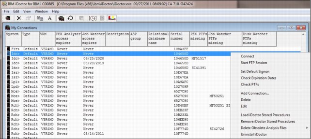
Figure A-1 Options of My Connections View
When you sign on to a system, iDoctor uses the configured sign-on setting defined in System i Navigator (you can access this setting by clicking Properties and clicking the Connection tab for a system). You can use options such as Use Windows user name and password to avoid needing to sign on through iDoctor if your Windows password matches the user name and password of the System i to which you are connecting. iDoctor also uses the System i Access for Windows password cache to avoiding prompting for a password unless needed. If you still want to be prompted for a password every time you start iDoctor, set the Prompt every time option within System i Navigator.
Support was added to view collections that are stored in libraries that are created in Independent ASPs. Use the Add connection menu or Edit menu from the My Connections View to specify the appropriate ASP group name and relational DB name, as shown in Figure A-2. These values cause the QZRCSRVS and QZDASOINIT jobs that are created by iDoctor to recognize data that is stored in the Independent ASP.
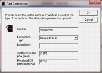
Figure A-2 Add Connection
You can also create connections of type HMC, AIX, or VIOS. Doing so enables appropriate options for each.
Main window
On the main window toolbar, a button was added that enables / disables the display of situational analysis background colors in graphs. A simple click of the button turns it on / off for all graphs (even open ones). Another click of the graph or legend redraws the graph with or without the situations (if found in the data), as shown in Figure A-3.
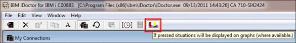
Figure A-3 Button to enable or disable situations analysis background colors
On the main window, which is shown in Figure A-4, the clock icon can now be used from any component to set the preferred time range interval size. The clock icon now has the following additional time grouping options: one-tenth-second, five-second, fifteen-second, five-minute, four-hour, eight-hour, twelve-hour, and twenty-four-hour. The small groupings are useful in PEX Analyzer and the large groupings are useful in Collection Services. More checking was added to the GUI to ensure that only relevant time grouping options are shown for the current data.
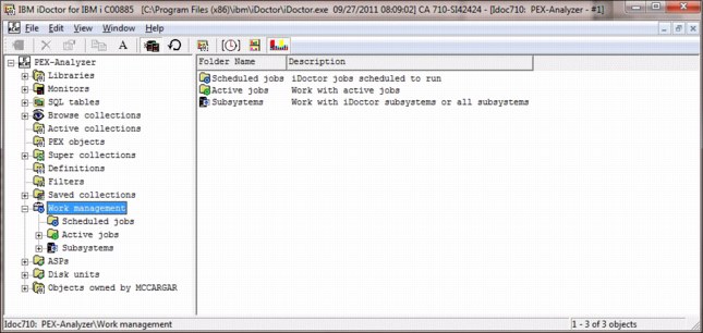
Figure A-4 Main window
You can save a URL for libraries, collections, call stacks, and so on, in iDoctor using the Copy URL menu option or button. The URL can then be pasted into a web browser or saved for future use. The URL shown in Example A-1 opens library COMMON within Job Watcher on system Idoc610.
Example A-1 Opening the COMMON library within Job Watcher on system Idoc610
idoctor:///viewinfo1[type=CFolderLib,sys=Idoc610,lib=COMMON,comp=JW]
All components now provide several common options (folders) for working with data or parts of the system in various ways:
•The Libraries folder displays the libraries on the system that contain data for the current component. You can filter the libraries by owner or library name by using the Filter libraries menu.
•The SQL Tables folder is a repository in iDoctor for working with the tables created by the iDoctor analyses. Comparison options are available by right-clicking more than one SQL table.
•A new Browse Collections option was added that provides alternative ways of looking at the collections that are stored on the system. This function is built from a repository that must be updated periodically by the user using the options that are found when you right-click the Browse Collections folder.
You can use the Browse Collections option to find collections on the system in several ways:
– Partition Name
– Partition Name and VRM
– Partition and collection type
– Library
– Library and collection type
– Collection type
– Collection type and VRM
– VRM
– Month created
– Month created and collection type
Each of the views gives the total size of all collections (in MBs) in each group and the total number, as shown in Figure A-5.

Figure A-5 Browse collections
•Added a Super collections folder that you can use to work with the super collections that exist on the system. These collections contain a folder for each collection type that is collected within the super collection.
•You can use the Saved collections folder to work with any save files that are found on the system that contain iDoctor collections that were saved previously using the iDoctor GUI.
•You can use the Work Management folder to work with scheduled iDoctor jobs, work with active jobs, or work with the subsystems. Within the subsystems folder are options to work the iDoctor subsystems or all subsystems.
The iDoctor components now contain two new folders that show the ASPs and disk units that are configured on the current system. You can use the ASPs folder to drill down to view the disk units within an ASP. The Disk Units folder provides WRKDSKSTS type of statistics with updates provided with each refresh (it also includes total I/O and total sizes), as shown in Figure A-6.
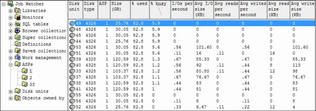
Figure A-6 Overview of the disk status in ASP1
Right-click the Disk Units or ASP folder and click Reset Statistics to restart the collection of disk statistics. You can also use the Select fields menu option when you right-click the folder to rearrange fields or add more fields. The status bar of the main window shows the times for first disk statistics snapshot, and the last one.
Similarly, you find an Active Jobs (see Figure A-4 on page 868) folder on the same window, which provides WRKACTJOB-like function from the iDoctor client, as shown in Figure A-7. You can also sort by a statistic and refresh to keep tabs on the top processor users, and so on. There is also a filter option to filter the list by name, user, number, current user, or minimum processor percentage. Click the Select fields menu option when you right-click the folder to rearrange fields or add more fields. Expanding a job shows the threads and the thread statistics available for each job. You can start Job Watcher or PEX Analyzer collections or add Job Watcher / PEX definitions using the selected jobs within the Active jobs folder. You can also end the selected jobs or view job logs.

Figure A-7 Overview of Active Jobs (WRKACTJOB)
You can use the objects that are owned by a user folder to manage (view / delete) the objects on the system that are owned by the current user. This function is primarily intended to aid in disk space cleanup and options are provided to view only iDoctor objects, or all objects that are owned by the current user.
Collection options
The Collection menu now contains an Analyses menu for all components. Choosing an option under this menu runs a program that creates SQL tables that are needed for further analysis. In most cases, more reports become available after the analysis completes and the collection is refreshed (by pressing F5.)
The Summarize menu option in CSI and Job Watcher moved to Analyses - Run Collection Summary. Choosing this option now displays a window that you can use to filter the collection data by job name, job user, job number, current user, subsystem, or time range. Filtered results can be viewed under the SQL tables folder. By not filtering the data, the summarized results are accessible using the graphing options that are provided under the collection.
The Create Job Summary menu option in CSI and Job Watcher moved to Analyses - Run Create Job Summary.
There is a new iDoctor Report Generator for all collections (Figure A-8 on page 872). To access it, right-click a collection and click the Generate Reports. The default web browser is opened to show the HTML report after the reports are captured to JPG files. As reports are running, you can switch to other windows, but before screen captures are taken, the data viewer must be moved to the front of all windows. This action happens automatically, but might look strange the first time you use it.

Figure A-8 iDoctor Report Generator
With the Save option (see Figure A-9), you can save multiple collections or monitors. After you use this option, the new Saved collections folder shows a record that identifies the save file, which you can use to restore the data or distribute it.
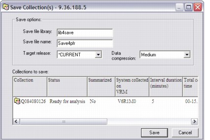
Figure A-9 Saving a collection
The Transfer to option now supports all collection types. It was modified as follows:
•PEX collections, PEX MGTCOL objects, CS collections, CS MGTCOL objects, DW collections, and Job Watcher collections all now support the transfer option.
•When sending data to IBM, the IBMSDDUU tool is now used.
•When you transfer multiple collections, they are saved and sent using the same save file instead of different ones.
•Monitors (or multiple monitors) can now be transferred.
•Path / file names increased to 100 chars from 50.
•You have complete control to set the file name to whatever you want, but the recommended format is given.
•You now have an option in the action list to FTP the collections to ECuRep.
•Mixed case passwords, user names, and file names are now supported, which fixes problems when you send data to and from AIX.
•The QIDRGUI/FTPFILE command now supports a GET action instead of the default of PUT. This command allows an iDoctor i user to receive data from another system (such as NMON data from an AIX box).
In all components that support copying a collection, you can now specify the collection name in the target library. You can use this function to copy a collection to a new name in the same library.
Data Viewer
The Data Viewer toolbar has a toolbar that shows all the idle waits (include all buckets) for wait bucket jobs and larger grouping graphs in CSI and Job Watcher. This toolbar is a toggle button that you can use to see the idle waits and click again to see the interesting waits. Previously, the idle waits were not shown for job or higher groupings. Figure A-10 shows an example.
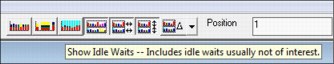
Figure A-10 Idle waits toggle button
There is a new menu, Choose Database Members, in the SQL editor that clears the current member selections and opens the member selection window.
In the record quick view, you can see the table alias name before the column name if it is known.
You can now click Save on the Data Viewer toolbar to save the current graph and legend as a JPG image.
You can click File → Create Shortcut to save a Data Viewer graph or table as a shortcut file (*.idr). The file can be sent to other users or saved on the PC to revisit the report later.
The interval grouping option on the Clock icon now has a five-minute and four-hour time interval specification.
The Data Viewer has a button, represented by the sum symbol, to run math over cells from the selected rows in a flyover as the user moves their mouse pointer over the data. The options are as follows:
•None (normal flyover behavior)
•Sum
•Average
•Minimum and Maximum
•Percent of, Delta (current - prior)
•Delta (prior - current)
There are also changes to the design of graphs and reports.
Side-by-side comparisons
You can use the side-by-side comparisons to sync up the scrolling and Y-axis scaling of any two graphs (or tables) in a Data Viewer.
When two or more graphs or tables exist in a Data Viewer, the buttons are ready for use. See Figure A-11.
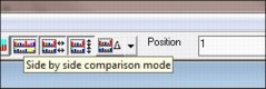
Figure A-11 Side by side comparisons
An example video of using side-by-side comparisons can be found at:
Table filtering options
Right-click the column that you want to filter. Set the wanted operator and value and click Apply to refresh immediately. See Figure A-12.
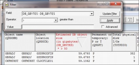
Figure A-12 Filter
More options are found by right-clicking a column:
•Sort
•Remove filter
•Hide column
•Unhide all columns
Graph filter options
You can use new graph filtering options to define a filter over the wanted column that is shown in the legend. Right-click the wanted column description and click Add Filter. See Figure A-13.

Figure A-13 Example of graph filter options
Collection Services Investigator
The folders available in the Collection Services Investigator (CSI) component changed. Instead of showing libraries that contain CS data, new folders are available, as shown in Figure A-14:
•Libraries containing CS database file collections (filterable)
•Historical summaries that contain broader periods of CS performance data
(weeks / months)
(weeks / months)
•CS objects for a list of all CS management collections objects on the system
The rest of the folders are described in “Main window” on page 868.
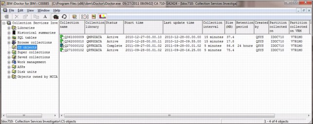
Figure A-14 Folders in the CSI component
Historical summaries
Historical summaries consist of consolidated or reduced sets of Collection Services data for graphing many days, weeks, or months of data at one time.
Figure A-15 gives an example of a Historical Summary Collection Overview Time Signature graph over 12 days of data.

Figure A-15 Historical Summaries - Collection Overview Time Signature
These data can be created in two possible ways:
1. Run the STRCSMON command (or use the Start Monitor menu option from the Historical Summaries folder), which summarizes new Collection Services data every day at a certain time and adds it to the system’s default Historical Summary repository.
2. Right-click one or more libraries and click Analyses → Run Historical Summary.
Use the one-hour grouping option when you create the Historical Summary.
Historical summaries provide a complete set of graphs similar to the graphs provided under normal collections. A full set of “average day” and “average week” graphs are also supplied. More information about historical summaries can be found at:
Capacity planning
You can now capture the selected collection's information and import it into the Workload Estimator. Use the Launch Workload Estimator menu on a collection, as shown in Figure A-16. A window opens with the average processor and disk statistics for the collection.
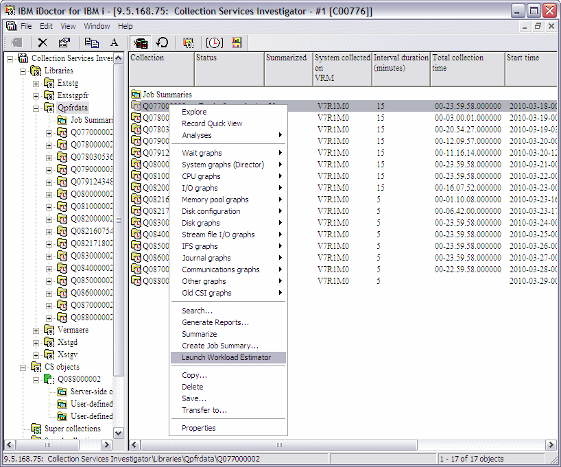
Figure A-16 Start the Workload Estimator
When you click Submit (Figure A-17), the data is sent to Workload Estimator for further analysis.
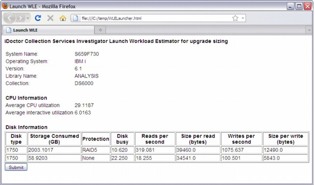
Figure A-17 Submit to WLE
Managing collections
On the same drop-down menu that is shown in Figure A-16 on page 877, you see that a Copy function was added. You can also use the Copy Performance Data (CPYPFRTA) command to obtain the same result. The Delete function now uses the Delete Performance Data (DLTPFRDTA) command.
The import data to WLE option is accessible from a CSI graph if a time range is selected. The numbers that are provided to WLE are based on the selected time period.
A search function, similar to the one in Job Watcher, is now available in this window. You can use it to generate a report that shows job records that are based on a specific job name, user, number, subsystem, pool ID, or current user profile. From these reports, you can drill down into the graphs for the wanted job over time. You can also search over multiple collections at one time by selecting the wanted collections in the CSI component view’s list side and then using the Search menu. After the search results are shown, you can drill down on the same set of collections that are provided for the wanted job or thread.
You can create graphs over multiple collections at one time in the same library. Select the wanted collections from the CSI component view's list side and then right-click and choose the graph of interest. Click Yes when prompted if the graph is to be created for all collections selected. From then on, any drill down that you do on rankings and the single object over time graphs apply to this same set of collections.
In CSI and PEX, you now have a Wait Buckets tab that shows the wait buckets or ENUM mapping. Right-click and select Collection → Properties → Wait Buckets, as shown in Figure A-18.
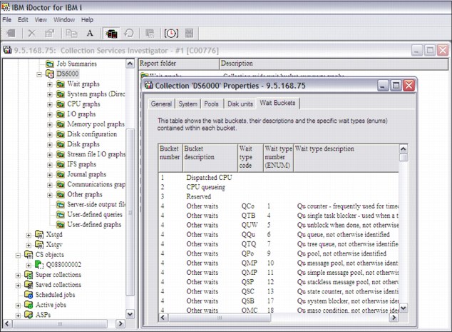
Figure A-18 Wait and ENUM display
Interval detail pages
The interval details property pages in CSI show key information for a thread/job and interval. These pages are like the ones in Job Watcher, and have a common 'general' section.
Situational analysis
To start a situational analysis, right-click the collection and click Analyses → Run Situational Analysis. You can also right-click the collection, click Analyses → Analyze Collection, and click Situations to configure the default situations to be used by CSI. See Figure A-19.
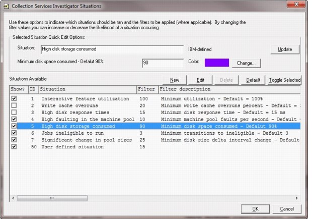
Figure A-19 Collection Services Investigator Situations
All the time interval-based Wait graphs include different background colors, each identifying a situation, as shown in Figure A-20.
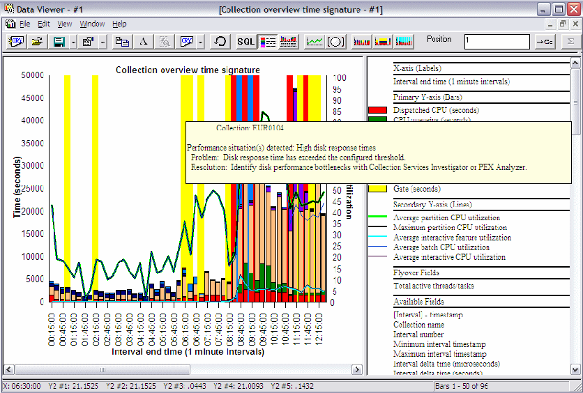
Figure A-20 Situational Analysis example
The current list of situations and the default minimum thresholds are shown in the following list:
•Interactive feature use high: 100%
•Write cache overruns: 20%
•High disk response times: 15 ms
•High faulting in the machine pool: 10 faults per second
•High disk storage consumed: 90%
•Jobs ineligible to run: Three instances for a job per interval
•Significant changes in pool size: 25% change from one interval to the next
External storage analysis
For an in-depth overview of this instrumentation, see 8.3.6, “External disk storage performance instrumentation” on page 405.
IASP Bandwidth analysis
The purpose of the IASP Bandwidth analysis is to analyze the Collection Services data with the intent to determine whether the system is a good candidate for migrating to Independent ASPs.
Right-click the collection and click Run IASP Bandwidth to kick off the analysis. When you run the analysis, you are prompted for several parameters:
•Compression rate: The estimated network (comm line) compression rate (between the system and the IASP). A value of 1 means no compression. 1.5 (the default) means 50% compression. Do not use values less than 1.
•Full system bandwidth: Estimated bandwidth that is required by system without IASPs (in megabits per second). Depending on the system or data, you might want to adjust this value to be much higher.
•IASP bandwidth: Estimated bandwidth that is required by system with IASPs implementation (in megabits per second). Depending on the system or data, you might want to adjust this value to be much higher.
•ASP filtering: You can use this option to select which ASPs to include when you run the analysis.
After you run the analysis, a new IASP bandwidth estimations folder is available that contains the generated table and a subfolder with graphs.
The IASP bandwidth estimate table represents the statistics that are generated by the analysis. The statistics that are generated include the number of blocks, writes, database write percentage, and various bandwidth estimates (all in megabits per second).
The IASP bandwidth overview graph displays the database writes for IASPs and the full system writes.
The IASP bandwidth overview graph with lag includes how much bandwidth lag there would be based on the parameter estimation values given when the analysis was created.
SSD candidate screening
Available at 7.1 or higher, SSD Candidate Screening helps determine whether SSDs might improve performance, as shown in Figure A-21. It uses data from QAPMDISKRB. It is similar to the SSD Analyzer tool.
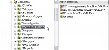
Figure A-21 SSD candidate screening
If you select SSD screening summary for ASP from the right pane, a graph opens in Data Viewer, as shown in Figure A-22.
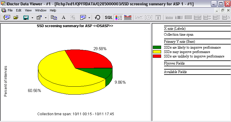
Figure A-22 SSD screening summary for ASP
Physical system graphs
You can now view what was collected by the IBM System Director tool for all partitions on which it was running, as shown in Figure A-23.
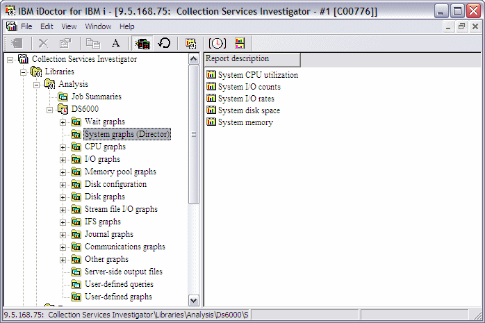
Figure A-23 Physical system statistics
These tools support all Power Systems as of V5R4.
•Processor use
•I/O counts
•I/O rates
•Disk space
•Memory
The information from the hypervisor for systems that are running release 6.1 or higher can now be viewed in the new System Graphs HMC folder (see Figure A-24).
The graphs shown vary depending on the data available. The QAPMLPARH file is required for the CPU graphs and in IBM i 7.1, the file QAPMSYSINT is required for the TLBIE graphs.
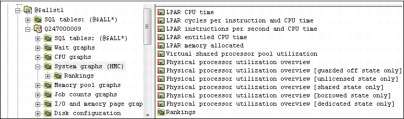
Figure A-24 System Graphs (HMC) folder
It includes the following graphs:
•LPAR CPU time: Shows the processor time that is used for all partitions (Figure A-25).
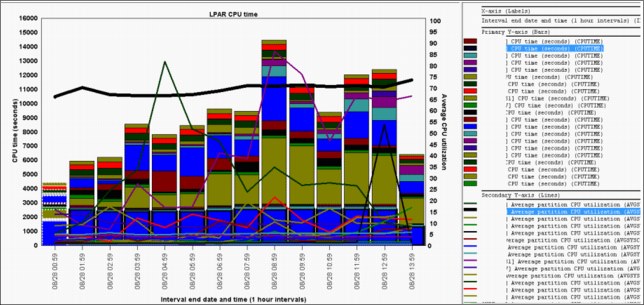
Figure A-25 LPAR CPU time overview graph
•LPAR cycles per instruction and CPU time: Same as previous but includes CPI on Y2.
•LPAR instructions per second and CPU time: Same as first graph but includes IPS on Y2.
•LPAR entitled CPU time: This graph breaks down the CPU time by entitled time versus uncapped time in excess of entitled capacity.
•LPAR memory allocated: Shows the memory consumption for all partitions (Figure A-26).
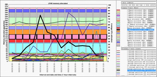
Figure A-26 LPAR memory allocated
•Virtual shared processor pool utilization.
•Physical processor utilization overview: Shows the average processor utilization for each physical processor over time (Figure A-27).
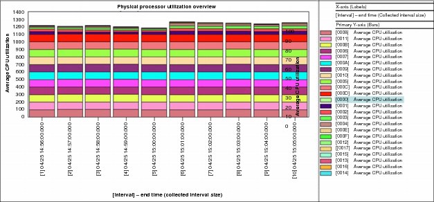
Figure A-27 Physical processor utilization overview
If the system is running IBM i 7.1 and file QAPMSYSINT exists, then a set of TLBIE graphs is shown (Figure A-28).
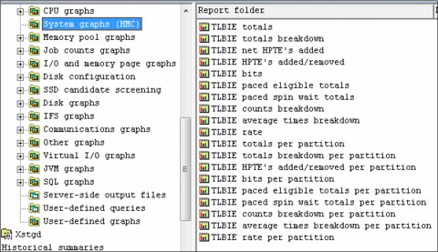
Figure A-28 System graphs (HMC), TLBIE graphs
An example of one of the TLBIE graphs is shown in Figure A-29.
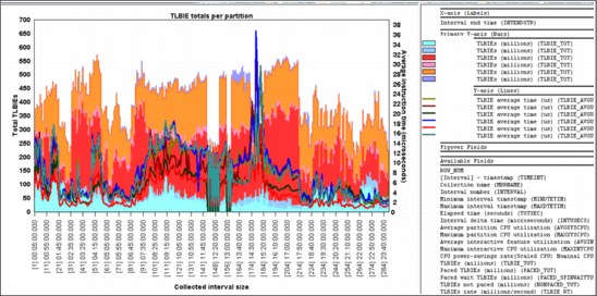
Figure A-29 TLBIE totals per partition
The Rankings folder contains the following graphs that rank the LPARs in various ways:
•LPAR CPU time
•LPAR cycles per instruction and CPU time
•LPAR instructions per second and CPU time
•LPAR advanced CPU time
•LPAR memory allocated
•LPAR donated processor time
•Physical processor utilization
•LPAR dedicated processor utilization
Shared memory graphs
If the QAPMSHRMP file is available, a shared memory graphs subfolder is available that contains the following additional graphs:
•Shared memory overview (Figure A-30)

Figure A-30 Shared memory overview
•Shared memory pool page faults (Figure A-31)
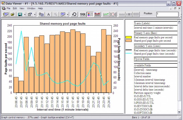
Figure A-31 Shared memory pool page faults
•Memory for I/Os overview (Figure A-32)
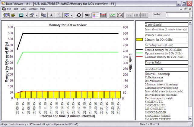
Figure A-32 Memory for I/Os
Disk graph updates
New types of graphs have been added that show a different color per ASP, disk type, disk group, or IOA type as shown in Figure A-33.
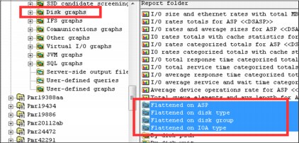
Figure A-33 Disk graphs, “flattened on” graph types
Job counts graphs
If you right-click a collection and select Collection → Job counts graphs, the following options are available:
•Job counts (Figure A-34)
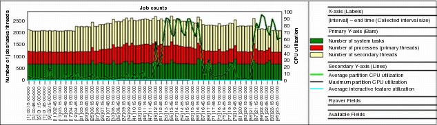
Figure A-34 Job counts
•Net jobs created
•Net jobs breakdown
•Job created / destroyed
•Job counts rankings (by job grouping) as shown in Figure A-35

Figure A-35 Job Counts by generic job name
•Net jobs breakdown rankings (by job grouping)
Memory pool graphs
If you right-click and select Collection → Memory pool graphs, you can generate graphs that contain the following information:
•Memory pool consumption (by percentage) (Figure A-36)
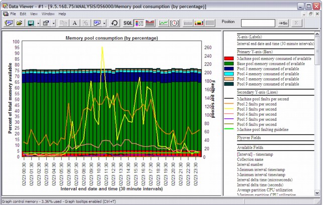
Figure A-36 Memory pool consumption
•Memory pool sizes (by percentage)
•Memory pool consumption
•Memory pool sizes
•Machine pool sizes and rates
•64K versus 4K page faults for pool <<JBPOOL>>
Additional graphs are also available under these folders:
•Flattened type (with pool filtering on drill down)
•Memory pool graphs (for pool sizes > 1 TB)
You can use the memory pool graphs to right-click the wanted pool and time range to drill down and see the jobs within the wanted pool in various ways.
There is also support to allow multiple collections to be graphed at the same time to compare the evolution in memory use. You can either select multiple collections and right-click and select the wanted memory pool graph, or use the Historical Summary analysis to graph multiple collections more easily.
Disk configuration reports
A new Disk configuration folder under the Collection menu contains information about the ASPs, IOPs, IOAs, and units on the system. This information includes information about the IOAs, including the read / write cache sizes. The first report provides a breakdown of disk capacity.
Two more reports show the same disk configuration data, where one is a flat table and the other is a tree. The tree provides counts and percentages of the units, IOAs, IOPS, and ASPs within each prior level grouping. To access these reports, right-click and select Collection → Disk configuration. The window that is shown in Figure A-37 opens.
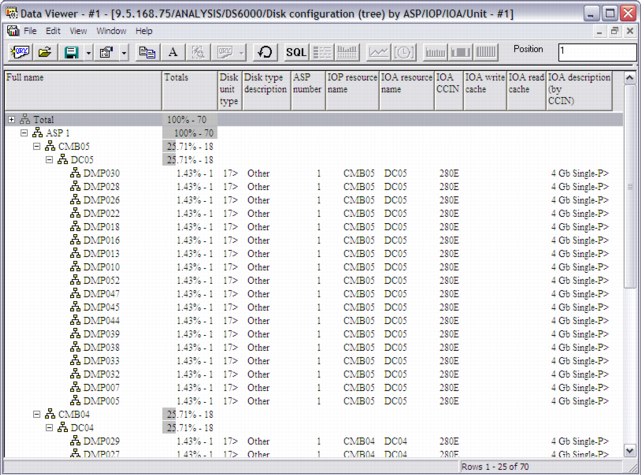
Figure A-37 Disk configuration by tree
A report called Capacity (in GBs) by ASP with paths is also provided.
Advanced disk graphs
As explained in “QAPMDISKRB” on page 306, there is a new structure for reporting the disk response times in a new set of buckets. These new statistics can be found by right-clicking and selecting Collection → Disk graph → Advanced. An example is shown in Figure A-38.
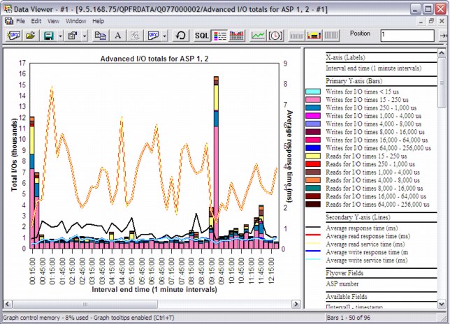
Figure A-38 Advanced disk graphs
12X loops and I/O hubs graphs
The 12x loops and I/O hubs folder (under the Communication graphs folder) contains three styles of graphs.
•Summarized: Summarizes the loop data over time.
– Summarized loops/hubs traffic
– Summarized 12x loops traffic
– Summarized I/O hub traffic
– Total traffic breakdown
– Send and receive traffic breakdown
– 12x loops traffic breakdown
– I/O hub traffic breakdown
•Rankings: Ranks each loop/port by throughput.
•Advanced: These graphs show every loop/hub (above the filter threshold) over time.
The seven summarized graphs provide drill downs into seven ranking graphs for the wanted time period.
Ethernet graphs
A new series of Ethernet graphs have been added under the Communication graphs folder as shown in Figure A-39.

Figure A-39 Ethernet LAN graph
J9 JVM graphs
A set of J9 JVM graphs at 6.1 and higher have been added. This includes overview graphs (all JVMs combined), rankings (by thread), and selected thread over time. The graphs included at each level are:
•J9 JVM heap sizes (includes allocated, heap in use, malloc, JIT, and internal sizes)
•J9 JVM allocated heap size
•J9 JVM heap in use size
•J9 JVM malloc memory size
•J9 JVM internal and JIT memory sizes
Enhanced graphs
Changes were applied to a number of graphing capabilities that support Version 6.1 and later:
•The communication graphs folder shows the following information:
– Average IOP uses
– Maximum IOP uses
– SSL authentications
•Under Disk graphs, new graphs named I/O size and Ethernet rates and Buffer overruns/underruns are now available.
•The collection overview wait graphs now show batch and interactive processor usage on the second Y axis.
•The wait bucket counts are added to the overview graphs for a single thread/job.
•The IP address family and formatted IP address is added to the end of the job search report.
•Flattened type graphs provide the capability to customize graph labels, hide values on the Y1/Y2 axis, change scaling, and use the graph definition interface to change the fields that are used, scaling, colors, and sizes.
Starting with Version 6.1, you now have the following information:
•A new graph for the selected job/user level called “Total pages allocated for <<OBJTYPE>> <<OBJDESC>>,” showing the total pages that were allocated and deallocated for the entire lifespan of the job.
•A new series of graphs under the I/O graphs folder shows the net pages that are allocated and net page frames that are requested. Net pages that are allocated are shown in megabytes and assume that the page size is 4 KB. Both sets of graphs include the usual rankings graphs to graph the data by thread, job, generic job, user, and so on.
Starting with Version 7.1, seizes and locks graphs were added over the 7.1 lock count fields in the QAPMJOBMI file. Run the Collection Summary analysis and then access the graphs by clicking Wait graphs and looking under the Seizes and locks folder.
Job Watcher
The folders available in the Job Watcher component changed. Instead of showing libraries that contain Job Watcher data, new folders are available, as shown in Figure A-40:
•Libraries containing Job Watcher database file collections (filterable).
•A definitions folder provides a list of Job Watcher definitions on the system.
•The rest of the folders are covered in 6.4, “IBM iDoctor for IBM i” on page 318.

Figure A-40 Job Watcher folders
Monitors
In the window to start a Job Watcher (or Disk Watcher) monitor, you can specify the maximum collection size (in megabytes) for each collection that is running in the monitor.
The next set of changes applies to the following monitor commands: STRJWMON, STRPAMON, and STRDWMON. These options can also be found in the GUI when you start a monitor.
The Collection Overlap (OVRLAP) parameter is no longer used. The monitor now detects that a new collection started before the previous one ended.
The Collection Duration (MAXSIZE) parameter can now be specified in minutes with a decimal point (for example, 59.5 minutes).
When you restart a monitor, if the Maximum Historical Collections (COLNS) parameter is reduced, there are added checks to delete the additional ones.
Deleting collections in a monitor is now done in a submitted job.
The following changes apply only to STRJWMON:
•Added a Resubmit Collections (RESUBMIT) parameter to submit new collections if a collection fails to start or quits early.
•Added a Max Consecutive Resubmits (MAXTRIES) parameter to indicate the number of times collections are resubmitted if the RESUBMIT parameter is set to *YES and the current collection ended prematurely.
Create Job Summary analysis
Right-click and select Collection → Analysis → Create Job Summary to produce job totals for the wanted jobs that are based on any filters, as shown in Figure A-41.
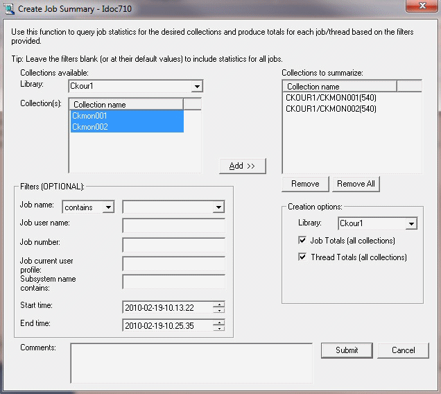
Figure A-41 Create Job Summary analysis
Collection Summary analysis
A collection is summarized by right-clicking and selecting Collection → Analyses → Analyze Collection (for full options) or by clicking Collection → Run Collection Summary. This new analysis is greatly simplified and many options that were previously on the Summarize Collection window were removed.
The Analyze Collection(s) window now has a new Situations button, which you can use to customize which situational analysis option to run, and the limits that are used for the situations (Figure A-42). The selected analysis can now run as a batch job. You can use a check box on the Analyze Collection(s) window to indicate whether this analysis is done instead of running it in the Remote SQL statement status view (a separate GUI QZDASOINIT job). The same analysis and similar options are found in the CSI component.
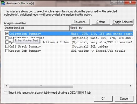
Figure A-42 Analyze Collection(s) window
There are advantages to running in batch:
•You can run start many analyses simultaneously.
•You can start the analysis, end your GUI session, and it keeps running.
•You can start multiple analyses on multiple systems without waiting on the remote SQL statement status view to run them in order.
Within the list of collections, the status field indicates which files are not yet created.
Situational analysis
This option can be found by clicking Collection → Wait graphs. It has new situations:
•Concurrent write not enabled
•Journal caching that are not properly used
•Jobs ineligible to run
•Long sync write response times
•Fixed allocated length setting on a varchar or lob type column is defaulted to 0 or is set too small
•Contention on DB in use table possibly because of a high number of opens and closes
•High number of creates and deletes by multiple jobs where all of the objects are owned by the same user profile
•Potentially large number of locks
•Deadlock because of DB record locks
Top threads and tasks graphs
These graphs can be found by clicking Collection → Wait graphs → Top threads over time. It displays the threads or tasks that spent the most time in the wanted wait bucket (such as processor) over time.
Objects waited on tab
The Objects waited on tab within the Interval Summary interface now includes the list of jobs that are waiting on an object but did not use processing time in the interval. Previously, only jobs that used processing time in the interval were shown. There is also a check box to show segments that are waited on.
Single interval rankings identifying flags
In Job Watcher, if you drill down into a wait bucket rankings graph on a single (job/thread) interval, you see the new flags field at the end of the job/thread name that contains the following possible values and meanings:
•W: Has a wait object.
•H: Holder.
•B: The current wait bucket is the same as current sort /filter bucket.
•S: Has an SQL client job (applies to 6.1 and higher only).
A wait object, holder, and a SQL client job are added to the flyover (if one exists).
SQL server mode job information
For Job Watcher 6.1 (with PTFs) or 7.1 only, the interval details property page now includes the SQL server mode client job if found, with the option to drill down and graph the job. See Figure A-43.
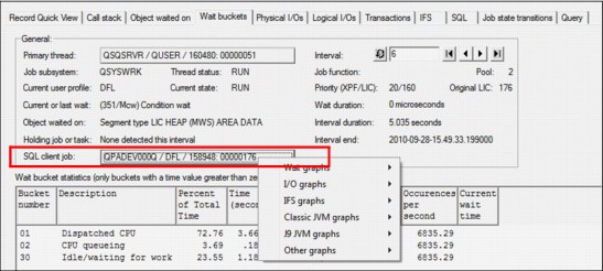
Figure A-43 SQL client job drill-down options on the Interval Details - Wait Buckets window
Status views
The Remote SQL Statement Status view was updated with new options:
•Remove/Cancel Selected cancels or removes running SQL statements.
•Copy Selected SQL Statement(s) to Clipboard.
•Add SQL Statement defines more statements to run in the view.
The Remote Command Status view was updated with new options:
•Remove/Cancel Selected cancels or removes running commands.
•Copy Selected Commands to Clipboard.
•Add Command defines more commands to run in the view.
Additional reporting options
There are several new reporting options for situational analysis, similar to the call stack reports based on the selected situation. From these options, you can double-click a job or thread to get into the call stack or run further drill down.
You can find JVM statistics on the Java virtual machine interval details tab and J9 call stacks on the Call Stack tab. The J9 Java entries are embedded within the regular Job Watcher call stacks. J9 Java call stack entries are not usable with the call stack reports.
You find a Situations tab in the Collection Properties (Figure A-44), showing all situation types known to Job Watcher and how many occurred in the collection.
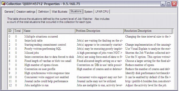
Figure A-44 Collection situations
In the Interval Details interface, a button was added to go to the primary thread from a secondary thread.
A new Call Stack Summary analysis was added to identify the call stacks, waits, and objects that are associated with the most frequently occurring call stacks that are found in the collection.
Reports were added under the Detail reports menu that show the top programs causing DB opens for the selected time period in a graph. The Detail reports - Call stack summary menu now has the following options:
•50 level call stacks,
•50 level call stacks with wait objects only
•50 level call stacks CPU current state only
Disk Watcher
The folders available in the Disk Watcher (DW) component changed. Instead of showing libraries that contain Disk Watcher data, new folders are available, as shown in Figure A-45:
•Libraries containing DW database file collections (filterable).
•A definitions folder that provides a list of DW definitions on the system.
•The rest of the folders are covered in “Main window” on page 868.

Figure A-45 Disk Watcher
Collections
In the Start Disk Watcher Wizard (Figure A-46), you now can collect the hardware resource file, schedule the collections, and check whether there are any PTFs. You can use another parameter in this window to set the maximum collection size (in MB) for each collection.

Figure A-46 Start a Disk Watcher monitor
A copy function for Disk Watcher collections was added. The CPYPFRCOL command (included with the OS) can also be used for this purpose.
The Change SQL Parameters interface now has options for changing the library and collection currently being used to display the graph.
Monitors
Disk Watcher monitor server commands were added. These commands are similar to the Job Watcher monitor commands and include STRDWMON, HLDDWMON, RLSDWMON, ENDDWMON, and DLTDWMON.
Support was added in the GUI to work with or start monitors in Disk Watcher for either Job Watcher or Disk Watcher. The same Monitors folder is also available in Job Watcher, which you can use to work with Disk Watcher monitors from the Job Watcher component.
Definitions
New iDoctor supplied Disk Watcher definitions are available.
•QFULLO
•QFULL1MINO
•QTRCO
•QTRC1MINO
The reload IBM-supplied definitions option must be used on systems that have definitions so that the new definitions are visible.
Reporting
The graph titles match the naming convention that is used by the trace graphs. The word pool was changed to disk pool, and disk unit to disk path.
A new trace Disk Watcher menu shows the top 25 I/Os rates. The graphs in Disk Watcher trace mode include the following (Figure A-47) information:
•I/O counts categorized totals
•I/O counts categorized writes
•I/O counts categorized reads
•I/O time categorized totals
•I/O time categorized writes
•I/O time categorized reads
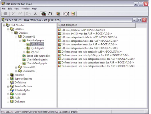
Figure A-47 Statistical graphs - By disk unit
Figure A-48 shows an example of these charts.
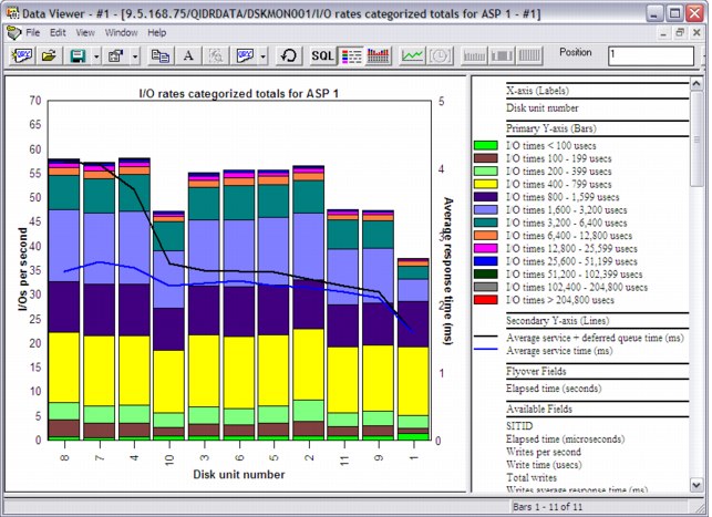
Figure A-48 Categorized I/O totals
PEX Analyzer
The folders available in the PEX Analyzer component were changed. Instead of showing libraries that contain PEX Analyzer data, new folders are available, as shown in Figure A-49 on page 904:
•Libraries: This folder displays libraries that contain PEX collections or libraries where active PEX collections created with the STRPACOL command (or the Start Collection Wizard) are running.
•Active collections: You can use this folder to work with any active PEX sessions on the system. This function is similar to the ENDPEX command that lists the active PEX sessions.
•PEX objects: You can use this folder to work with the PEX *MGTCOL objects on the system.
•Definitions: You can use this folder to work with PEX definitions.
•Filters: You can use this folder to work with PEX filters.
The rest of the folders are covered in “Main window” on page 868.
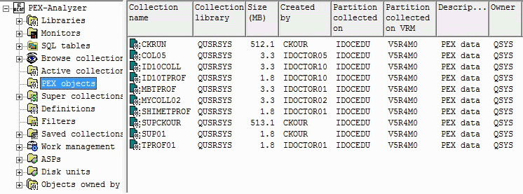
Figure A-49 PEX Analyzer
Definitions
The Add PEX Definition Wizard supports defining statistics counters into buckets 5 - 8.
The PEX Analyzer Add/Change PEX Definition interface supports the latest event additions and removals at 6.1/7.1:
•Program events that are removed as of 6.1+: *MIPRECALL, *MIPOSTCALL, *JVAPRECALL, and *JVAPOSTCALL
•Base event *CPUSWT added as of 6.1+
•Base events that are added as of 7.1: *PRCFLDSUSPEND, *PRCFLDRESUME, LPARSUSPEND, and *LPARRESUME
•Storage event *CHGSEGATR added as of 7.1
•OS *ARMTRC event added as of 6.1
•Sync event *MTXCLEANUP added as of 6.1
Because collecting DASD start events is no longer necessary for PDIO analysis, the Start PEX Analyzer Collection (STRPACOL) command now makes sure that the *PDIO_TIME event type always collects the *READEND, *WRTEND, *RMTWRTSTR, and
*RMTWRTEND events.
*RMTWRTEND events.
The STRPACOL command (and the Start Collection Wizard) now includes Format 2 events for all MI user problem types (*DB_OPEN, *DB_LDIO, and so on) and the Netsize problem type. Not collecting with Format 2 now requires you to create your own PEX definition.
In PEX Analyzer in the Start Collection Wizard, and when you use one of the iDoctor problem types, the default event format value for PMCO and Taskswitch is now Format 2.
When you create a collection, a QSTATSOPEN problem type collects DB opens into statistics counter #1. It runs concurrently with the QSTATSOPEN filter to ensure that only the user application program opens are counted. You can use this function to determine which programs or procedures caused the most opens by looking at the inline counter 01. The QSTATSOPEN problem type is a PEX definition that is created using ADDPEXDFN by the GUI before STRPACOL is run.
You can divide a large PEX collection into a more manageable size by using the Split option.
Monitors
PEX monitors can be started for systems that are licensed to both Job Watcher and PEX Analyzer. On the server side, there is a new set of commands for PEX monitors in the library QIDRWCH: STRPAMON, ENDPAMON, HLDPAMON, RLSPAMON, and DLTPAMON.
The Start iDoctor Monitor Wizard supports the creation of PEX monitors into *MGTCOL objects. There is an ENDPEX option, on the basic options window of the wizard, with three possible values: Create DB files, Create *MGTCOL, and Suspend.
Analyses
Several changes were implemented in this menu.
Classic analyses and support for the green panel QIDRPA/G* analysis commands was removed and replaced by the SQL-based analyses (SQL stored procedures).
The Analyses menu, found by right-clicking a collection, contains a list of all available analyses (Figure A-50). The menu also contains the Analyze Collection option, which allows a user to kick off several analyses at once.

Figure A-50 Analyses menu for a PEX collection
The Trace details analysis is available for any PEX collection that contains trace events and produces a SMTRMOD-like file. It handles retrieving and formatting event information from many of the PEX files including QAYPETIDX, QAYPEASM, QAYPESAR, QAYPEDASD, QAYPEPGFLT, QAYPETASKI, QAYPETSKSW, QAYPEPROCI, QAYPESEGI QAYPEMBRKT.
The Call stacks analysis displays the most commonly occurring call stacks for each event type collected. This analysis includes options to show the top programs causing opens and closes. Options are also available to view the call stacks by job and event type.
The TPROF analysis now has the tree table views that display the percentage of processor hits in various ways.
The TPROF analysis folder contains more reports to support MCLI analysis if format 4 PMCO events were collected.
A PDIO analysis is available and provides many graphs and drill downs for analyzing disk performance, including SSD performance. ASP prompting and comparisons are supported when you open a graph that contains data from more than one ASP.
PEX Analyzer has a new analysis called Hot Sectors. This SQL-based analysis is only available if the PDIO analysis was run. It allows disk activity to be measured by portions of the disk address of the I/O in megabyte chunks of either 1, 16, 256, or 4096.
A Data Area analysis is available for collections that collected data area events. It provides an SQL-based report similar to the SMTRDTAA file. A similar analysis for data queue events is available.
A CPU Profile by Job analysis is available if PMCO events were collected. It shows the estimated processor consumption during the collection over time and processor thread rankings for the wanted time periods.
The MI user event analyses (LDIO and data area) now resolve the user program if Format 2 events were collected. These analyses allow for MI entry / exit events to be excluded.
A database opens analysis, similar to the database LDIO analysis, provides statistics about the user program that is associated with the DB open events and reports 16 call level stacks, if DBOPEN FMT2 events are collected.
The new IFS analysis is equivalent to the classic version, except it also provides user program names for either MI entry / exit or FMT 2 call stacks, depending on what is available.
There is a new Netsize analysis for 6.1 and higher PEX Analyzer, including several new graphs with drill downs.
A save / restore analysis runs save / restore event parsing in the QAYPEMIUSR table into several reports.
In the Taskswitch analysis, added graphs show what the wait bucket time signature looks like for the wanted thread / task (also known as TDE). See Figure A-51. More drill downs and reporting options are also provided.
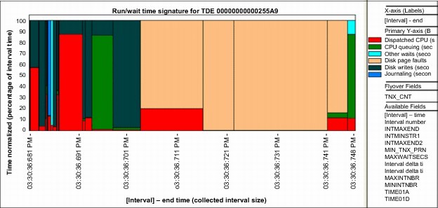
Figure A-51 Taskswitch run / wait time signature graph for a single job / thread / task (or TDE)
Reports
The Summarized CPU and I/O by job /pgm / MI instruction report contains two new fields:
•Inline CPU percent of job-thread total
•Inline elapsed time percent of job-thread total
The Summarized CPU and I/O by pgm / MI instruction report contains the inline processor percent of total and the inline elapsed time percent of total information.
Plan Cache Analyzer
Plan Cache Analyzer collects and analyzes snapshots of the system's SQL Plan Cache. It complements the features that are available in System i Navigator for analyzing the Plan Cache by providing several graphs and drill-down options that are not available there.
The plan cache is a repository that contains the access plans for queries that were optimized by SQE.
Starting Plan Cache Analyzer
Plan Cache Analyzer is included with a Job Watcher license and is a component of the IBM iDoctor for i suite of tools. iDoctor can be started by clicking Start → Programs → IBM iDoctor for IBM i. After the IBM iDoctor for IBM i application opens, you can start the Plan Cache Analyzer component from the Connection List View by double-clicking the correct system.
A list of available components appears in the next window. Double-click the Plan Cache Analyzer component or select Plan Cache Analyzer and click Launch to continue, as shown in Figure A-52.
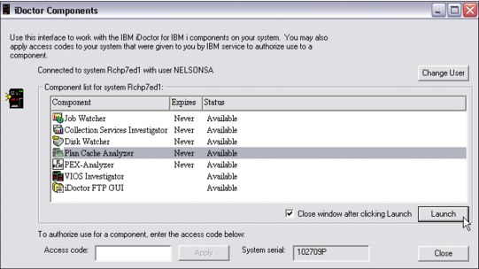
Figure A-52 iDoctor Components window
|
Plan Cache Analyzer: Plan Cache Analyzer is a subcomponent of Job Watcher and is only available if Job Watcher is installed correctly and a valid access code for Job Watcher is applied. This component is included with the Job Watcher license.
|
For more information about how to use Plan Cache Analyzer, see the IBM iDoctor for IBM i documentation at:
VIOS Investigator
VIOS Investigator combines NMON data and a VIOS to IBM i disk mapping process to help analyze the performance of your VIOS using the power of the DB2 database on IBM i.
You can use VIOS Investigator to import one or more NMON files into the tool. The NMON CSV files are converted and expanded into DB2 SQL tables, which are used to produce graphs with several drill-down options.
|
Graphing Options:
•Disk graphs (% busy, counts, sizes, rates, block sizes, service times, and response times)
•System configuration
•System graphs (Processor, memory, kernel, paging statistics, and processes)
•Processor graphs (Processor usage)
•TOP graphs (Processor usage, paging size, character IO, memory usage, and faults for the top processes)
|
If a valid disk mapping was created, then you can use the disk graphs to rank the data by disk name, disk unit, disk path, ASP, or disk type. Without the disk mapping, only rankings by disk name can be performed.
VIOS Investigator can also be used to analyze AIX and Linux systems using NMON data, but the focus is primarily on VIOS analysis with an emphasis on usage by IBM i customers.
VIOS Investigator is a no additional cost tool that is offered as-is and does not require an access code. To download VIOS Investigator, you must first accept the license agreement.
NMON
The VIOS Investigator data is created by the NMON or Topas_NMON command that is found in AIX.
On AIX V6.1 TL02 and Virtual I/O Server (VIOS) V2.1 (or higher), NMON is installed by default with AIX and the Topas_NMON command should be used for collecting data for use with
VIOS Investigator.
VIOS Investigator.
NMON is the primary/preferred collection tool of AIX performance statistics. NMON is similar in nature to Collection Services on IBM i. Both tools use time intervals and collect high-level statistics for processor usage, disk, memory and much more.
NMON data is collected into CSV (comma-separated values) files, and Collection Services uses DB2 tables. CSV files are difficult to analyze, especially if you want to analyze many of them. VIOS Investigator simplifies this issue by allowing users to import and then analyze multiple NMON files at once.
Disk mappings
Disk mappings (also known as correlations) refer to the VIOS to IBM i correlations between hDisks and IBM i disk unit numbers and disk path names that are assigned to them.
For comparison purposes with the Collection Services Investigator, whenever possible, the disk graphs in VIOS Investigator use the same colors, labels, and field names as the disk graphs in Collection Services Investigator. However, the number of disk metrics that are provided by NMON are far fewer than those disk metrics found in Collection Services (see the QAPMDISK file.)
In most cases, especially if there are any known hardware/system changes, collect the disk mapping before or immediately after you collect the NMON data on your VIOS. This action provides more graphing options (for example, rankings by unit, path, ASP, or disk type) that are otherwise not available.
Disk mappings are collected by using a program that is written on the IBM i that interrogates the HMC to acquire disk information that is useful when you perform the analysis that otherwise would not be available with just the NMON data.
Starting VIOS Investigator
VIOS Investigator is a component of the IBM iDoctor for IBM i suite of tools. iDoctor can be started by clicking Start → Programs → IBM iDoctor for IBM i. After the IBM iDoctor for IBM i application opens, the VIOS Investigator component is started from the Connection List View by double-clicking the system.
A list of available components appear in the next window. Double-click the VIOS Investigator component or select VIOS Investigator and click the Launch button to continue, as shown in Figure A-53.
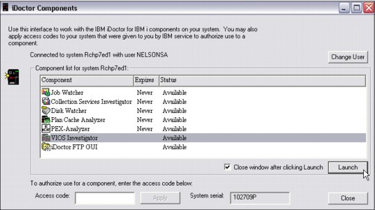
Figure A-53 iDoctor Components window
For more information about how to use VIOS Investigator, see the IBM iDoctor for IBM i documentation at:
iDoctor FTP GUI
A no additional cost GUI exists that provides FTP access to IBM i or other types of FTP servers. This GUI was created primarily for use with VIOS Investigator to ease the sending and receiving of performance data (such as NMON) to and from AIX (or VIOS) systems. It was tested only with connections to IBM i, AIX, or VIOS systems.
|
FTP connections: The FTP connections are provided through the Windows WININET APIs, which do not support any options for FTP using SSL or other secure FTP modes.
|
The FTP GUI is similar to other iDoctor components and can be accessed through the My Connections view. From the My Connections view, you can access this option by right-clicking the correct system and selecting Start FTP session from the menu, as shown in Figure A-54.

Figure A-54 Start FTP Session
You can also access the option from the Connection List View by double-clicking the system.
A list of available components appears in the next window. Double-click the iDoctor FTP GUI component or select iDoctor FTP GUI and click Launch to continue, as shown in Figure A-55.
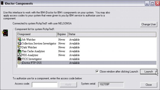
Figure A-55 iDoctor Components window
The FTP GUI window opens, as shown in Figure A-56.

Figure A-56 iDoctor FTP GUI window
|
IBM i system: If you connect to an IBM i system, you see subfolders to work with (either the Integrated File System (IFS) or the Libraries on the system). These options are not present for other types of connections.
|
There are several options available to you when you right-click a file or folder from the FTP GUI, including Upload, Download to PC, and Transfer to another system.
For more information about how to use the iDoctor FTP GUI, see the IBM iDoctor for IBM i documentation at:
MustGather Tools
The MustGather Tools GUI is an iDoctor GUI over library QMGTOOLS and the MG menu options provided on the green screen. The MustGather Tools were created by IBM Support to help automatically collect the many pieces of debug data critical to fixing complex problems more quickly.
More information about QMGTOOLs can be found on the following website:
HMC Walker
HMC Walker is a new option currently in beta test that uses the HMC lslparutil data to provide big picture views of performance across all LPARs attached to the HMC. If you want to join the beta test program contact:
HMC Walker provides views that display the configuration for the HMC and VIOS details. Several graphs are available with drill down into the LPARs using the appropriate iDoctor components (for VIOS, IBM i and AIX depending on the LPAR type.)
Figure A-57 shows the CPU used by several physical systems over 60 days.
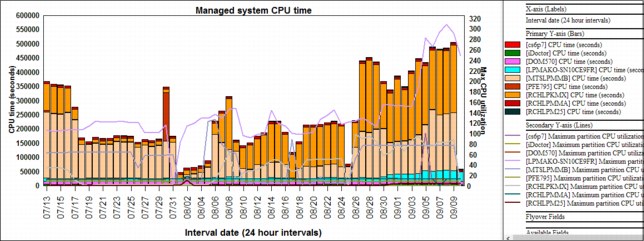
Figure A-57 Several physical systems over 60 days
Figure A-58 shows the CPU time for all LPARs across all of the physical systems. These LPARs are a mix of VIOS, AIX, and IBM i, and allow a user to pinpoint which LPARs are using the most CPU and drill down for further investigation.
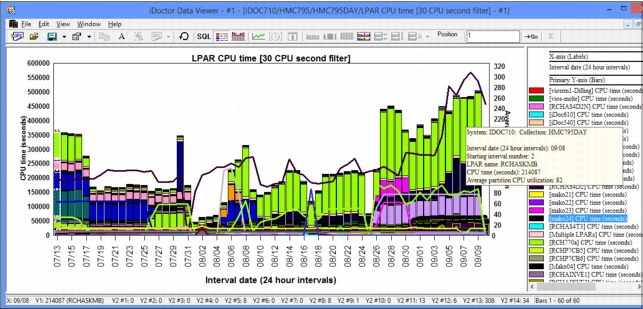
Figure A-58 CPU time for all LPARs across all of the physical systems
More information
For more information about the new features in iDoctor, go to:
You can also contact iDoctor team at: [email protected]
Presentations are created every few months with in-depth explanations of the latest features. You can find these presentations at:
Videos are available on the IBM iDoctor website at:
They can also be viewed directly on the YouTube Channel (20+ videos) for IBM iDoctor at:
..................Content has been hidden....................
You can't read the all page of ebook, please click here login for view all page.