
Chapter 14
Microsoft Office Excel 2003
This chapter provides a foundation to harness the power of spreadsheet program using Microsoft Office Excel 2003. It enables the user to effectively create worksheets quickly and efficiently. The reader will learn to create and format workbook using various in-built features of Excel. The chapter also covers various tools and features such as formulas and functions, inserting charts, and formatting cells. The chapter goes on to discuss insert formulas and graphics in a worksheet. The chapter concludes with an explanation on how to preview and print an Excel workbook.
After reading this chapter, you will be able to understand:
The basic concepts of spreadsheets using Microsoft Excel 2003
The steps required to create, open, save, and close a workbook
How to enter different types of data in a worksheet
How to edit the cell contents and the different ways to format a worksheet
The distinctive feature of Microsoft Excel—formulas and functions to dynamically perform mathematical operations from the data present in worksheets
How Excel converts data into different types of charts for graphical presentation to provide more visual clarity and impact
Different options of printing a workbook
14.1 INTRODUCTION
Microsoft Excel is a spreadsheet application that allows you to perform various calculations, estimations, and formulations with data. It is the electronic counterpart of a paper ledger sheet, which consists of a grid of columns (designated by letters) and rows (designated by numbers). Spreadsheets are popular because they represent a better alternative to manually computing mathematical calculations and are more accurate and time saving.
It also provides various facilities like inserting charts, creating graphs, analysing situations, and helps in decision-making. It is one of the best management tools. Excel provides flexibility to the user to manipulate the data without worrying about the size of the data for general applications. Excel 2003 permits a wide selection of options to be used in the creation of worksheets and allows you to create an impressive spreadsheet presentation.
14.2 STARTING MICROSOFT OFFICE EXCEL 2003
To open Microsoft Excel, perform any one of the following steps:
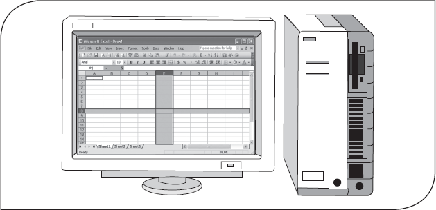
- Double-click the Microsoft Office Excel 2003 icon located on the desktop.
- Click start, point to All Programs, then point to Microsoft Office, and then select Microsoft Office Excel 2003 (Figure 14.1).
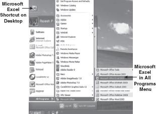
Figure 14.1 Starting Microsoft Excel
14.2.1 Microsoft Excel Environment
When Microsoft Excel is opened, the main screen of the application appears. This main window contains many parts; these parts are described below in detail (Figure 14.2).
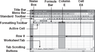
Figure 14.2 Main Microsoft Excel Window
Just like other office applications, Microsoft Excel has a title bar located at the top of the application window, which displays the name of the application and the active workbook. Below this bar is the menu bar, which contains different menus that have all the options, functions, and commands for the entire Microsoft Excel application. By default, Microsoft Office Excel 2003 contains nine menus, each of which has an associated pull-down menu. For example, the File menu contains commands to open, create, and print a workbook.
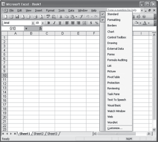
Generally, a toolbar is positioned just below the menu bar. Toolbar contains buttons, menus, or a combination of both that allows you to perform many tasks in a single-click. By default, Standard and Formatting toolbars are displayed in the Excel environment. Additional toolbars like Formula Auditing, and Chart toolbars can be added by right-clicking on the menu bar and selecting the desired toolbar(s) from the pop-up menu, as shown in Figure 14.3.
 w
w
Figure 14.3 Various Toolbars
Name Box and Formula Bar: Generally, the Name Box and Formula Bar are located below the toolbars. The Name Box displays the name of the active cell or selected range and can be used to name a range of cells. The drop-down menu next to the Name Box is used to locate previously named regions. The Formula Bar displays the contents of the selected cell in the worksheet. It includes text, numbers, formulae, and functions. You can also edit the contents of a cell from the formula bar.
Worksheet Tabs and Tab Scrolling Buttons: Worksheet tabs appear at the bottom of the Excel window. Each tab represents a single sheet. Worksheet tabs allow to move from one worksheet to another within the same workbook. The scrolling buttons that appear to the left of the worksheet tab allow you to scroll more quickly and easily through the sheets. You can rename a sheet by right-clicking on the worksheet and selecting Rename from the pop-up menu that appears.
Status Bar: The status bar is located at the bottom of the Excel window and displays information about a selected command or an operation in progress. When a command is selected, the left side of the status bar briefly describes the command. It also indicates operations in progress, such as opening or saving a file, copying cells, or recording a macro. The right side of the status bar shows whether keys such as CAPS LOCK, SCROLL LOCK, or NUM LOCK are turned on.
Worksheet and Workbook: Worksheet is the area on a spreadsheet in which you do all the work. A worksheet is made up of horizontal rows and vertical columns. An Excel worksheet contains 65,536 rows and 256 columns, and each intersection of a column and row forms a cell.
Individual worksheets are linked to form a workbook. Fundamentally, a workbook can be related to a very sophisticated ledger. It allows the user to work and store various kinds of related data within a single Excel file. By default, each workbook contains three worksheets (Sheet1, Sheet2, and Sheet3) that can be accessed by sheet tabs. If you need more than three worksheets, choose Worksheet from the Insert menu and to delete any worksheet, choose Delete Sheet from the Edit menu.
Columns, Rows, and Cells: In Microsoft Excel, the column is defined as the vertical space from top to the bottom of the window. There are 256 columns in a single worksheet which are labelled in alphabetical order (A, B, C…Z, AA, AB, AC…IV). The maximum number of characters, which can be inserted in a column, is 255. A row is defined as the horizontal space across the window. The rows are labelled in a numbered order (1, 2, 3, …, 65,536). The maximum limit of the height of a row is 409 points (547 pixels).
The basic unit in spreadsheet is a cell. A cell is formed by the intersection of a row and a column. This intersection gives the cell a unique address through which a cell can be referenced through its column name followed by its row number. For example, the intersection of row 2 and column B gives the cell B2. The cell that denotes the current position of the insertion point is known as active cell and has a dark border around it. Data written in a cell include text, decimal numbers, date and time, currency, percentage, and scientific notation.
14.3 WORKING WITH EXCEL WORKBOOK
In this section, you will learn the steps required to produce Excel workbook from scratch. This includes:
- Creating a new workbook
- Opening an existing workbook
- Saving a workbook and making a backup copy
- Closing the workbook and Excel application
14.3.1 Creating an Excel Workbook
Whenever you start Excel, it opens a new untitled spreadsheet window so that you can begin a new task. If Excel is already running and you want to create a new workbook, then click on New button (![]() ) on the Standard toolbar. A new workbook can also be opened by following the steps given below:
) on the Standard toolbar. A new workbook can also be opened by following the steps given below:
- Select New from the File menu to display the New Workbook task pane (see Figure 14.4).
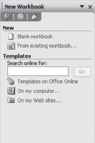
Figure 14.4 New Workbook Task Pane
- Now select Blank workbook under the New section. Excel by default opens a new workbook, which is sequentially numbered like Book1, Book2, and so on.
14.3.2 Opening an Existing Workbook
To open an existing workbook, follow any of the steps given below:
- Select Open from the File menu to display the Open dialog box (see Figure 14.5). You can also display the Open dialog box by clicking the Open button (
 ) on the Standard toolbar. The Open dialog box allows you to specify the name of the desired file in the File name drop-down box. If the desired file is not in the current location, you can locate it by navigating through Look in list box. Once the file is found, select the file and click the Open button.
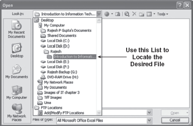
Figure 14.5 open Dialog Box
- Excel workbook can also be opened by double-clicking the Excel file icon, placed on the specified location.
14.3.3 Saving Workbook
Once a workbook is created, you can start typing the text, inserting graphics and charts, and so on. When this is done, you must save the workbook for future reference. To save the workbook, Microsoft Excel provides two menu options, namely, Save and Save As. If you are working on a untitled workbook, which has never been saved then using any of the option (Save and Save As) will have the same affect, it displays a Save As dialog box using which you can save the Excel file at the desired location (Figure 14.6).
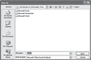
Figure 14.6 Save As Dialog Box
Once you have saved the new workbook, you can use the Save option to update changes made to a file. The Save As option is used to make multiple copies of the same file.
14.3.4 Closing a Workbook
After finishing all the work in the Excel spreadsheet, you may want to close the workbook. For this, follow any of the steps given below:
- Select Close from the File menu.
- Click at the Close Window button at the upper-right corner of the Excel window to close the current workbook. Note that there are two close buttons. One is located at the top of the application window, which closes the Excel application, while the second (lower) one present on the workbook closes only the current file (Figure 14.7).
Figure 14.7 Closing a Workbook
Note: If a user makes changes to a file and has not saved those changes, Excel will ask whether to save the changes before closing the file.
14.4 WORKING WITH WORKSHEET
In the previous section, we discussed how to create and save an Excel workbook. Now let us learn how to enter data in cells, select, and format cells. Apart from these activities, you will also learn how to insert and delete worksheets, copy and move data, and perform undo and redo operations.
14.4.1 Entering Data in Cells
In Excel, you can enter three types of data in a worksheet: labels (text), values (number), and formulae. Cells can also contain date and time. By default, labels are left aligned while values, time, and date are right aligned. Note that a label can include letters, spaces, punctuation, and numbers. Formulae are used to perform calculations on the values stored in a cell or range of cells. While using values, avoid commas and dollar signs as they are assigned special meaning in Excel (Figure 14.8).
Figure 14.8 Entering Data
To enter data into a cell, first select the cell and then type the data. As you type, notice that the data appear simultaneously in the Formula Bar and in the selected cell. The data is placed into the cell when you press the Enter key, the Tab key, or any of the Arrow keys. Data can also be entered in the Formula Bar, by selecting the cell and writing the data directly in the Formula Bar. If you enter more data than the cell can display, Excel will either truncate the display of the label or extend it over into the next cell. (In case of values, Excel displays a row of number signs #####.) This happens because the column is not wide enough to show the full content of the cell. To see the full content of the cell, follow any of the steps given below:
- Point the mouse pointer at the border of the cell (boundary line between two columns). When the pointer turns into a double-headed arrow, drag the width of the column to resize the cell.
- Double-click on the cell's right border to automatically adjust the column's width in order to best fit the contents (Figure 14.9).
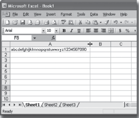
Figure 14.9 Resizing a Cell
14.4.2 Navigating through Cells
You can use either the mouse or the keyboard to navigate the Excel spreadsheet. To use the mouse, simply click in the desired cell. The keyboard offers a wider range of options for jumping to a particular location. The various shortcut keys used to move from one cell to another are listed in the Table 14.1.
Table 14.1 List of Keys Used for Moving in the Worksheet
| Keys | Description |
|---|---|
| Up Arrow Key | Moves one cell up |
| Down Arrow Key or Enter Key | Moves one cell down |
| Left Arrow Key | Moves one cell left |
| Right Arrow Key or Tab Key | Moves one cell right |
| Ctrl+Right Arrow Key | Goes to the end of the row |
| Ctrl+Left Arrow Key | Goes to the beginning of the row |
| Ctrl+Up Arrow Key | Goes to the top row of the sheet |
| Ctrl+Down Arrow Key | Goes to the bottom row of the sheet |
| Ctrl+Home | Goes to the top of the worksheet |
| Page Up | Moves active cell up one screen |
| Page Down | Moves active cell down one screen |
14.4.3 Naming of a Range of Cells
A range of cells is formed by selecting a group of adjacent cells in a worksheet. Naming a cell or a range of cells adds clarity and speeds up productivity especially when dealing with a very large spreadsheet. To name a range of cells, follow the steps given below:
- Select the cell or the range of cells.
- Click inside the Name Box to highlight the existing name of the cell.
- Type in the name for the selected cell or the range of cells and press the Enter key (Figure 14.10).
Figure 14.10 Naming a Range
14.4.4 Editing a Worksheet
While working with worksheets you need to edit the cell contents, add, or delete cells, rows, and columns, and so on. Excel provides a number of ways to format a spreadsheet. This includes changing fonts, colours, borders, etc.
Selecting Cells, Rows, and Columns: Whenever you want to make a change to a cell or a set of cells, you must first select it. To select an area, click on one cell, hold down the mouse button, and drag across the cells you want to include in the selection. Notice that as you move the cursor next to or onto a border, it changes from a white cross (![]() ) to an arrow-pointer. If you wish to select a large area of adjacent cells, use the Shift key to extend the selection. Click on the first cell of the range you want to select; then, while holding down the Shift key, click on the last cell in the range you want to select (Figure 14.11).
) to an arrow-pointer. If you wish to select a large area of adjacent cells, use the Shift key to extend the selection. Click on the first cell of the range you want to select; then, while holding down the Shift key, click on the last cell in the range you want to select (Figure 14.11).
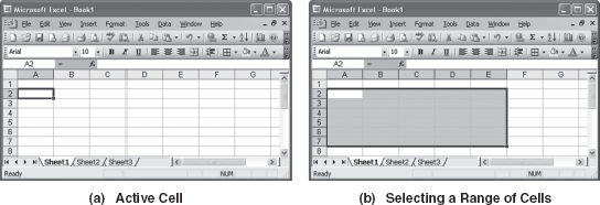
Figure 14.11 Selecting a Cell
An entire row or column can be selected by clicking on the desired row or column. For example, to select row “5” or the column “D,” click on the row heading or the column heading (see Figure 14.12).
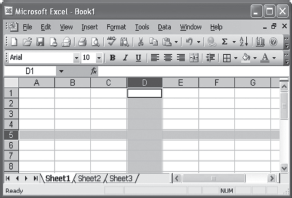
Figure 14.12 Selecting a Row and Column
Excel 2003 also allows for multiple selections and more than one range may be selected at the same time, that is, non-adjacent range of cells can also be selected. For this, select the first range of cells; then, while holding down the Ctrl key, select the second range of cells. If a user wants to select the entire worksheet, then this can be done by clicking on the grey square at the top-left of the spreadsheet (Figure 14.13).
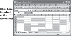
Figure 14.13 Selecting Non-Adjacent Range of Cells
Inserting Cells, Rows, and Columns: While working in Excel, users may be required to insert cells, rows, or columns to add new formulae or data. To insert cells, rows, or columns, select the cell and follow any of the steps given below:
- Select Cells from the Insert menu.
- Right-click on the cell and select Insert from the pop-up menu that appears.
When you perform any of the above-mentioned action, Microsoft Excel will display the Insert dialog box (see Figure 14.14).
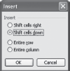
Figure 14.14 Insert Dialog Box
Choose any one option from the list and click OK. The various options present in this dialog box are listed in Table 14.2.
Table 14.2 Options of Insert Dialog Box
| Options | Description |
|---|---|
| Shift Cells Right | Moves the active cell to the right and inserts a cell in its place |
| Shift Cells Down | Moves the active cell down and inserts a cell in its place |
| Entire Row | Moves all cells of the row containing the active cell down and inserts a row |
| Entire Column | Moves all cells of the column containing the active cell right and inserts a column |
Deleting Cells, Rows, and Columns: Deletion removes the entire row or column from the spreadsheet. This action is similar to removing a Rows and Columns Inserting: Rows and columns can also be added by selecting Rows and Columns, respectively, from the Insert menu. The new row will be inserted above the row you have selected, and the new column will be inserted to the left of the selected column. The row numbers and column letters will change accordingly.
THINGS TO REMEMBER
Rows and Columns
Inserting: Rows and columns can also be added by selecting Rows and Columns, respectively, from the Insert menu. The new row will be inserted above the row you have selected, and the new column will be inserted to the left of the selected column. The row numbers and column letters will change accordingly.
Deleting: Multiple rows and columns can be deleted by first selecting one row or column and then holding down the Shift key and using arrow keys to select multiple rows and columns and then select Delete from the Edit menu or right-click on the cell and select Delete from the pop-up menu that appears.
Deleting Cells, Rows, and Columns: Deletion removes the entire row or a column from a Word table. To delete cells, rows, or columns, first select the cell and then follow any of the steps given below:
- Select Delete from the Edit menu.
- Right-click on the cell and select Delete from the pop-up menu that appears.
When you perform any of the above-mentioned action, Microsoft Excel will display the Delete dialog box (see Figure 14.15).
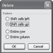
Figure 14.15 Delete Dialog Box
Choose from the list of options available and click OK. The various options present in this dialog box are listed in Table 14.3.
Table 14.3 Options of Delete Dialog Box
| Options | Description |
|---|---|
| Shift Cells Left | Deletes the active cell and moves all the remaining cells to the left |
| Shift Cells Up | Deletes the active cell and moves all the remaining cells up |
| Entire Row | Deletes the entire row containing the active cell |
| Entire Column | Deletes the entire column containing the active cell |
Editing Cell Contents: If you want to change the contents of the cell then, follow any of the steps given below:
- Single-click the cell to re-type the contents of the cell.
- Press F2 or double-click the cell to modify the contents of the cell.
- Use the arrow keys to select the cell and edit the contents of the cell.
- Select the cell to display the contents of the cell in the Formula Bar. Now, you can edit the contents of the cell directly in the Formula Bar.
When you perform any of the above-mentioned actions, press Enter key or click anywhere in the worksheet to accept the editing, or press Esc to cancel it.
Deleting Cell Contents: If you want to delete the contents of a cell, select the cell and follow any of the steps given below:
- Select Clear from the Edit menu and choose Contents option from the pop-up menu.
- Press Delete key.
Formatting Cells: Formatting data in Excel 2003 is similar to doing formatting in other Microsoft Office applications. Formatting is applied to the cells in order to change the appearance of the data stored in those cells. It is applied by altering the appearance of the cell by setting the alignment, typeface (font), size, style, and colour. Formatting can be done by using the Formatting toolbar or by using the Format Cells dialog box. To format the cell, follow the steps given below:
- Select the cell to be formatted.
- Use buttons on the Formatting toolbar to format the cell. Some of the buttons used in formatting cell are given in Table 14.4.
Table 14.4 Formatting Cell
| Command | Button | Description |
|---|---|---|
| Font | Changes the font of cell | |
| Font Size | Changes the size of the font | |
| Bold | Selected text appears in boldface | |
| Italic | Italicizes the selected text | |
| Underline | Underlines the selected text | |
| Align Left | Left aligns the paragraph or the selected text | |
| Center | Centre aligns the paragraph or the selected text | |
| Align Right | Right aligns the paragraph or the selected text | |
| Merge and Center | Merges and centres the contents of two or more cells | |
| Decrease Indent | Decreases the indent of the selected paragraph | |
| Increase Indent | Increases the indent of the selected paragraph | |
| Fill Color | Changes the colour of the cell | |
| Font Color | Changes the font colour of the selected text | |
| Currency Style | Applies currency style to the selected cell(s) | |
| Percent Style | Applies percent style to the selected cell(s) | |
| Comma Style | Applies comma style to the selected cell(s) | |
| Increase Decimal | Increases the number of digits after the decimal point | |
| Decrease Decimal | Decreases the number of digits after the decimal point | |
| Borders | Applies borders to the selected cell(s) |
Cells can also be formatted using the Format Cells dialog box. For this, follow the steps given below:
- Select the cell(s) to be formatted.
- Right-click on the cell and select Format Cells from the shortcut menu. This displays the Format Cells dialog box (see Figure 14.16).
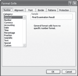
Figure 14.16 Format Cells Dialog Box
This dialog box contains a number of tabs to format the cell. These are Number, Alignment, Font, Border, Patterns, and Protection tabs. By default, this dialog box displays Number tab when opened.
Number tab Excel permits numbers to be formatted in many ways without changing the value of the number in a cell; number formats allow numbers to be represented so that they can be used in different kinds of scenarios. Different number formats are available under this tab. Some of the commonly used number formats are General, Number, Currency, Accounting, Percentage, and Fraction.
Alignment tab The options present in this tab allow you to change the position and alignment of the data within the cell. Data can be aligned with any or all four sides of a cell. Text can be aligned horizontally by selecting the various options such as Left (Indent), Center, Right (Indent), Fill, Justify, Center Across Selection, and Distributed (Indent). The selected cells can also be aligned vertically. This can be done by selecting the Top, Center, Bottom, Justify, or Distributed option in the Vertical dropdown box in the Alignment tab.
Note: The default alignment in Microsoft Excel 2003 aligns text to the left, numbers to the right, and centres logical and error values.
You can also change the orientation of text in a cell (from top to bottom, bottom to top, left to right, etc.). This can be done by entering either the exact amount of rotation required into the Degrees text box or drag the Text dial to give the desired level of rotation under the Orientation section.
Font tab The options present in this tab allow you to change font attributes such as font, size, style, etc. The Font tab can be used to set the font colour, underline text, and apply effects like, subscript, superscript, etc.
Border and patterns tabs The options present in border tab allow you to apply borders to the selected cells. There are different types of styles available to add border to selected cells. Click on the Outline button to add a basic border outside the selected cell range, or click on the Inside button to add borders between cells within the selected cell range. The options present in the Patterns tab allow you to apply shading to the selected cells.
Protection tab The options present in this tab allow you to lock the selected cell. However, it will have no effect unless the worksheet is protected. For this, select Protection from the Tools menu and choose Protect Sheet (Figure 14.17).
Figure 14.17 Formating cells
Using AutoFormat: Excel provides a feature known as AutoFormat that enables you to apply pre-defined layouts to the selected tables in the worksheet. These layouts do not alter the position of your data but apply colour backgrounds and rearrange borders with some attractive effects. To AutoFormat a table, select a range of the cells and follow the steps given below:
- Select AutoFormat from the Format menu to display the AutoFormat dialog box (Figure 14.18).
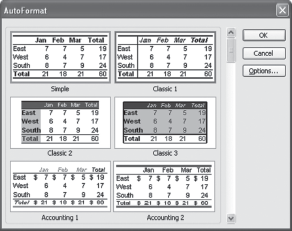
Figure 14.18 Using AutoFormat
- From this dialog box, choose the appropriate option and click OK to format the table accordingly (see Figure 14.19).
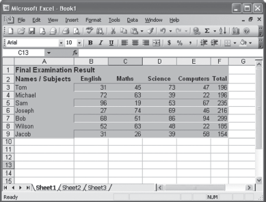
Figure 14.19 Cells After AutoFormat
If you want to revert to the original appearance of the cell, select Undo AutoFormat from the Edit menu.
14.4.5 Using Cut, Copy, and Paste in Excel
When you are working in a worksheet, you may decide to move the contents of one cell or a range of cells to some other part of the spreadsheet. If the text is to be moved within the same worksheet or to another worksheet, it should be first cut and then pasted. When you choose cut or copy, the cells are surrounded by a flashing dotted line, and their contents are not actually moved until you click in the cell where you want to paste. The contents of the selected cells do not disappear as they do in Word 2003. Copying the text is similar to the cut operation, except that copy retains the text at the original place but in case of cut, the text is removed from the original cell.
To perform the cut, copy, and paste operations, follow the steps given below:
- Select the cell or the range of cells to be moved or copied.
- In case you want to move the cell contents, choose Cut from the Edit menu or click the Cut button (
 ) on the Standard toolbar. If you want to copy the contents, choose Copy from the Edit menu or click the Copy button (
 ) on the Standard toolbar. Note that a dotted/fickering line surrounds the area that is cut or copied.
 - Click the mouse on the place in the workbook where you want to insert the text.
- Choose Paste from the Edit menu, or click the Paste button (
 ) on the Standard toolbar. The text that you copied to the clipboard is pasted to the location where the mouse is clicked (Figure 14.20).
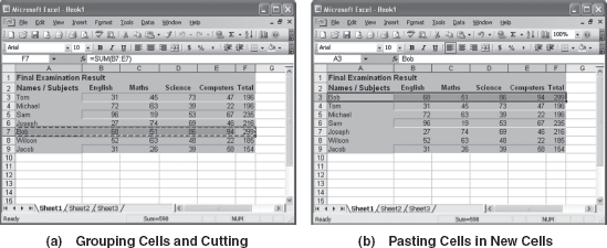
Copying Cells Using Fill Handle: In Excel, the Fill Handle provides an easy method of copying contents of the selected cells to the adjacent cells in a column or in a row. Fill handle appears on the worksheet when you move your mouse over the right bottom corner of the active cell. To copy a cell to the adjacent cells using the fill handle, follow the steps given below:
- Select the cell or range of cells to be copied.
- Point at the fill handle. The mouse pointer changes to black plus sign (
 ).
). - Drag the fill handle in the direction of the copy until the faded rectangle surrounds all the cells to be filled.
- Release the mouse button to copy the contents (Figure 14.21).
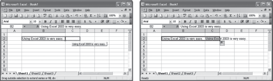
Figure 14.21 Using Fill Handle
THINGS TO REMEMBER
Linking Worksheets
In Excel, moving the information from a cell or a range of cells, rows, or columns is not just limited to a worksheet. Microsoft Excel 2003 gives the flexibility to link value from a cell in one worksheet to another. For example, the value of cell A1 in the worksheet1 and cell A2 in the worksheet2 can be added using the format “sheetname!celladdress.” The formula for this would be “=A2+[worksheet1.xls]sheet1!A1.”
Dragging Cells: Cell contents can also be moved to another cell by simply dragging the cell to point to the desired cell. To move a range of cells using drag and drop, follow the steps given below:
- Select the cell or the range of cells.
- Point at the border around the selection to change mouse pointer to a pointing arrow.
- Drag the border to the new location and release the mouse button (Figure 14.22).
Figure 14.22 Dragging cells
To drag the selected cells to a different sheet, hold down the Alt key and drag the selected area onto the sheet label. Excel will then display that sheet and you can position your selected cells as normal. Using this technique, you can restructure your spreadsheet at any stage in its development.
Sometimes, you may wish to create a list of numbers in cells. When the list of numbers is large say 1,000, then the process of entering the number manually becomes very time-consuming and exhausting. To automate this process, Microsoft Excel 2003 also allows you to fill series of data in an “intelligent” manner. For example, type any number in a cell, then type the next immediate number in the adjacent cell. To follow the same series pattern to a range of cell, select both cells and drag to the desired range using fill handle (Figure 14.23).
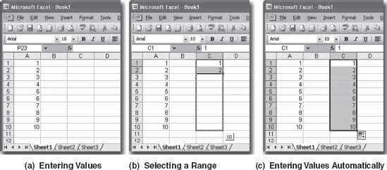
Figure 14.23 Inserting Series of Data
14.4.6 Finding and Replacing Cells
Find and replace option in Microsoft Excel is used to locate a particular word, phrase, or numeric value in a worksheet, or replace it with the new data. Microsoft Excel Find and Replace function swiftly and unerringly locates anything you are looking for, and once the desired text is located, it can automatically be replaced by the new data.
Data in Excel can be searched column- or row-wise in a worksheet. To find data within the worksheet, follow the steps given below:
- Select Find from the Edit menu, which opens the Find and Replace dialog box with Find as active tab (see Figure 14.24).
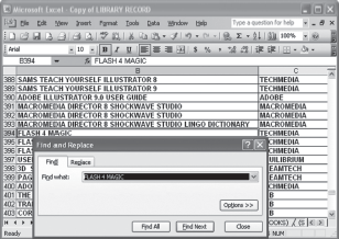
Figure 14.24 Find and Replace Dialog Box
- Type the data that you want to search in the Find what box and click Find Next button to find the first occurrence of the data.
- Keep on pressing the Find Next button until you are finished with finding data.
- To close the Find and Replace dialog box, click the Close button or press the Esc key.
To replace data within the worksheet, follow the steps given below:
- Select Replace from the Edit menu, which opens the Find and Replace dialog box with Replace as active tab (see Figure 14.25).
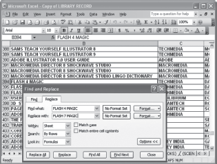
Figure 14.25 Find and Replace Dialog Box
- Type the data that you want to search in the Find what box.
- Click Find Next button to find the first occurrence of the data. If you want to replace the data then type the replacement data in the Replace with box.
- Select Replace button to replace each occurrence of the word individually. Keep on pressing the Find Next button until you are finished with finding and replacing the data.
- Click Replace All to replace all the occurrences of the data at once. Excel will display a message when it has replaced all the occurrences.
- To close the Find and Replace dialog box, click the Close button or press the Esc key.
14.4.7 Undo and Redo
Just like Word 2003, Excel remembers the actions performed on a file. If a portion of a worksheet is deleted or changed, you can revert to the original state by using the Undo command. This feature instructs the application to ignore the last action (whether it was deleting, copying, or moving). Note that Excel can undo or redo up to previous 16 actions (since last Save state) only as compared to Word, which allows user to undo or redo all actions until the document is closed (Figure 14.26).
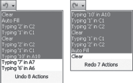
Figure 14.26 Undo and Redo Action
To undo the last action(s), click the Undo button (![]() ) on the Standard toolbar, or select Undo from the Edit menu. If you want to undo a number of actions at the same time then click the down arrow (
) on the Standard toolbar, or select Undo from the Edit menu. If you want to undo a number of actions at the same time then click the down arrow (![]() ) beside the Undo button to display a list of actions that can be undone.
) beside the Undo button to display a list of actions that can be undone.
If an undo action is set and you want to reverse it then Redo command can be used to reverse the undo action. To redo the last undo action, click on the Redo button (![]() ) on the Standard toolbar, or select Redo from the Edit menu. If you want to redo a number of actions at the same time then click the down arrow (
) on the Standard toolbar, or select Redo from the Edit menu. If you want to redo a number of actions at the same time then click the down arrow (![]() ) beside the Redo button to display a list of actions that can be redone.
) beside the Redo button to display a list of actions that can be redone.
14.5 FORMULAS AND FUNCTIONS
One of the distinguishing features of Excel is that it makes use of formulas and functions to dynamically calculate results from the data present in worksheets. Functions are routines built into the Excel spreadsheet while formulas are defined by the user and may include the built-in functions. Both Functions and formulas are widely used in simple as well as in advance computing. They provide the power to analyse data extensively.
Functions can be a more efficient way of performing mathematical operations than formulas. For example, if you want to add the values of cells C1 to C10, then using the formula you need to type “=C1+C2+C3+C4+C5+C6+C7+C8+C9+C10.” This can be tedious, a better, and a shorter way would be to use the SUM function and simply type “=SUM(C1:C10).”
14.5.1 Functions
Microsoft Excel contains many pre-defined or built-in formulas, which are known as functions. These can be used to perform simple or complex calculations. They perform calculations b using specific values, called arguments, in a particular order.
Parentheses are used to separate different parts of a formula. For example, in the formula =SUM(A1:A5), the parentheses separate the worksheet function from the cell references that the function is referring to. This is particularly important in longer or more complicated formulas, for example =((A2/4)+(A5-B3))*5. If a mistake is made and the parentheses in a formula do not match, an error message is displayed. Note that the parts of a formula contained inside the parenthesis are calculated first. Some examples of functions are =SUM(B4,G43,T70),=COS(A2), =AVERAGE(B1:B10).You can type functions in the Formula Bar directly into the cell or use the Function Wizard.
THINGS TO REMEMBER
Functions
Functions have three parts:
= sign, which tells Excel that a formula or function follows.
Function name, such as SUM for addition or AVERAGE for determining the average of a series of numbers.
Arguments on which the particular function operate. The argument contains cell references to let the function know which data to calculate. In Excel, a function can accept a maximum of 30 arguments. The argument must also be enclosed by parentheses.
To insert a function, follow the steps given below:
- Click the cell in which the function is to be entered.
- Select Function from Insert menu, or click Insert Function button (
 ) on the Formula Bar to display the Insert Function dialog box (Figure 14.27).
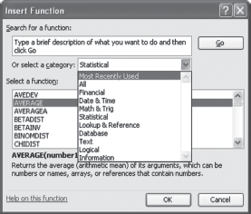
Figure 14.27 Insert Function Dialog Box
- Select a desired function category from the select a category drop-down box and choose the function name from the Select a function list which contains a list of available functions in the selected category. Once the desired function has been selected, click OK.
- After this, Excel displays a Function Arguments dialog box to help the user to create a function. In this dialog box, first click on the collapse button (labelled with a red arrow) to the right of the box labelled Number1 or Value1 (this depends on the function chosen) (Figure 14.28).
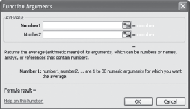
Figure 14.28 Function Arguments Dialog Box
- Drag the mouse to select the range of cells to be included as the first argument of the function and press Enter key.
- To specify additional arguments into the function, repeat Steps 4 and 5.
- Click OK to insert the function (Figure 14.29).
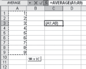
Figure 14.29 Inserting Function in Worksheet
Some of the categories of functions provided by Excel are:
- Math and Trig Functions
- Statistical Functions
- Date and Time Functions
- Logical Functions
- Text Functions
Math and Trig Functions: A user can perform simple calculations, such as rounding a number or calculating the total value for a range of cells with the help of mathematical and trigonometric functions. The various mathematical functions are listed in Table 14.5.
Table 14.5 Mathematical Functions
| Formula | Description | Example |
|---|---|---|
| SUM(number1, number2,…) | Adds all the numbers in a range of cells | SUM(10,20,30)
Output: 60 |
| ROUND(number, num_digits) | Rounds off a number to specified places of digits | ROUND(3.628, 2)
Output: 3.63 |
| SQRT(number) | Returns a positive square root of a given number. If the number is negative, SQRT returns the #NUM! error value | SQRT(25)
Output: 5 |
| ABS(number | Returns the absolute value of a number | ABS(-100)
Output: 100 |
| TRUNC(number, num_digits) | Truncates a number to an integer by removing the fractional part of the number | TRUNC(8.99,1)
Output: 8.9 |
Logical Functions: Excel has a number of functions that allow the user to evaluate values and make decisions based on the result of the evaluation. These functions are known as logical functions. The logical function returns either true or false value depending on the condition. The various logical functions used are listed in Table 14.6.
Table 14.6 Logical Fucntions
| Formula | Description | Example |
|---|---|---|
| AND(logical1, logical2, ...) | Returns value TRUE if all its arguments are true and returns FALSE if one or more arguments are false | AND(1+2=3, 2-2=0, AND(1+2=3, 2-2=1)
Output: False |
| NOT(logical) | Reverses the value of its argument | NOT(1+1=2)
Output: False NOT(1+1=1) Output: True |
| OR(logical1, logical2,...) | Returns TRUE, if any argument is TRUE and returns FALSE only when all arguments are FALSE | OR(1+2=3, 2-2=1)
Output: True OR(1+2=2, 2-2=1) Output: False |
Statistical Functions: In addition to mathematical functions, Excel provides a great deal of assistance to 0compute statistical data. All the functions are simple and take only a set of obser vations as arguments. The various statistical functions used are listed in Table 14.7.
Table 14.7 Statistical Functions
| Formula | Description | Example |
|---|---|---|
| MAX(number1, number2,...) | Returns the largest value in a given set of values | MAX(60,25,5)
Output: 60 |
| MIN(number1, number2,...) | Returns the smallest value in a given set of values | MIN(60,25,5)
Output: 5 |
| AVERAGE(number1, number2,...) | Calculates the arithmetic mean of all values in the list | AVERAGE(60,25,5)
Output: 30 |
Text Functions: In Excel, text functions are used not only to convert a value to text but also to join several text strings into one text string. Many functions are available that enable you to manipulate text strings, convert numeric entries into text strings, and convert numeric text entries into numbers. The various text functions used are listed below in Table 14.8.
Table 14.8 Text Functions
| Formula | Description | Example |
|---|---|---|
| CONCATENATE (text1, text2,...) | Joins several text strings into one text string | CONCATENATE (“GrandTotal”, “Total”) Output: Grand Total |
| LEN(text) | Returns the number of characters in a text string | LEN(“INDIA”)
Output: 5 |
| LOWER(text) | Converts all upper case letters in a text string to lower case | LOWER(“INDIA”)
Output: India |
| PROPER(text) | Capitalizes the first letter in each word of a text | PROPER(“INDIA”)
Output: India |
| UPPER(text) | Converts a text string to upper case | UPPER(“india”)
Output: INDIA |
| TRIM(text) | Removes all spaces from a text string except for single spaces between words | TRIM(“INDIA”)
Output: INDIA |
Date and Time Functions: The date and time functions are used for working with date and time. Excel uses serial numbers to store dates, giving each day of each year a unique number. The var ous date and time functions used are listed below in Table 14.9.
Table 14.9 Date and Time Functions
| Formula | Description | Example |
|---|---|---|
| DATE(year, month, day) | Returns the number that represents the date in Excel date-time code | DATE(1979,9,6)
Output: 9/06/79 |
| TIME(hour, minute, second) | Returns the number that represents a particular time | TIME(19,23,7)
Output:7:23 PM |
| NOW() | Returns the current date and time | NOW()
Output: 4/30/10 8:39 |
14.5.2 Using AutoSum
The SUM function is used more often than any other function. To make this function more accessible, Excel includes an AutoSum button on the Standard toolbar, which inserts the SUM function into a cell. It is a great tool to use when you want to quickly add the contents of a range of cells. To use AutoSum, follow the steps given below:
- Select the cell where you want the sum to appear.
- Click the AutoSum button (
 ) on the Standard toolbar. AutoSum inserts a formula that uses the SUM function. Clicking on the AutoSum, the cells get surrounded by a flashing dotted line. This dotted line is called a marquee. Excel puts this around the range of cells you want to add up and inserts the range reference in the formula.
 - If this is the correct range, then press the Enter key. If not, type or highlight the correct range and press the Enter key or Enter button (
 ) to apply the formula (Figure 14.30).
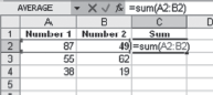
Figure 14.30 Using AutoSum
14.5.3 Formulas
Formulas are mathematical expressions built in Excel that instruct the computer to carry out calculations on specified sets of numbers in the rows and columns. A formula always begins with an equal sign (=) followed by some combination of numbers, text, cell references, and operators. If a formula is entered incorrectly, an ERROR IN FORMULA message will appear. If you forget to enter the initial (=) sign, Excel will treat the expression like a text string and the values will not be calculated. Note that Excel evaluates a formula in a specific order: from left to right following the order of operations.
Suppose, cell A1 contains 25 and cell A2 contains 90 and you want to add values in cell A1 and A2 in A3. For this, follow the steps given below:
- Select the cell where formula is to be inserted. In our case, the cell is A3.
- Type “=” followed by the operation (say, SUM) to be performed.
- Type the first and second cell names, separated by a colon (A1:A2).
- Press the Enter key or click the Enter button () on the Formula Bar. Now the formula appears in the Formula Bar while the cell (A3) contains the result of the formula as shown in Figure 14.31.
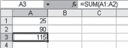
Figure 14.31 Using Formulas
Relative, Absolute, and Mixed Referencing: Referring to cells by their column and row labels (such as “A1”) is called relative referencing. When a formula contains relative referencing and it is copied from one cell to another, Excel does not create an exact copy of the formula. It will change cell addresses relative to the row and column they are moved to. For example, if a simple addition formula in cell C2 =SUM(A2:B2) (see Figure 14.32[a]) is copied to cell C3, the formula would change to =SUM(A3:B3) to reflect the new row. To prevent this change, cells must be called by absolute referencing, and this is accomplished by placing dollar signs “$” within the cell addresses in the formula.
Figure 14.32 Relatice, Absolute and Mixed Referencing
For example, if the formula in cell C2 would read =SUM($A$2:$B$2) (see Figure 14.32[b]) in which both the column and row of both cells are absolute, the formula will not change when copied. Mixed referencing can also be used where only the row or column is fixed. For example, in the formula =SUM(A$2:$B2) (see Figure 14.32[c]), the cell reference A$2 indicates relative column and absolute row and the cell reference $B2 indicates absolute column and relative row.
Editing and Deleting Formulas: A formula can be edited or deleted if required. To delete a formula, simply click on the cell that contains the formula and press the Delete key. If you want to alter the formula, follow the steps given below:
- Click the cell that contains the formula.
- Click in the Formula Bar, change the formula and press the Enter key.
Handling Operators in Formula: In Microsoft Excel 2003, operators specify the type of calculation that is to be performed on numbers or quantities. Excel includes four different types of calculation operators:
- Arithmetic Operator
- Text Operator
- Comparison Operator
- Reference Operator
All these operators have been listed in Table 14.10.
Table 14.10 Operators Used in Excel Formulas
| Operator | Meaning |
|---|---|
| * | Multiplication |
| / | Division |
| + | Addition |
| ‒ | Subtraction |
| % | Per cent |
| ^ | Exponentiation |
| = | Equal to |
| > | Greater than |
| < | Less than |
| >= | Greater than or equal to |
| <= | Less than or equal to |
| <> | Not equal to |
| & | Concatenates or combines two values to produce one continuous text value |
| : (colon) | Known as range operator. Produces one reference to all the cells between two references, including the two references, for example, D3:D7 |
| , (comma) | Known as union operator, which combines multiple references into one reference, for example, SUM(D3:D7, F15, B4) |
| (space) | Known as intersection operator, which produces on reference to cells common to the two references (A7:C7 B6:B8) |
Error Values: An error may occur in Excel while working with formulas when the intended task is not carried out in a proper way. For example, if you intend to add cells (A1: A4) and one of the cells, say A3, contains text, then the correct output will not be shown in the selected cell and an error state is said to have occurred. The errors may also occur due to some other reasons. Some of the common errors are listed in Table 14.11.
Table 14.11 Error Values
| Type of Error | Description |
|---|---|
| ###### | This is not exactly a kind of error; it just specifies that the result is too long to fit in the selected cell. This error can be corrected by making the column wider |
| #DIV/0! | This type of error occurs when a number is divided by zero. The error can be corrected by making sure that the divisor is not zero |
| #NAME? | This type of error occurs when there is a name in the formula that Excel cannot recognize. This error can be avoided by selecting a name from the Name Box instead of typing it. If you type a function, check the spelling and verify that the function exists or if users perform operations on text, enclose it in double quotation marks. |
| #REF! | This type of error occurs when cell reference is invalid. For example, when the user deletes cells referred to in a formula or cells are pasted and moved elsewhere. This error can be corrected by entering the formula again |
| #VALUE! | This type of error occurs when wrong operands or arguments are used within a formula. This error can be corrected by checking the passed arguments again and if wrong then passing them again |
14.6 INSERTING CHARTS
In Excel, numerical data can be easily converted into a chart for graphical presentation of the data. Charts provide more visual clarity than tables of data and, therefore, have more impact. Several types of chart are possible in Microsoft Excel, and each type has a number of variations. The chart types include pie charts, bar charts, line charts, etc. Whatever the type, all charts are linked to the worksheet data. This means that data values can be amended even after the chart has been created and the chart will automatically be updated.
Microsoft Excel allows a chart to be placed in two ways, as an embedded chart or a chart sheet. Embedded charts appear as objects on worksheets and can be resized and positioned to appear alongside tabular information or other charts and objects, whereas chart sheet exists as a separate sheet in a workbook. Chart sheets are, perhaps, a little easier to manipulate but when printed, they appear alone on the page. It is, therefore, possible to adjust the page orientation, headers, footers and other page attributes for the chart without affecting other worksheets.
Types of Chart: Excel allows you to create charts of different types. You can choose from the list of chart types available. Some of the commonly used chart types are:
- Area (
 ): This is used when a user wants to emphasize change over time.
 - Surface (
 ): In this chart, temperature and time are plotted together to show the tensile strength they produce.
 - Bar (
 ): This chart compares values with the different values given.
 - Radar (
 ): In this chart, each category of information has its own line radiating out from the centre.
 - Column (
 ): This chart is very similar to a bar chart, except that the bars are aligned vertically instead of horizontally.
 - Bubble (
 ): This chart shows three sets of variables, represented by the two axes and the size of the bubble.
 - Line (
 ): This chart is useful for comparing trends.
 - XY (Scatter) (
 ): This is useful for comparing a set of values with the average or predicted values.
 - Pie (
 ): This chart is used to compare a set of figures.
 - Doughnut (
 ): This chart is very similar to a pie chart, except that it can show more than one set of figures. Each ring of the doughnut represents a set of figures.
14.6.1 Creating Charts
One of the simplest and easiest methods to create a chart is by using the Chart Wizard. This wizard helps in creating a chart by displaying a series of dialog boxes. The dialog boxes included are selecting a chart type; selecting a format for the chart; specifying how the data are arranged; and adding a legend, axis titles, and a chart title. To insert a chart, follow the steps given below:
- Enter the data into the worksheet, which is to be converted into a chart as shown in Figure 14.33.
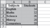
Figure 14.33 Worksheet Data
- Select Chart from the Insert menu or click the Chart Wizard button (
 ) on the standard toolbar to view the first Chart Wizard dialog box.
 - Choose the Chart type and Chart sub-type from the available list. Then click Next (Figure 14.34)
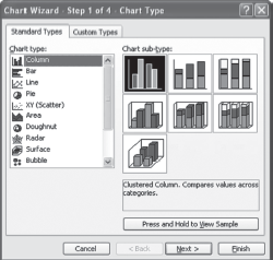
Figure 14.34 Chart Type Dialog Box
- Select the data range (if different from the area highlighted in step 1) and click Next (Figure 14.35).
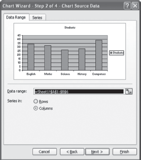
Figure 14.35 Chart Soource Data Dialog Box
- Now the Chart Options dialog box appears (see Figure 14.36). This dialog box allows you to enter the name of the chart and titles for the X- and Y-axes. By clicking on the tabs, one can change the axes, gridlines, legend, data labels, and data table. Click Next.
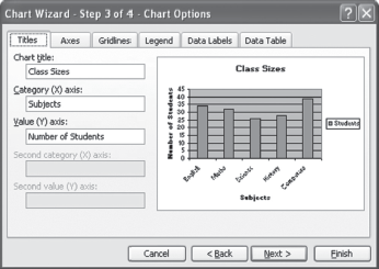
Figure 14.36 Chart Options Dialog Box
- The Chart location dialog box appears. This is the last step in Chart Wizard. This dialog box prompts you to specify the location of the chart. Click As new sheet if the chart is to be placed on a new, blank worksheet or select As object in to embed the chart in an existing worksheet as shown in Figure 14.37.
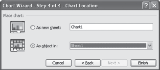
Figure 14.37 Chart Location Dialog Box
- Click Finish to create the chart. The chart appears on the screen as shown in Figure 14.38.
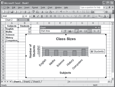
Figure 14.38 Chart on the Worksheet
Resizing and Moving Chart: Chart can be easily resized by clicking on the border of the chart. Doing this, the resizing handles appear on the border of the chart. Handles on the corners resize the chart proportionally while handles along the lines will stretch the chart.
A chart can be moved by selecting the chart, then holding down the left mouse button, and dragging the chart to a new location. Elements within the chart such as the title and labels can also be moved within the chart (Figure 14.39).
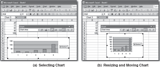
Figure 14.39 Resizing and Moving Chart
14.6.2 Using Chart Toolbar
Once a chart is inserted, it can be changed and enhanced by using the Chart toolbar. If the Chart toolbar does not appear, right-click anywhere on the menu bar and select Chart from the shortcut menu (Figure 14.40). The various buttons available on the Chart toolbar are listed in Table 14.12.
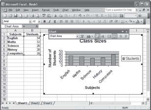
Figure 14.40 Selecting Chart for Editing
Table 14.12 List of All the Available Buttons on the Chart Toolbar
| Command | Button | Description |
|---|---|---|
| Chart Objects | Used to select different objects in a chart | |
| Format Chart Area | Used to edit the chart area | |
| Chart Type | Used to select a different type of chart | |
| Legend | Used to show or hide the chart legend | |
| Data Table | Displays the data table instead of the chart | |
| By Row | Displays the data by rows | |
| By Column | Displays the data by columns | |
| Angle Clockwise | Used to angle the text in the downward direction | |
| Angle Counterclockwise | Used to angle the text in the upward direction |
Changing the Chart Type: If a user after making a particular type of chart feels that the chosen type does not suit or meet the requirements, then a different type of chart can be chosen from the Chart toolbar to change the type of chart (Figure 14.41).
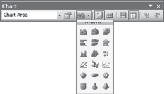
Figure 14.41 Different Chart Types
14.6.3 Saving a Chart
You can save charts for easy reference in future, thus reducing the time involved in making the same chart repeatedly. To save a chart, follow the steps given below:
- Select the chart and choose Chart Type from the Chart menu to display the Chart Type dialog box.
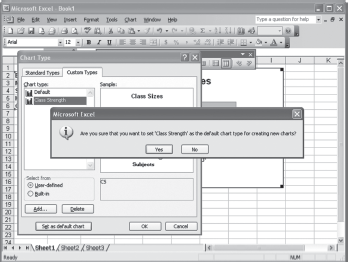
- In the Custom Types tab, choose User-defined and click Add. This displays the Add Custom Chart Type dialog box.
- Type a name for the graph in the Name text box and the description for the graph in Description box (if required) and click OK to close the Add Custom Chart Type dialog box (Figure 14.42).
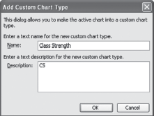
Figure 14.42 Setting a Default Chart
- Click Set as default chart button, a message box for confirming the action appears. Click Yes to set the selected chart as the default chart.
- Click OK to save the chart (Figure 14.43).
14.7 SORTING
Excel allows you to sort the data in any order. To perform this, follow the steps given below:
- Click in the column by which you want to sort the data or select a specific range in a column that is to be sorted.
- Select Sort from Data menu to display the Sort dialog box (Figure 14.44).
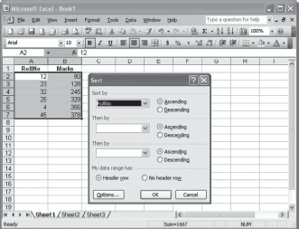
Figure 14.44 Sort Dialog Box
- By default, Excel sorts all the data in ascending order. If you want to sort in descending order, select Descending. Note that you can sort the data up to three fields at a time.
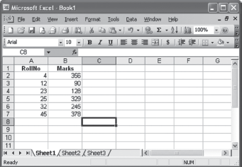
- Click OK to sort data and close the Sort dialog box (Figure 14.45).
14.8 PRINTING IN EXCEL
Printing in Microsoft Excel is similar to printing in other Windows-based applications. However, several options, particularly those concerned with arranging the page, are specific to the application.
14.8.1 Setting Page Layout
Page Layout option is used to view the existing page layout or to set a new layout. To set a new layout, select Page Setup from the File menu to display the Page Setup dialog box. This dialog box has four tabs: Page, Margins, Header/Footer, and Sheet.
Page Tab: Click on the Page tab to make changes to the page layout. This tab allows a user to make changes to any of the following:
- Orientation: Select Portrait or Landscape in the Orientation section.
- Paper size: Display the Paper size drop-down box to select the required paper size.
- Scaling: This is used to reduce or enlarge the print.
- Print quality: Choose the quality needed. This depends upon the printer installed on the computer.
- Page numbering: To begin page numbering, select the First page number text box and enter the number that is needed (Figure 14.46).
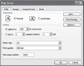
Figure 14.46 Page Setup Dialog Box
Margins Tab: Margins are the empty space between the text and the left, right, top, and bottom edges of a printed page. By default, margins are “1” inch at the top and bottom and “.75” inch from left and right. You can make changes to the top, bottom, left, and right margins of the document in order to create more space for the data present on the page or to add some extra space when binding a document (Figure 14.47).
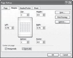
Figure 14.47 Setting Margins
Header/Footer Tab: Headers and footers can be easily created in Excel. There are some standard as well as customized options available for creating headers and footers. You can also create custom headers and footers by selecting Header/Footer tab in the Page Setup dialog box (see Figure 14.48).
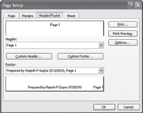
Figure 14.48 Adding Headers and Footers
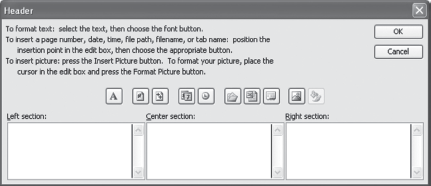
To create header (or footer), click on the down arrow to the right of the Header (or Footer) list box to display a list of available headers (or footers). Click on the appropriate header (or footer) needed. If you want to create a different header (or footer), then click on the Custom Header (or Custom Footer) button to display the Header (or Footer) dialog box (Figure 14.49). In the Left section box, enter any data that are needed to be present at the left margin of the header (or footer). In the Center section box, enter the data that are required at the centre of the header (or footer). Similarly, in the Right section box, enter the data required at the right margin of the header (or footer). You can also add date and time to header (or footer) using the Date and Time icons, respectively. When finished, click OK to close the dialog box. The new header (or footer) will be displayed in the Page Setup dialog box in the Header (or Footer) list box.
Sheet Tab: You can change the print range and elements to be printed such as headings, gridlines, and comments, and also the order of pages to be printed in this tab. This tab allows a user to specify any of the following:
- Columns or Rows to Repeat: Click on the icon to the right of the Rows to repeat at top text box in the Print titles area and drag over the rows that the user wants to repeat at the top of the page. Click on the icon in the right of the Columns to repeat at left text box and drag over the columns that are to be repeated at the left of the page.
- Elements That will Print: Select the elements to print, that is, Gridlines, Comments, Draft Quality, Black and White, and Row and Column Headings.
- Order of Pages to Print: Select Down, then over, or Over, then down.
- Print Range: In the Print area text box, enter the worksheet range to be printed (Figure 14.50)
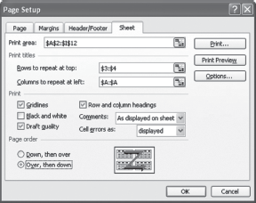
Figure 14.50 Sheet Tab
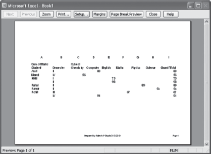
14.8.2 Print Preview
Print preview is a way to view the printed worksheet on-screen before printing the final output. Previewing the worksheet is a good way to identify formatting errors, such as incorrect margins, overlapped text, boldfaced text, and other text enhancements. This helps in saving costly printer paper, ink, and time. To view a worksheet in print preview mode, choose Print Preview from the File menu or click the Print Preview button (![]() ) on the Standard toolbar. Note that the options available in print preview mode in Excel are similar to Word. Click Close to return to the worksheet or Print to continue printing (Figure 14.51).
) on the Standard toolbar. Note that the options available in print preview mode in Excel are similar to Word. Click Close to return to the worksheet or Print to continue printing (Figure 14.51).
14.8.3 Printing Worksheets
Once you have completed formatting and editing worksheet(s), you can print the whole sheet (Active sheet), part of the sheet (selection), or several sheets (workbook). To print, click the Print button (![]() ) on the Standard toolbar, or select Print from the File menu to display the Print dialog box. This dialog box allows you to select the number of copies and how many pages of the document you want to print. It also contains Print what section where a user can choose the printing area. Some of the options provided under this section are:
) on the Standard toolbar, or select Print from the File menu to display the Print dialog box. This dialog box allows you to select the number of copies and how many pages of the document you want to print. It also contains Print what section where a user can choose the printing area. Some of the options provided under this section are:
- Selection: Choose this option if only a selected part of the worksheet is to be printed.
- Entire workbook: Choose this option if the entire workbook is to be printed.
- Active sheet: Choose this option if the Active worksheet (active sheet is the sheet where user is working) is to be printed.
After selecting the appropriate option, click OK to print (Figure 14.52).
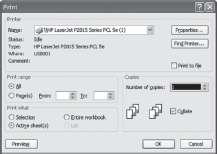
Figure 14.52 Print Dialog Box
Important Keyboard Shortcuts
Document Actions
| Action | Shortcut Key |
|---|---|
| Open a Workbook | CTRL+O |
| Create a New Workbook | CTRL+N |
| Close a Workbook | CTRL+F4 |
| Close a Workbook | CTRL+F4 |
| Save As | F12 |
| Save | CTRL+S |
| Help | F1 |
| CTRL+P | |
| Close Excel Application | ALT+F4 |
Text-Formatting Actions
| Action | Shortcut Key |
|---|---|
| Bold | CTRL+B |
| Italics | CTRL+I |
| Underline | CTRL+U |
| Edit Active Cell | F2 |
| Format Cells Dialog Box | CTRL+1 |
Selecting Cells
| Action | Shortcut Key |
|---|---|
| Entire Column | CTRL+Spacebar |
| Entire Row | SHIFT+Spacebar |
| Cells Left of Active Cell | SHIFT+Left Arrow |
| Cells Right of Active Cell | SHIFT+Right Arrow |
| Entire Worksheet | CTRL+A |
Text-Editing Actions
| Action | Shortcut key |
|---|---|
| Undo and Redo | CTRL+Z, CTRL+Y |
| Cut | CTRL+X |
| Copy | CTRL+C |
| Paste | CTRL+V |
| Find | CTRL+F |
| Replace | CTRL+H |
| Go To | CTRL+G |
| Action | Shortcut key |
|---|---|
| Move to Start of Row | Home |
| Move to Start of Column | CTRL+Left Arrow |
| Move to Next Worksheet | CTRL+Page Down |
| Apply AutoSum | ALT+= |
| Current Date | CTRL+; |
| Current Time | CTRL+: |
| Spelling | F7 |
Let Us Summarize
- Microsoft Excel is a spreadsheet program that allows you to perform various calculations, estimations, and formulations with data. It is the electronic counterpart of a paper ledger sheet, which consists of grid of columns and rows.
- To open Microsoft Excel, click Start, point to All Programs, then point to Microsoft Office, and then select Microsoft Office Excel 2003.
- To create a new workbook, click on New button (
 ) on the Standard toolbar. Alternatively, select New from the File menu.
 - To open an existing workbook, click on the Open button () on the Standard toolbar. Alternatively, select Open from the File menu.
- To save the workbook, Microsoft Excel provides two menu options, namely Save and Save As.
- To close the workbook, select Close from the File menu.
- To find and replace text within the worksheet use the Find and Replace dialog box, which can be displayed by selecting Find and Replace from the Edit menu.
- To undo the last action, select Undo from the Edit menu. To redo the last undo action, select Redo from the Edit menu. You can also use the Undo button (
 ) and Redo button (
 ) from the Standard toolbar.
 - In Excel, numerical data can be easily converted into a chart for graphical presentation of the data. Charts provide more visual clarity than tables of data and, therefore, have more impact.
- One of the simplest and easiest methods to create a chart is by using the Chart Wizard. This wizard helps in creating a chart by displaying a series of dialog boxes.
- Print preview is a way to view the printed workbook on-screen before printing the final output. To view a worksheet in the print preview mode, choose Print Preview from File menu or click the Print Preview button (
 ) on the Standard toolbar.
 - To print a worksheet, click the Print button (
 ) on the Standard toolbar. Alternatively, use the Print dialog box, which can be displayed by selecting Print from the File menu.
Exercises
Fill in the Blanks
- .................. are popular because they represent a better alternative to manually computing mathematical calculations and are more accurate and time saving.
- By default, .................. and .................. toolbars are displayed in the Excel environment.
- Microsoft Excel worksheet contains columns .................. rows and .................. columns.
- Press .................. or .................. the cell to modify the contents of the cell.
- The options present in .................. tab allow you to change the font attributes such as font face, size, style, and effects if desired by the user.
- The .................. provides an easy method of copying the contents of the selected cells to the adjacent cells in a column or in a row.
- .................. are mathematical expressions built in Excel that instruct the computer to carry out calculations on specified sets of numbers in the rows and columns.
- .................. reverses the value of its argument.
- .................. chart shows three sets of variables, represented by the two axes and the size of the bubble.
- A user can also create custom headers and footers by selecting .................. tab in the Page Setup dialog box.
Multiple-choice Questions
- Which of these is not a font style?
- Bold
- Underline
- Italic
- Footer
- A cell range is represented as follows:
- (A6.A8)
- (A6–A8)
- (A6:A8)
- (A6,A8)
- .................. appear at the bottom of the Excel window.
- Sheet tabs
- Name Box
- Formula bar
- Title bar
- Workbook is a collection of ..................
- Page Setup
- Buttons
- Worksheets
- Charts
- Borders tab in Format Cell dialog box is used to apply ..................
- Borders
- Shading
- Background colours
- All of these
- Excel provides a feature known as .................. that enables you to apply pre-defined layouts to selected tables in the worksheet.
- AutoFormat
- Header and Footers
- Undo and Redo
- None of these
- .................. and .................. option in Microsoft Excel is used to locate a particular word, phrase, or numeric values in a worksheet, or replace it with something else.
- Undo, Redo
- Formulas, Functions
- Find, replace
- None of these
- One of the distinguishing features of Excel is that it makes use of .................. to dynamically calculate results from the data present in worksheets.
- Formulas and functions
- Goto
- Tables
- All of these
- Microsoft Excel contains many pre-defined or built-in formulas, which are known as ..................
- Formatting Cells
- Functions
- Relative Referencing
- AutoSum
- An error may occur in MS Excel while working with .................. when the intended task is not carried out in a proper way.
- Formulas
- Tables
- Headers and Footers
- None of these
State True or False
- The Name Box displays the name of the active cell or selected range and can be used to name a range of cells.
- The intersection of row 12 and column E gives cell 12E.
- In Excel, the rows are labelled in a numbered order (1, 2, 3, ..., 65536).
- The Save option is used to make the multiple copies of the same file.
- To select a large area of adjacent cells, the Ctrl key is used to extend the selection.
- The cell contents can also be moved to another cell by simply dragging the cell to point to the desired cell.
- Excel allows the users to create mathematical formulas and execute functions.
- In the Bar chart, each category of information has its own line radiating out from the centre.
- Data entries are categorized into three basic types: labels, values, and formulas.
- By default, Excel sorts all the data in descending order.
Descriptive Questions
- Describe the steps involved in creating a chart.
- Show the steps involved in naming a range of cells.
- Explain Number, Font, and Alignment tab in Format Cell dialog box.
- Explain Find and Replace in Excel 2003.
- What is the difference between Formulas and Functions? Show the steps involved in inserting Functions.
- Explain the AutoSum feature with the help of an example.
- Describe the various types of error values that might occur while working with Functions and Formulas.
- What are the various types of charts available in Excel 2003?
- Explain the various options available on the Charts toolbar.
- Explain the Margin tab, Sheet tab, and Header/Footer tab in the Page Setup dialog box.
ANSWERS
Fill in the Blanks
- Spreadsheets
- Standard, Formatting
- 65,536, 256
- F2, double-click
- Font
- Fill handle
- Formulas
- NOT(logical)
- Bubble
- Header/Footer
Multiple-choice Questions
- (d)
- (c)
- (a)
- (c)
- (a)
- (a)
- (c)
- (a)
- (b)
- (a)
State True or False
- True
- False
- True
- False
- False
- True
- True
- False
- True
- False