
Mobile Robots
General Concepts
This chapter presents the fundamental general concepts of mobile robots that can move from one place to another autonomously within a predefined workspace to achieve their desired goals. Specifically, the chapter (i) provides a list of the main historical landmarks of general robotics and mobile robots, (ii) discusses the locomotion issues of ground (wheeled, legged) mobile robots, (iii) investigates the wheel and drive types of mobile robots (nonholonomic, omnidirectional) and, (iv) introduces the concepts of mobile robot degree of mobility, degree of steerability, and maneuverability.
Keywords
Wheeled mobile robot; maneuverability; fixed wheel; castor wheel; universal wheel; mecanum wheel; differential drive; bicycle drive; tricycle drive; omnidirectional drive; Ackerman steering; skid steering
1.1 Introduction
Mobile robots are robots that can move from one place to another autonomously, that is, without assistance from external human operators. Unlike the majority of industrial robots that can move only in a specific workspace, mobile robots have the special feature of moving around freely within a predefined workspace to achieve their desired goals. This mobility capability makes them suitable for a large repertory of applications in structured and unstructured environments. Ground mobile robots are distinguished in wheeled mobile robots (WMRs) and legged mobile robots (LMRs) Mobile robots also include unmanned aerial vehicles (UAVs), and autonomous underwater vehicles (AUVs). WMRs are very popular because they are appropriate for typical applications with relatively low mechanical complexity and energy consumption. Legged robots are suitable for tasks in nonstandard environments, stairs, heaps of rubble, etc. Typically, systems with two, three, four, or six legs are of general interest but many other possibilities also exist. Single-leg robots find rare applications because they can only move by hopping. Mobile robots also include mobile manipulators (wheeled or legged robots equipped with one or more light manipulators to perform various tasks).
The objective of this chapter is to present the fundamental general concepts of WMRs. In particular, the chapter
• provides a list of the main historical landmarks of general robotics and mobile robots;
• discusses the locomotion issues of ground (wheeled, legged) mobile robots;
• investigates the wheel and drive types of mobile robots (nonholonomic, omnidirectional); and
• introduces the concepts of mobile robot degree of mobility, degree of steerability, and maneuverability.
1.2 Definition and History of Robots
1.2.1 What Is a Robot?
The term “robot” (robota) was used for the first time in 1921 by the Czech writer Karel Capek and means slave servant or forced labor. In science and technology there is not a global or unique definition of a robot. When Joseph Engelberger, the father of modern robotics, was asked to define a robot he said: “I can’t define a robot but I know one when I see one.” The Robotics Institute of America (RIA) defines an industrial robot as “a reprogrammable multi-functional manipulator designed to move materials, parts, tools, or specialized devices through variable programmed motions for the performance of a variety of tasks which also acquire information from the environment and move intelligently in response.” This definition does not capture mobile robots.
The definition adopted in the European Standard EN775/1992 is as follows: “Manipulating industrial robot is an automatically controlled reprogrammable multi-purpose, manipulative machine with several degrees of freedom (DOF), which may be either fixed in place or mobile for use in industrial automation applications.
Ronald Arkin says: “An intelligent robot is a machine able to extract information from its environment and use knowledge about its work to move safely in a meaningful and purposive manner.”
Rodney Brooks says: “To me a robot is something that has some physical effect on the world, but it does it based on how it senses the world and how the world changes around it.”
In summary, a robot is referred in the literature as a machine that performs an intelligent connection between perception and action. An autonomous robot is programmed to work without human intervention, and with the aid of embodied artificial intelligence can perform and live within its environment. Today’s mobile robots can move around safely in cluttered surroundings, understand natural speech, recognize real objects, locate themselves, plan paths, and generally think by themselves. Intelligent mobile robot design employs the methodologies and technologies of intelligent, cognitive, and behavior-based control. Mobile robots must maximize flexibility of performance subject to minimal input dictionary and minimal computational complexity.
1.2.2 Robot History
The history of robots can be divided in two general periods [1,2]:
1.2.2.1 Ancient and Preindustrial Period
The first robot in the worldwide history (around 2500–3000 BC) is the Greek mythodological mechanical creature called Talos (“Τάλως”) [3]. This name is attributed both to a human being (the son of Daedalus’ sister Perdika) and a mechanical artificial entity constructed by Hephaestus, under the order of Zeus, with bronze body and a single vein from the neck up to the ankle, where a copper nail blocked it out. Talos was gifted by Zeus to Europe who afterward gave him to her son Minos to guard Crete. Talos died when the Argonaut Poas removed the copper nail from his heel. This resulted in the spilling out of the ichor (“the blood of the immortals”) flowing in the Poas’ vein. The name Talos was given to Asteroid 5786 discovered by Robert McNaught, on September 31, 1991 at Siding Spring Observatory in Coonabarabran, New South Wales (Australia). Around 350 BC the friend of Plato Archytas of Tarentum constructed a mechanical bird (“pigeon”) which was propelled by steam. This represents one of the earlier historic studies of flight or airplane model:
Around 270 BC: Ktesibios (“Κτησ![]() βιος”) has discovered the water clock that involves movable parts, and wrote his book “About Pneumatics” (Περ
βιος”) has discovered the water clock that involves movable parts, and wrote his book “About Pneumatics” (Περ![]() Πνευματικ
Πνευματικ![]() ς) where he has shown that air is a material entity.
ς) where he has shown that air is a material entity.
Around 200 BC: Chinese artisans design and construct mechanical automata, such as orchestra, etc.
Around 100 AD: Heron of Alexandria designs and constructs several regulating mechanisms, such as the odometer, the steam boiler (aclopyle), the automatic opening of temples, and automatic distribution of wine.
Around 1200 AD: The Arab author Al Jazari writes “Automata” which is one of the most important texts in the study of the history of technology and engineering.
Around 1490: Leonardo Da Vinci constructs a device that looks as an armored knight. This seems to be the first humanoid robot in Western civilization.
Around 1520: Hans Bullman (Nuernberg, Germany) builds the first real android in robot history imitating people (e.g., playing musical instruments).
1818: Mary Shelley writes the famous novel Frankenstein based on an artificial life creature (robot) developed by Dr. Frankenstein. All robots in this novel turned eventually against human kind in a frightening way.
1921: The Chzech dramatist Karel Capek coins the term robota (robot) in his play named “Rossum’s Universal Robots” meaning compulsory or slavery work.
1940: The science fiction writer Isaac Asimov used for the first time the terms “robot” and “robotics.” In 1942, he wrote “Runaround” a story that involved his three laws of robotics (known as Asimov’s laws).
1.2.2.2 Industrial and Robosapien Period
This period starts in 1954 when George Devol, Jr patented his multijoined robotic arm (the first modern robot). In 1956, together with Joseph Engelberger founded the world’s first robot company called Unimation (from Universal Automation):
1961: The first industrial robot called Unimate joined a die-casting production line at General Motors.
1963: The RanchoArm, the first computer controlled robotic arm, was put in operation at the Rancho Los Amigos Hospital (Downey, CA). This was a prosthetic arm designed to aid the handicapped.
1969: The first truly flexible arm, known as the, Stanford Arm, was developed in the Stanford Artificial Intelligence Laboratory by Victor Scheinman. This arm soon became a standard, and is still influencing the design of today’s robotic manipulators.
1970: This is the starting year of mobile robotics. The mobile robot Shakey was developed at the Stanford Research Institute (today known as SRI Technology), controlled by intelligent algorithms that observe via sensors, and react to their own actions (Figure 1.1). Shakey is referred to as “the first electronic person.” The name Shakey is due to its jerky motion.
1979: The Stanford Cart, originally designed in 1970 as a line follower, is rebuilt by Hans Moravec and equipped with a more robust 3-D vision that allows more autonomy (Figure 1.2). In an experiment the Stanford Cart crossed a chair-filled room autonomously using a TV camera that was taking pictures from several angles. These pictures were processed by a computer to analyze the distance of the cart from the obstacles.
1980–1989: This decade is dominated by the development of advanced Japanese robots, especially walking robots (humanoids). Among them the WABOT-2 humanoid is mentioned (Figure 1.3B) which was developed in 1984, representing the first attempt to develop a personal robot with a “specialistic purpose” to play a keyboard musical instrument, rather than a versatile robot like WABOT-1 (Figure 1.3A).
Other robots developed in the 1980s are the 1983 British computer controlled micro robot vehicle Prowler (Figure 1.4), the 1985 Waseda-Hitachi Leg-11 (WHL-11), the 1989 Aquarobot (Figure 1.5), and the 1989 multilegged robot Genghis of MIT (Figure 1.6).
1990–1999: During this decade the emergence of “explorer robots” took place. These robots went where the human did not visit before or it was considered too risky or inconvenient. Examples of such robots are Dante (1993) and Dante II (1994) that explored Mt. Erebrus in Antarctica and Mt. Spurr in Alaska (Figure 1.7).
An example of NASA planetary missions aiming at studying the climate and geology of the Red Planet (Mars) is Path Finder. The Mars Observer was to touch down close to the south pole latitudes, carrying two scientific instruments and a lander (robotic rover). The Pathfinder spacecraft landed successfully on Mars’ Ares Vallis region on July 4, 1997. Its robotic rover was named Sojourner and is a 10.6 kg WMR (Figure 1.8). Sojourner conducted a number of experiments on the surface of Mars and continued to broadcast data until September 1997.
2000–Present: In the 2000s the development of numerous new intelligent mobile robots capable of almost fully interacting with humans recognizing voices, faces and gestures, and expressing emotions through speech, dexterous walking or performing household chores, hospital chores, microsurgeries and the like, is continuing with growing rates. Notable examples are:
• HONDA humanoid ASIMO (2000) (Figure 1.9)
• LEGO Robotics Invention System-2 (2000)
• FDA Cyberknife for treating tumors anywhere in the human body (2001)
• SONY AIBO ERS-7: Third generation robotic pet (2003)
• iROBOT Roomba, a robotic vacuum cleaner (2003)
• TOMY i-SOBOT entertainment robot, a humanoid robot capable of walking like a human and performing entertainment actions, such as kicks and punches (2007)
• SHADOW dextrous hand robot (2008)
• ROLLIN JUSTIN robot of the German Air Space Agency (2009), a humanoid preparing and serving drinks (Figure 1.10)
• FLAME: the Toyota 130 cm running humanoid robot
• WowWee Roborover, Joebot, and Robosapien robots.
A comprehensive presentation of the development and current maturity of robosapiens and socialized robots is provided in Menzel and D’Aluisio book (Robo Sapiens: Evolution and New Species, MIT Press, MA, 2000). Three currently commercially available mobile robotic platforms for research purposes are the following (Figure 1.11):
Seekur: An all weather large holonomic robot platform for security, inspection, and research
Pioneer 3-DX: A fully programmable platform equipped with motors-encoders, and 16 ultrasonic (front-facing and rear-facing sonars). It is used for research and rapid development (localization, monitoring, navigation, control, etc.)
PowerBot: A high payload (up to 100 kg) differential drive robot for research and rapid prototyping in universities and research institutes.

Figure 1.1 The wheeled mobile robot Shakey of SRI which is equipped with on-board logic, a camera, a range finder sensor, and a bump detector. Source: http://www.thocp.net/reference/robotics/robotics2.htm

Figure 1.2 The Stanford cart. Source: http://www.thocp.net/reference/robotics/robotics2.htm.

Figure 1.3 The Waseda University robots (A) WABOT-1, (B) WABOT-2. Source: http://www.humanoid.waseda.ac..jp/booklet/kato_2.html.
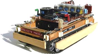
Figure 1.4 The expandable microrobot Prowler published in Sinclair projects, August 1983. Source: http://www.davidbuckley.net/DB/Prowler.htm.
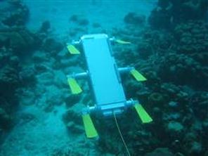
Figure 1.5 The AQUA robot can take pictures of coral reefs and other aquatic organisms returning home after completion of its tasks. Source: http://www.rutgersprep.org/kendall/7thgrade/cycleA_2008_09/zi/robo_AQUA.html.

Figure 1.6 The Genghis robot. Genghis has a special multilegged walking mode known as the “Genghis gait.” It is now retired at the Smithsonian Air Space Museum. Source: http://www.ai.mit.edu/prohects/genghis.
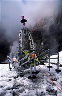
Figure 1.7 The Dante II explorer robot. Source: http://www.frc.ri.cmu.edu/robots/robs/photos/1994_DanteII.jpg.
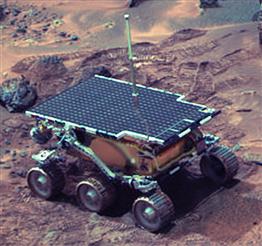
Figure 1.8 The NASA Sojourner robotic rover. Source: http://haberlesmeplatformu.blogspot.com/2010_04_01_archive.html.
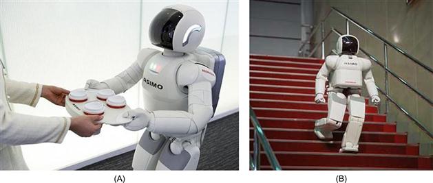
Figure 1.9 The Honda’s humanoid ASIMO. Source: http://www.gizmag.com/go/1765picture/2029; http://razorrobotics.com/safety.

Figure 1.10 The Rollin Justin robot mixing instant tea. Source: http://inventors.about.com/od/robotart/ig/Robots-and-Robotics/Rollin-Justin-Robot.htm.

Figure 1.11 (A) Seekur (350 kg, dimensions 1.4 m×1.3 m×1.1 m), (B) Pioneer 3D-X, and (C) PowerBot. Source: http://mobilerobots.com/ResearchRobots/ResearchRobots.aspx; http://www.conscious-robots.com/en/reviews/robots/mobilerobots-pioneer-3p3-dx-8.html.
1.3 Ground Robot Locomotion
Locomotion of ground mobile robots is distinguished in [4–15]1 :
1.3.1 Legged Locomotion
The wheel is a human invention, but the leg is a biological element. Locomotion of most of the highly developed animals is through legs. Biological multilegged organisms can move in diverse and difficult environments with obstacles, rough grounds, etc. Insects have very small size and weight and possess strong robustness that cannot be achieved by artificial creatures. To be useful in real-life tasks, a legged robot must be statically stable. This condition is satisfied if the center of gravity lies always within the polygon defined by the actual contact points with the ground. This can be achieved only if at each time three feet are in contact with the floor. Thus to guarantee statical stability four legs are at least needed. If the feet do not have contact points, but lines or planes of contact, this might not be true, and a statically stable robot may have only two legs. In practice, the contact of the robot body with the floor is a small region.
A legged robot is said to be dynamically stable if it is does not fall over, despite the fact that it is not statically stable. Legged robots are distinguished in two main categories:
Bipedal locomotion is standing on two legs, walking and running.
Humanoid robots are bipedal robots with an overall appearance based on that of the human body, that is, head, torso, legs, arms, and hands. Some humanoids may model only part of the body, for example, from waist up, such as in the NASA’s Robonaut, while others have also a “face” with “eyes” and “mouth.”
Robot bipedal locomotion needs complex interaction of mechanical and control system features. Humans are able to perform bipedal locomotion because their spines are s-curved and their heels are round. During locomotion the legs need to be lifted from and return to the ground. The sequence and way of placing and lifting each foot (in time and space), synchronized with the body motion so as to move from one place to another, is called gait.
The human gait involves the following distinct phases:
• Rocking back and forth between feet
• Pushing with the toe to sustain speed
• Combined interruption in rocking and ankle twist to turn
• Shortening and extending the knees to prolong the “forward fall”
The basic cycle of a gait is called a stride, which describes the complete cycle from one occurrence of a leg motion to its repetition. The fraction of a stride during which the foot is in on-state is called the duty factor. For statically stable walking the minimum duty factor needed is “3: (number of legs),” where 3 is the minimum number of feet in on-state to assure static stability. A walking gait is one where at least one foot is on the ground at any time. A running gait is occurring if for some time periods all feet are in off-state. Robots without static stability need higher energy to achieve dynamic stability, and extra stabilizing motions to prevent the body from falling over (in addition to useful/productive motions). The initial research on multilegged walking robots was focused on robot locomotion design for smooth or easy rough terrain, by passing simple obstacles, motion on soft ground, body maneuvering, and so on. These requirements can be realized via periodic gaits and binary (yes/no) contact information with the ground. Newer studies are concerned with multilegged robots that can move over an impassable road or an extremely complex terrain, such as mountain areas, ditches, trenches, earthquake damaged areas, etc. In these cases, additional capabilities are needed, as well as detailed support reactions and robot stability prediction. Figures 1.12–1.15 show three advanced multilegged robots with capabilities of the above type. The quadruped robot Kotetsu of Figure 1.12 is capable of adaptive walking using phase modulations based on leg loading/unloading.

Figure 1.12 The quadruped robot “Kotetsu” (leg length at standing 18–22 cm). Source: http://robotics.mech.kit.ac.jp/kimura/research/Quadruped/photo-movie-kotetsu-e.html.
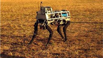
Figure 1.13 DARPA quadruped robot (LC3). Source: http://www.gizmag.com/darpa-lc3-robot-quadruped/14256/picture/111087.

Figure 1.14 Six-legged robot “SLAIR” capable of operating at “action level.” Source: http://www.uni-magdeburg.de/ieat/robotslab/images/Slair/CIMG1059.jpg.
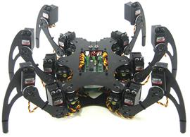
Figure 1.15 A typical example of hexabot robo-spider (Gadget Lab). Source: http://www.wired.com/gadgetlab/2010/04/gallery-spider-robot/2/.
1.3.2 Wheeled Locomotion
The maneuverability of a WMR depends on the wheels and drives used. The WMRs that have three DOF are characterized by maximal maneuverability which is needed for planar motions, such as operating on a warehouse floor, a road, a hospital, a museum, etc. Nonholonomic WMRs have less than three DOF in the plane, but they are simpler in construction and cheaper because less than three motors are used. A holonomic vehicle can travel in every direction and function in tight areas. This capability is called omnidirectionality. Balance is inherently assured in WMRs with three or more wheels. But in the case of m-wheel WMRs (m≥3) a suspension system must be used to assure that all wheels can have ground contact in rough terrains. The main problems in WMR design are the traction, maneuverability, stability, and control that depend on the wheel types and configurations (drives).
1.3.2.1 Wheel Types
The types of wheels used in WMRs are:
Conventional wheels: These wheels are distinguished in powered fixed wheels, castor wheels, and powered steering wheels. Powered fixed wheels (Figure 1.16A) are driven by motors mounted on fixed positions of the vehicle. Their axis of rotation has a fixed direction with respect to the platform’s coordinate frame. Castor wheels (Figure 1.16B) are not powered but they can also rotate freely about an axis perpendicular to their axis of rotation.
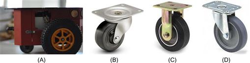
Figure 1.16 Conventional wheels (A) fixed wheel, (B) castor wheel, (C) powered steering wheel without any offset, and (D) power steering wheel with longitudinal offset.
Powered steering wheels have a driving motor for their rotation and can be steered about an axis perpendicular to their axis of rotation. They can be without offset (Figure 1.16C) or with offset (Figure 1.16D) in which case the axes of rotation and steering do not intersect. To achieve omnidirectionality with conventional castor and powered steering wheels some kind of motion redundancy should be used, for example, n-wheel drives (n>2) with all wheels driven and steered. Conventional wheels have higher load capacities and higher tolerance for ground irregularities compared to special wheel configurations. But due to their nonholonomic constraints are not truly omnidirectional wheels.
Special wheels: These wheels are designed such that to have activated traction in one direction and passive motion in another, thus allowing greater maneuverability in congested environments. We have three main types of special wheels:
The universal wheel provides a combination of constrained and unconstrained motion during turning. It contains small rollers around its outer diameter which are mounted perpendicular to the wheel’s rotation axis. This way the wheel can roll in the direction parallel to the wheel axis in addition to the normal wheel rotation (Figure 1.17).
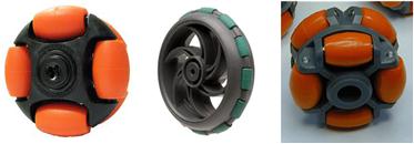
Figure 1.17 Three designs of universal wheel. Source: http://www.generationrobots.com/2-omni-directional-wheel-robot-v.ex-robotics,us,4,2165-Omni-Directional-Wheel-kit.cfm; http://www.rotacaster.com.au/robot-wheels.html; http://www-scf.usc.edu/~csci445_final_contest/SearchAndRescue/OtherContests/2004_contest_Fall_RobotSoccer/Locomotion/omni_4wheel_encoders/omni_drive.pdf.
The mecanum wheel is similar to the universal wheel except that the rollers are mounted at an angle α other than 90° (usually ±45°) (Figure 1.18).

Figure 1.18 (A) Mecanum wheel with α=45° (left wheel), (B) mecanum wheel with α=−45° (right wheel), and (C) an actual mecanum wheel. Source: http://www.aceize.com/node/562.
Figure 1.18A and B shows the omnidirectional wheel as it looks from the bottom (via a glass floor). The force F produced by the rotation of the wheel acts on the ground via the roller that has contact with the ground (which is assumed sufficiently flat without irregularities). At this roller, the force is decomposed in a force F1 parallel to the roller axis and a force F2 perpendicular to the roller axis. The force perpendicular to the roller axis produces a small roller rotation (speed vr), but the force parallel to the roller axis exerts a force on the wheel and thereby on the vehicle resulting in the hub speed vh. The actual velocity vt of the vehicle is the combination of vh and vr. Figure 1.18C shows a practical mecanum wheel.
The ball (or spherical) wheel places no direct constraints on the motion, that is, it is omnidirectional like castor or special universal and mecanum wheels. In other words, the rotational axis of the wheel can have any arbitrary direction. One way to achieve this is by using an active ring driven by a motor and gearbox to transmit power to the ball via rollers and friction, which is free to rotate in any direction instantaneously. Because of its difficult construction the ball wheel is very rarely used in practice. A type of ball wheel is shown in Figure 1.19.
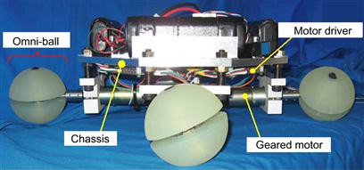
Figure 1.19 A practical implementation of a ball wheel. Source: http://www-hh.mech.eng.osaka-u.ac.jp/robotics/Omni-Ball_e.html.
1.3.2.2 Drive Types
The drives of WMRs are distinguished in:
Differential drive: This drive consists of two fixed powered wheels mounted on the left and right side of the robot platform. The two wheels are independently driven. One or two passive castor wheels are used for balance and stability. Differential drive is the simplest mechanical drive since it does not need rotation of a driven axis. If the wheels rotate at the same speed, the robot moves straight forward or backward. If one wheel is running faster than the other, the robot follows a curved path along the arc of an instantaneous circle. If both wheels are rotating at the same velocity in opposite directions, the robot turns about the midpoint of the two driving wheels. The above locomotion modes are illustrated in Figure 1.20. Clearly, this type of WMR cannot turn on the spot.
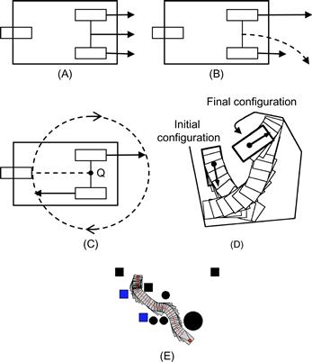
Figure 1.20 Locomotion possibilities of differential drive. (A) Straight path, (B) curved path, (C) circular path, (D) obstacle-free maneuvering to go from an initial to a final pose, and (E) maneuvering to go from an initial to a final pose while avoiding obstacles. Source: Colored picture, courtesy of N. Katevas.
The instantaneous center of curvature (ICC) of the WMR lies at the cross point of all axes of the wheels. ICC is the center of the circle with radius R depending on the speeds of the two wheels (Figure 1.21).

The radius R is determined by the relation: ![]() .
.
Therefore:
![]() (1.1)
(1.1)
When ![]() we have
we have ![]() (i.e., straight motion, and when
(i.e., straight motion, and when ![]() we have
we have ![]() (i.e., rotational motion).
(i.e., rotational motion).
Tricycle: This drive has a single wheel which is both driven (powered) and steered. For stability, two free-running (unpowered) fixed wheels in the back are used, in order to have always the three point contact required. The linear and angular velocities of the wheel are fully decoupled. For driving straight, the wheel is positioned in the middle position and driven at the desired speed (Figure 1.22A). When the front wheel is at an angle the vehicle follows a curved path (Figure 1.22B). If the front wheel is positioned at 90°, the robot will rotate following a circular path the center of which is in the middle point of the rear wheels and not in the robot’s geometric center (Figure 1.22C). This means that this WMR cannot turn on the spot. Nonholonomic WMRs (like differential drive or tricycle vehicles) cannot perform parallel parking directly but by a number of maneuvers with forward and backward movements as shown in Figure 1.22D.

Figure 1.22 Tricycle WMR locomotion modes (A–D), (E) A tricycle example. Source: http://www.asianproducts.com/product/A12391789884559774_p1240094409205655/cargo-tricycle(250cc).html.
Omnidirectional: This drive can be obtained using three, four, or more omnidirectional wheels as shown in Figure 1.23. WMRs with three wheels use universal wheels that have a 90° roller angle (Figure 1.17) as shown in Figure 1.23A. Omnidirectional WMRs with four wheels use mecanum wheels (Figure 1.18) in the configuration shown in Figure 1.23B.
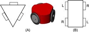
Figure 1.23 Omnidirectional WMRs. (A) Three-wheel case, (B) four-wheel case with roller angle different than 90° (typically α=±45°). Source: Colored picture, courtesy of Jahobr.
From the four wheels in Figure 1.24, two are called left-handed (L) wheels and the other two right-handed (R) wheels. The left-handed wheels have a roller angle α=45° and the right-handed ones an angle α=−45°. Therefore, the four-wheel omnidirectional WMRs have the typical structure shown in Figure 1.24.
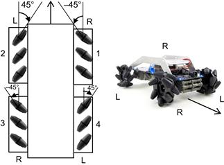
Figure 1.24 Standard setup of a four-mecanum-wheel omnidirectional WMR. Source: http://www.interhopen.com/download/pdf/pdfs_id/465/InTech-Omnidirectional_mobile_robot_design_and_implementation.pdf.
Figure 1.25 shows six basic motions of a four-wheel omnidirectional robot, namely (A) forward motion, (B) left sliding, (C) clockwise turning (on the spot), (D) backward motion, (E) right sliding, and (F) anticlockwise turning. The arrows on the left and the right side of the vehicle show the motion direction of the corresponding wheels.
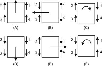
The arrows on the vehicle platform show the respective directions of the WMR motion, that is, for forward vehicle direction all wheels must move forward (Figure 1.25A), for left sliding wheels 1, 3 should move forward, and wheels 2, 4 backward, and so on. The locomotions shown in Figure 1.25 are obtained if all wheels move at the same speed. By varying the speed magnitude of the wheels one can realize WMR motion in any direction on the 2-D plane. A few cases are shown in Figure 1.26.
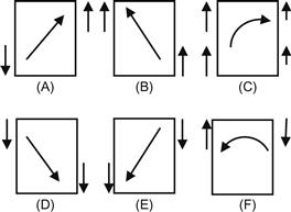
Figure 1.26 Six more locomotions: (A) forward-right, (B) forward-left, (C) curved right, (D) backward-right, (E) backward-left, and (F) lateral arc.
All locomotions of Figures 1.25 and 1.26 can be explained using the force or velocity diagrams of Figure 1.18A and B). For example, because of the symmetricity of left and right wheels (Figure 1.24), if all wheels are driven forward, there are four vectors pointing forward that are added up and four vectors pointing sideways, two to the left and two to the right, that cancel each other out. Thus, in overall the WMR moves forward. The L and R wheels may be interchanged (i.e., front wheels RL, back wheels LR). Again, with proper motion of the wheels all omnidirectional locomotion modes can be obtained with this setup too.
Synchro drive: This drive has three or more wheels that are mechanically coupled such that all of them rotate in the same direction at the same speed and pivot in unision about their own steering axes when perform a turn. This mechanical steering synchronization can be realized in several ways, for example, using a chain, a belt or gear drive. Actually, synchro drive is an extension of a single driven and steered wheel and so it still has only two DOF. But a synchro drive WMR is nearly a holonomous vehicle because it can move in any desired direction. However, it cannot drive and rotate at the same time. To change its driving from forward to sideways this WMR must stop and realign its wheels. Figure 1.27A shows pictorially how a three-wheel WMR with synchro drive is moving and rotated.
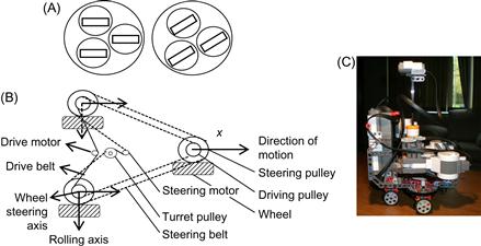
Figure 1.27 (A) Illustration of synchro drive WMR motion, (B) illustration of the two independent belt subsystems, and (C) a synchro drive WMR example. Source: http://members.efn.org/~kirbyf/05syncro/1.jpg.
Chain- or belt-based synchro drive presents lower steering accuracy and alignment. This problem does not occur if a gear drive is used. Actually, two independent motor-drive subsystems (operating with chain, belt, and gear) must be used; one for the steering and one for the driving shaft (Figure 1.27B).
Ackerman steering: This is the standard steering used in automobiles. It consists of two combined driven rear wheels and two combined steered front wheels. An Ackerman-steered vehicle can move straight (because the rear wheels are driven by a common axis), but cannot turn on the spot (it requires a certain minimum radius). The rear driving wheels experience slippage (when moving in curves).
Ackerman steering is designed so as to ensure that at turns the wheels of all axes have a common cross point (instantaneous center of rotation (ICR)), in order to avoid geometrically caused wheel slippage.
From Figure 1.28, we find the following relations:
![]()

which by elimination of L give:
![]()
![]() (1.2)
(1.2)
where ![]() is the vehicle’s actual steering angle and
is the vehicle’s actual steering angle and ![]() ,
, ![]() are the steering angles of the outer and inner wheel, respectively.
are the steering angles of the outer and inner wheel, respectively.
Figure 1.29 illustrates the constraint in the motion of an Ackerman-steered vehicle. There is a circular area on the left and on the right of its current position which is inaccessible to the vehicle. This is due to that the robot cannot turn (right or left) following a path with radius smaller than a minimum. Therefore, for parallel parking a considerable maneuvering is required.
Skid steering: This is a special implementation of differential drive and realized in track form on bulldozers and harmored vehicles. Its difference from a differential drive vehicle is the increased maneuverability in uneven terrains, and the higher friction which is due to its tracks and the multiple contact points with the terrain (rough or even). Figure 1.30A illustrates that the effective point contact for such a skid-steer robot is roughly constrained on either side by a rectangular uncertainty area which corresponds to the track footprint.

Figure 1.30 (A) Illustration of the effective contact point and (B) a typical tracked platform. Source: http://www.robotshop.com/Dr-robot-jaguar-tracked-mobile-platform-chassis-motors-3.html.
One can see from the concentric circles that for the vehicle to turn, a considerable slippage is needed. Figure 1.30B shows a typical tracked robotic platform that can carry a manipulator or special exploration equipment.
1.3.2.3 WMR Maneuverability
The maneuverability![]() of WMRs is defined as
of WMRs is defined as
![]() (1.3)
(1.3)
where ![]() is the degree of mobility, and
is the degree of mobility, and ![]() the degree of steerability.
the degree of steerability.
Degree of mobility: The degree of mobility ![]() is determined by the number of independent constraints that the type of wheels and their configuration impose on the motion ability of the robot. Constraints on the motion are imposed only by conventional wheels (fixed or steered). Omnidirectional wheels do not impose any constraint on the robot’s mobility. The best way to see the independent kinematic constraints of a WMR is by studying the geometric properties of the robot through the ICC or ICR. For example, a single conventional wheel cannot move laterally, that is, along the line determined by its axis of rotation. This line is called the zero motion line of the wheel. This means that the wheel can only move on an instantaneous circle of radius R with its center lying on the zero motion line. A bicycle has two wheels: the steered front wheel and the fixed wheel on the rear (Figure 1.31).
is determined by the number of independent constraints that the type of wheels and their configuration impose on the motion ability of the robot. Constraints on the motion are imposed only by conventional wheels (fixed or steered). Omnidirectional wheels do not impose any constraint on the robot’s mobility. The best way to see the independent kinematic constraints of a WMR is by studying the geometric properties of the robot through the ICC or ICR. For example, a single conventional wheel cannot move laterally, that is, along the line determined by its axis of rotation. This line is called the zero motion line of the wheel. This means that the wheel can only move on an instantaneous circle of radius R with its center lying on the zero motion line. A bicycle has two wheels: the steered front wheel and the fixed wheel on the rear (Figure 1.31).

Each wheel introduces a separate (independent) zero motion line. The two lines intersect at the ICR. In the case of a differential drive WMR (Figure 1.21) the zero motion lines of the two (common axis) wheels coincide and so they are not independent. This means that there is only one independent kinematic constraint. Any point on the common zero motion line can be an ICR. In the Ackerman steering, the WMR has four conventional wheels but two independent kinematic constraints (Figure 1.28). The two rear wheels impose a single constraint (as in the differential drive), and also the two front steered wheels impose a second single kinematic constraint, because they cross on an ICR lying on the zero motion line determined by the common axis rear wheels. The maximum degree of mobility ![]() is 3, which is true when no kinematic constraints are imposed. This is the case when all wheels of the WMR are omnidirectional. In general, the degree of mobility is equal to:
is 3, which is true when no kinematic constraints are imposed. This is the case when all wheels of the WMR are omnidirectional. In general, the degree of mobility is equal to:
![]() (1.4)
(1.4)
where ![]() is the number of independent constraints.
is the number of independent constraints.
Degree of steerability: The degree of steerability ![]() depends on the number of independently controllable steering parameters and lies in the interval
depends on the number of independently controllable steering parameters and lies in the interval ![]() . If no steerable wheels exist we have
. If no steerable wheels exist we have ![]() . The case
. The case ![]() holds only if the robot has no fixed standard wheels. In this case we can have a platform with two separate steerable conventional wheels (as e.g., in a 2-steer bicycle or 3-wheeled 2-steer WMR). Actually,
holds only if the robot has no fixed standard wheels. In this case we can have a platform with two separate steerable conventional wheels (as e.g., in a 2-steer bicycle or 3-wheeled 2-steer WMR). Actually, ![]() means that the WMR can place its ICR at any point of the plane. The most common case is
means that the WMR can place its ICR at any point of the plane. The most common case is ![]() which is obtained when the robot configuration has one or more steerable conventional wheels. A steered conventional wheel can decrease the robot’s mobility, but also can increase the steerability. In fact, although an instantaneous orientation of the wheel imposes a kinematic constraint its capability to change this orientation may allow additional trajectories. The maneuverability
which is obtained when the robot configuration has one or more steerable conventional wheels. A steered conventional wheel can decrease the robot’s mobility, but also can increase the steerability. In fact, although an instantaneous orientation of the wheel imposes a kinematic constraint its capability to change this orientation may allow additional trajectories. The maneuverability ![]() , the degree of mobility
, the degree of mobility ![]() and the degree of steerability
and the degree of steerability ![]() of some typical WMR configurations are shown in Table 1.1.
of some typical WMR configurations are shown in Table 1.1.

Two other characteristic parameters of WMRs are the “degrees of freedom” and the “differential degrees of freedom” (DDOF), which satisfy the relation:
![]()
The DDOF is equal to ![]() and represents the number of independent velocities that can be achieved. DOF represents the ability of a WMR to achieve various poses
and represents the number of independent velocities that can be achieved. DOF represents the ability of a WMR to achieve various poses ![]() in its environment (work space).
in its environment (work space).
A bicycle can achieve any pose ![]() on the plane by some maneuver and so it has DOF=3, but its DDOF is
on the plane by some maneuver and so it has DOF=3, but its DDOF is ![]() . An omnirobot, with three omnidirectional wheels, has
. An omnirobot, with three omnidirectional wheels, has ![]() , that is, DDOF=3, and also DOF=3. Similarly, a tricycle has
, that is, DDOF=3, and also DOF=3. Similarly, a tricycle has ![]() and DOF=3, because it can reach any
and DOF=3, because it can reach any ![]() by appropriate maneuvering.
by appropriate maneuvering.
A list of possible wheel drive configurations is as follows [7]:
• One traction wheel in the back, one steering wheel in the front (bicycle, motor cycle)
• Two-wheel differential drive with the center of mass, below the wheels’ axis (a balance controller is needed)
• Two-wheel differential drive centered with an omni wheel for stability (Nomad Scout robot)
• Three-wheel differential drive with an unpowered omni wheel, rear or front driven (typical indoor WMRs)
• Two connected powered wheels (differential) in the back, one free turning wheel in front
• One steered and driven wheel in front two free wheels in the back (e.g., Neptune)
• Three omnidirectional wheels (universal)
• Three synchronous powered and steered wheels (synchronous drive)
• Car-like WMR (rear-wheel driven)
• Car-like WMR (front-wheel driven)
• Four-wheel drive, four-wheel steering (Hyperion)
• Differential wheel drive in the back two omni wheels in front
• Four Swedish omnidirectional wheels ![]() (Uranus)
(Uranus)
A small set of modern WMRs falling in the above categories are shown in Figures 1.32–1.42.
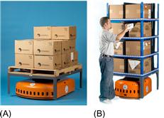
Figure 1.32 KIVA autonomous mobile robots. (A) Pallet and case handling, (B) Order fulfillment. Source: (A) www.kivasystems.com/solutions/picking/pick-from-pallets. (B) www.kivasystems.com/about-us-the-kiva-approach.
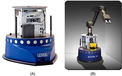
Figure 1.33 (A) SCITOS mobile general platform (SCITOS G5). (B) Robotic manipulator mounted on SCITOS G5.
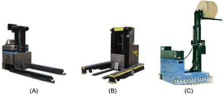
Figure 1.34 CORECON automated guided mobile robots (AGVs). (A) Horizontal roll handling, (B) low lift rear loader, and (C) high lift side loader. Source: www.coreconagvs.com/products.
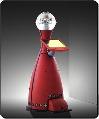
Figure 1.35 SCITOS mobile robot guide (it can provide users valuable information via speech or touch screen at any location). Source: http://www.expo21xx.com/automation21xx/13582_st3_mobile-robots/default.htm.
Figure 1.36 Mobile robot platform with spring-loaded castors for physical interaction with humans. Source: http://robot.kaist.ac.kr/paper/view.php?n=318.
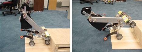
Figure 1.37 The CMU Rover 1 robot climbing a stair. Source: http://www.cs.cmu.edu/~myrover/Rover1/robot.htm.

Figure 1.38 The Nomad robot (CACS Louisiana University). Source: http://www.cacs.louisiana.edu/~sxg3148/nomad_pics/Nomad_robot_jpg.
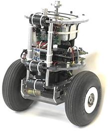
Figure 1.39 The NASA nBot (two-wheel balancing robot). Source: http://www.geology.smu.edu/~dpa-www/robot/nbot/nobot2/nb12.jpg.

Figure 1.40 The EPFL wheeled climbing “Octopus Robot” (43 cm×42 cm×23 cm). Source: http://www-robot.mes.titech.ac.jp/robot/walking/rollerwalker/roller_e.html.
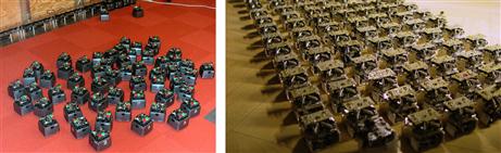
Figure 1.41 Robotic swarms showing a “collective behavior.” Source: http://www.humansinvent.com/#!/8878/swarm-robots-the-droid-workforce-of-the-future/.

Figure 1.42 The AMiR swarm robot. Source: http://www.swarmrobotic.com/Robot.htm.
Figure 1.42 shows the components of the AMiR swarm robot involving the main board, communication module, kinematic design, power module, and sensory system.
Figure 1.43 shows the miniature WMR “Khepera” used for research for more than 15 years. It was developed at the LAM laboratory in EPFL (Lausanne, Switzerland). The initial version of Khepera (Figure 1.43A) is 55 mm diameter and 30 mm high robot. It has appropriate sensors and actuators to ensure that it can be programmed to perform a large repertory of tasks. Khepera can run autonomously or tethered to a host computer. The newer versions of Khepera (K-II Version and K-III Version) are shown in Figure 1.43B and C).
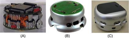
Figure 1.43 The evolution of Khepera WMR. (A) Original version, (B) Version K-II, (C) Version K-III. Source: http://mobotica.blogspot.com/2011/08khepera.html; www.k-team.com/mobile-robotics-products/KheperaII.
Khepera is able to move on a table top as well as on a room floor for performing real-world swarm robotics. To enable fast development of portable applications, Khepera III supports a standard Linux operating system.
Finally, Figure 1.44 shows the famous mecanum-wheeled omnidirectional WMR “Uranus.”

Figure 1.44 “Uranus” four-wheel omnidirectional robot. Source: http://www.cs.cmu.edu/afs/cs/user/gwp/www/robots/Uranus.jpg.
References
1. Freedman J. Robots through history: robotics New York, NY: Rosen Central; 2011.
2. Mayr O. The origins of feedback control Cambridge, MA: MIT Press; 1970.
3. Lazos C. Engineering and technology in ancient Greece Athens: Aeolos Editions; 1993.
4. Campion G, Bastin G, D’Andréa-Novel B. Structural properties and classification of kinematic and dynamic models of wheeled mobile robots. IEEE Trans Rob Autom. 1996;12(1):47–62.
5. Floreano D, Zufferey J-C. Robots mobiles. EPFL Course-Mobile Robots. <www.cs.cmu.edu/~gwp/robots/Uranus.html>.
6. Bekey G. Autonomous robots Cambridge, MA: MIT Press; 2005.
7. Siegwart R, Nourbakhsh I. Autonomous mobile robots Cambridge, MA: MIT Press; 2005.
8. Bräunl T. Embedded robotics: mobile robot design and applications with embedded systems Berlin: Springer; 2006; <http://newplans.net/RDB>.
9. Salih J, Rizon M, Yacacob S, Adom A, Mamat M. Designing omni-directional mobile robot with mecanum wheel. Am J Appl Sci. 2006;3(5):1831–1835.
10. West M, Asada H. Design of ball wheel mechanisms for omnidirectional vehicles with full mobility and invariant kinematics. J Mech Des. 1997;119:153–157.
11. Holland J-M. Rethinking robot mobility. Rob Age. 1988;7(1):26–30.
12. Duro JR, Santos J, Grana M. Biologically inspired robot behavior engineering Berlin/Heidelberg: Springer; 2002.
13. Katevas N, ed. Mobile robotics in healthcare. Amsterdam: IOS Press; 2001.
14. Tzafestas SG, ed. Autonomous mobile robots in health care services. J Intell Rob Syst. 1998;22(3–4):177–350 [special issue].
15. Fong T, Nourbakhsh IR, Dautenhahn K. A survey of socially interactive robots. Rob Auton Syst. 2003;42(3–4):143–166.
1UAVs and AUVs will not be studied in this book.