
Mobile Manipulator Modeling and Control
Mobile manipulators (MMs) are robotic systems consisting of articulated arms (manipulators) mounted on holonomic or nonholonomic mobile platforms. They provide the dexterity of the former and the workspace extension of the latter. They are able to reach and work over objects that are initially outside the working space of the articulated arm. Therefore, MMs are appealing for many applications, and today they constitute the main body of service robots. One of the principal and most challenging problems in MMs research is to design accurate controllers for the entire system.
The objectives of this chapter are (i) to present the Denavit–Hartenberg method of articulated robots’ kinematic modeling, and provide a practical method for inverse kinematics, (ii) to study the general kinematic and dynamic models of MMs, (iii) to derive the kinematic and dynamic models of a differential drive and a three-wheel omnidirectional MM, with two-link and three-link mounted articulated arms, respectively, (iv) to derive a computed-torque controller for the above differential-drive MM, and a sliding-mode controller for the three-wheel omnidirectional MM, and (v) to discuss some general issues of MM visual-based control, including a particular indicative example of hybrid coordinated (feedback/open-loop) visual control, and an omnidirectional (catadioptric) visual robot control example.
Keywords
Mobile manipulator modeling; mobile manipulator control; manipulability; omnidirectional mobile manipulator modeling; nonholonomic mobile manipulator modeling; differential-drive mobile manipulator control; full-state mobile manipulator visual control; mobile manipulator control; maximum manipulability
10.1 Introduction
Mobile manipulators (MMs) are robotic systems consisting of articulated arms (manipulators) mounted on holonomic or nonholonomic mobile platforms. They provide the dexterity of the former and the workspace extension of the latter. They are able to reach and work over objects that are initially outside the working space of the articulated arm. Therefore, MMs are appealing for many applications, and today they constitute the main body of service robots [1–27]. One of the principal and most challenging problems in MMs research is to design accurate controllers for the entire system. Due to the strong interaction and coupling of the mobile platform subsystem and the manipulator arm(s) mounted on the platform, a proper coordination between the respective controllers is needed [18,23]. However, in the literature there are also available unified control design methods that treat the whole system using the full-state MM model [3,10,22,24]. In either case the control methods studied in this book (computed-torque control, feedback linearizing control, robust sliding-mode or Lyapunov-based control, adaptive control, and visual-based control) can be employed and combined.
The objectives of this chapter are as follows:
• To present the Denavit–Hartenberg method of articulated robots’ kinematic modeling, and provide a practical method for inverse kinematics
• To study the general kinematic and dynamic models of MMs
• To derive the kinematic and dynamic model of a differential drive, and a three-wheel omnidirectional MM, with two-link and three-link mounted articulated arms, respectively
• To derive a computed-torque controller for the above differential-drive MM, and a sliding-mode controller for the three-wheel omnidirectional MM
• To discuss some general issues of MM visual-based control, including a particular indicative example of hybrid coordinated (feedback/open-loop) visual control and a panoramic visual servoing example.
10.2 Background Concepts
Here, the following aspects which will be used in the chapter are considered:
• The Denavit–Hartenberg direct manipulator kinematics method
• A general method for inverse manipulator kinematics
• The manipulability measure concept
• The two-link manipulator’s direct and inverse kinematic model and manipulability measure.
10.2.1 The Denavit–Hartenberg Method
The Denavit–Hartenberg method provides a systematic procedure for determining the position and orientation of the end-effector of an n-joint robotic manipulator, that is, for computing ![]() in (2.18).
in (2.18).
Consider a link ![]() that lies between the joints
that lies between the joints ![]() and
and ![]() of a robot as shown in Figure 10.1.
of a robot as shown in Figure 10.1.
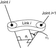
Each link is described by the distance ![]() between the (possibly nonparallel) axes
between the (possibly nonparallel) axes ![]() and
and ![]() of the two joints, and the rotation angle
of the two joints, and the rotation angle ![]() from the axis
from the axis ![]() to the axis
to the axis ![]() with respect to the common normal of the two axes. Each joint (prismatic or rotary) is driven by a motor (translational or rotational) that produces the motion of link
with respect to the common normal of the two axes. Each joint (prismatic or rotary) is driven by a motor (translational or rotational) that produces the motion of link ![]() . In overall, the robotic arm has
. In overall, the robotic arm has ![]() joints and
joints and ![]() links. The functional relation of the end-effector and the displacements of the joints can be found using the convention of parameters shown in Figure 10.2, called the Denavit–Hartenberg parameters.
links. The functional relation of the end-effector and the displacements of the joints can be found using the convention of parameters shown in Figure 10.2, called the Denavit–Hartenberg parameters.
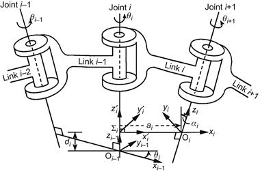
These parameters refer to the relative position of the coordinate frames ![]() and
and ![]() , and are the following:
, and are the following:
• The length ![]() of the common normal
of the common normal ![]()
• The distance ![]() between the origin of
between the origin of ![]() and the point
and the point ![]()
• The angle ![]() between the joint
between the joint ![]() (i.e., the axis
(i.e., the axis ![]() ) and the axis
) and the axis ![]() in the positive (clockwise) direction
in the positive (clockwise) direction
• The angle ![]() between the axis
between the axis ![]() and the common normal (i.e., rotation about the axis
and the common normal (i.e., rotation about the axis ![]() ) in the positive direction.
) in the positive direction.
On the basis of the above, the transfer from the frame ![]() to the frame
to the frame ![]() can be done in four steps:
can be done in four steps:
Step 1: Rotation of frame ![]() about the axis
about the axis ![]() by an angle
by an angle ![]() .
.
Step 2: Translation of frame ![]() along the axis
along the axis ![]() by
by ![]() .
.
Step 3: Translation of the rotated axis ![]() (which now coincides with
(which now coincides with ![]() ) along the common normal by
) along the common normal by ![]() .
.
Denoting by ![]() the result of steps 3 and 4 and by
the result of steps 3 and 4 and by ![]() the result of steps 1 and 2, the overall result of steps 1 through 4 is given by:
the result of steps 1 and 2, the overall result of steps 1 through 4 is given by:
 (10.1)
where ![]() gives the position and orientation of the frame
gives the position and orientation of the frame ![]() with respect to the frame
with respect to the frame ![]() . The first three columns of
. The first three columns of ![]() contain the direction cosines of the axes of frame
contain the direction cosines of the axes of frame ![]() , whereas the fourth column represents the position of frame
, whereas the fourth column represents the position of frame ![]() .
.
In general, the displacement of joint ![]() is denoted as
is denoted as ![]() , where:
, where:
The position and orientation of link ![]() with respect to link
with respect to link ![]() is a function of
is a function of ![]() , that is,
, that is, ![]() .
.
The kinematic equation of a robotic arm gives the position and orientation of the last link with respect to the coordinate frame of the base, and obviously contains all generalized variables ![]() of the joints. Figure 10.3 shows pictorially the consecutive coordinate frames from the base up to the end-effector of the serial robotic kinematic chain.
of the joints. Figure 10.3 shows pictorially the consecutive coordinate frames from the base up to the end-effector of the serial robotic kinematic chain.

According to Eq. (2.18), the matrix ![]() given by:
given by:
![]() (10.2)
(10.2)
represents the position and orientation of the end-effector (which is the final link with respect to the base). It is now easy to determine ![]() for all types of robots (Figure 10.4) using Eq. (10.2).
for all types of robots (Figure 10.4) using Eq. (10.2).

10.2.2 Robot Inverse Kinematics
In the direct kinematics problem we are finding ![]() knowing the values of
knowing the values of ![]() . In the inverse kinematics problem we do the converse, that is, given
. In the inverse kinematics problem we do the converse, that is, given ![]() we determine
we determine ![]() by solving (10.2) with respect to
by solving (10.2) with respect to ![]() .
.
The direct kinematics Eq. (10.2) can be written in the vectorial form:
![]() (10.3)
(10.3)
where ![]() is the six-dimensional vector:
is the six-dimensional vector:
 (10.4)
of the end-effector’s position ![]() and orientation
and orientation ![]() ,
, ![]() is a six-dimensional nonlinear column vectorial function, and
is a six-dimensional nonlinear column vectorial function, and
![]() (10.5)
(10.5)
Therefore, the inverse kinematics equation is:
![]() (10.6)
(10.6)
where ![]() denotes the usual inverse function of
denotes the usual inverse function of ![]() .
.
A straightforward practical method for inverting the kinematic Eq. (10.2) is the following. We start from:
![]()
and obtain the following sequence of equations:
 (10.7)
The elements of the left-hand sides of these equations are functions of the elements of ![]() and the first
and the first ![]() variables of the robot. The elements of the right-hand sides are constants or functions of the variables
variables of the robot. The elements of the right-hand sides are constants or functions of the variables ![]() . From each matrix equation we get 12 equations, that is, one equation for each of the elements of the four vectors
. From each matrix equation we get 12 equations, that is, one equation for each of the elements of the four vectors ![]() and
and ![]() . From these equations we can determine the values of
. From these equations we can determine the values of ![]() of the robot.
of the robot.
Although the solution of the direct kinematics problem is unique, it is not so for the inverse kinematics problem, because of the presence of trigonometric functions. In some cases, the solution can be found analytically, but, in general, the solution can only be found approximately using some approximate numerical method and the computer. Also, if the robot has more than six degrees of freedom (i.e., if we have a redundant robot), there are infinitely many solutions to ![]() that lead to the same position and orientation of the end-effector.
that lead to the same position and orientation of the end-effector.
10.2.3 Manipulability Measure
An important factor that determines the ease of arbitrarily changing the position and orientation of the end-effector by a manipulator is the so-called manipulability measure. Other factors are the size and geometric shape of the workspace envelope, the accuracy and repeatability, the reliability and safety, etc. Here, we will examine the manipulability measure, which was fully studied by Yoshikawa.
Given a manipulator with ![]() degrees of freedom, the direct kinematics equation is given by Eq. (10.3):
degrees of freedom, the direct kinematics equation is given by Eq. (10.3):
![]()
where ![]() is the m-dimensional vector
is the m-dimensional vector ![]() of the end-effector’s position
of the end-effector’s position ![]() and orientation vector
and orientation vector ![]() . Differentiating this relation we get the well-known differential kinematics model:
. Differentiating this relation we get the well-known differential kinematics model:
![]()
where ![]() is the manipulator’s Jacobian. This relation relates the velocity
is the manipulator’s Jacobian. This relation relates the velocity ![]() of the manipulator joints with the velocity of the end-effector, that is, the screw of the robot.
of the manipulator joints with the velocity of the end-effector, that is, the screw of the robot.
The set of all end-effector velocities that are realizable by joint velocities such as:
![]()
is an ellipsoid in the m-dimensional Euclidean space where ![]() is the dimensionality of
is the dimensionality of ![]() . The maximum speed of motion of the end-effector is along the major axis, and the minimum speed along the minor axis of this ellipsoid is called manipulability ellipsoid. One can show that the manipulability ellipsoid is the set of all
. The maximum speed of motion of the end-effector is along the major axis, and the minimum speed along the minor axis of this ellipsoid is called manipulability ellipsoid. One can show that the manipulability ellipsoid is the set of all ![]() that satisfy:
that satisfy:
![]()
for all ![]() in the range of
in the range of ![]() . Indeed, by using the relation
. Indeed, by using the relation ![]() (
(![]() =arbitrary constant vector) and the equality
=arbitrary constant vector) and the equality ![]() , we get
, we get
Thus, if ![]() , then
, then ![]() . Conversely, if we choose an arbitrary
. Conversely, if we choose an arbitrary ![]() such that
such that ![]() , then there exists a vector
, then there exists a vector ![]() such that
such that ![]() , that is,
, that is, ![]() . Then, we find that:
. Then, we find that:
![]()
![]()
In nonsingular configurations, the manipulability ellipsoid is given by:
![]()
The manipulability measure ![]() of the manipulator is defined as:
of the manipulator is defined as:
![]()
which for ![]() reduces to:
reduces to:
![]()
In this case, the set of all velocities that are implemented by a velocity ![]() of the joints such that:
of the joints such that:
![]()
is a parallelepiped in m-dimensional space with a volume of ![]() . This means that the measure
. This means that the measure ![]() is proportional to the volume of the parallelepiped, a fact that provides a physical representation of the manipulability measure.
is proportional to the volume of the parallelepiped, a fact that provides a physical representation of the manipulability measure.
10.2.4 The Two-Link Planar Robot
10.2.4.1 Kinematics
Consider the planar robot of Figure 10.5.
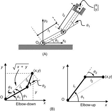
Figure 10.5 (A) Planar two degrees of freedom robot and (B) geometry for finding the inverse kinematic model (elbow-down, elbow-up).
The kinematic model of this robot can be found by simple trigonometric calculation. Referring to Figure 10.5 we readily obtain the direct kinematic model:
![]() (10.8a)
(10.8a)
that is:
![]() (10.8b)
(10.8b)
To derive the inverse kinematic model ![]() we work on Figure 10.5B.
we work on Figure 10.5B.
Thus, using the cosine rule we find:
![]()
from which the angle ![]() is found to be:
is found to be:
![]() (10.9a)
(10.9a)
The angle ![]() is equal to:
is equal to:
![]()
where:
![]()
Therefore:
![]() (10.9b)
(10.9b)
Actually, we have two configurations that lead to the same position ![]() of the end-effector, viz., elbow-down and elbow-up as shown in Figure 10.5. When
of the end-effector, viz., elbow-down and elbow-up as shown in Figure 10.5. When ![]() , that can be obtained if
, that can be obtained if ![]() , the ratio
, the ratio ![]() is not defined. If
is not defined. If ![]() , the base
, the base ![]() can be reached for all
can be reached for all ![]() . Finally, when a point is out of the workspace, the inverse kinematic problem has no solution.
. Finally, when a point is out of the workspace, the inverse kinematic problem has no solution.
The differential kinematics equation is:
![]()
Here, the Jacobian matrix ![]() is obtained by differentiating Eq. (10.8a), that is:
is obtained by differentiating Eq. (10.8a), that is:
![]() (10.10)
(10.10)
The inverse of ![]() is found to be:
is found to be:
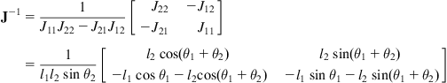 (10.11)
Thus, the inverse differential kinematics equation of the robot is:
![]() (10.12)
(10.12)
The singular (degenerate) configurations occur when ![]() , that is, when
, that is, when ![]() or
or ![]() . These two configurations correspond, respectively to the origin
. These two configurations correspond, respectively to the origin ![]() and to the full extension (i.e., when the robot end-effector is at the boundary of the workspace) (see Figure 10.5B).
and to the full extension (i.e., when the robot end-effector is at the boundary of the workspace) (see Figure 10.5B).
10.2.4.2 Dynamics
To derive the dynamic model of the robot we apply directly the Lagrange method. Consider the notation of Figure 10.6.
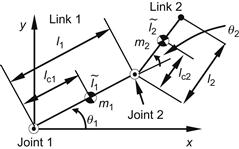
The symbols ![]() and
and ![]() have the usual meaning,
have the usual meaning, ![]() and
and ![]() are the masses of the two links (concentrated at their centers of gravity), and
are the masses of the two links (concentrated at their centers of gravity), and ![]() and
and ![]() are the lengths of the links. The symbol
are the lengths of the links. The symbol ![]() denotes the distance of the ith-link’s center of gravity (COG) from the axis of the joint
denotes the distance of the ith-link’s center of gravity (COG) from the axis of the joint ![]() , and
, and ![]() denotes the moment of inertia of link
denotes the moment of inertia of link ![]() with respect to the axis passing via the COG of this link and is perpendicular to the plane
with respect to the axis passing via the COG of this link and is perpendicular to the plane ![]() (parallel to the axis
(parallel to the axis ![]() ). Here,
). Here, ![]() and
and ![]() , and the kinematic and potential energies of the links 1 and 2 are given by:
, and the kinematic and potential energies of the links 1 and 2 are given by:
![]() (10.13a)
(10.13a)
![]() (10.13b)
(10.13b)
where ![]() is the position vector of the COG of link 2 with:
is the position vector of the COG of link 2 with:
![]()
and ![]() .
.
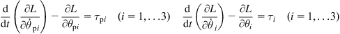
Using the Lagrangian function of the robot, ![]() , we find the equations:1
, we find the equations:1
![]() (10.14)
(10.14)
with:
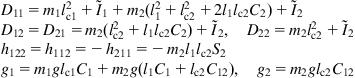 (10.15)
where ![]() and
and ![]() are the external torques applied to joints 1 and 2. The coefficient
are the external torques applied to joints 1 and 2. The coefficient ![]() is the effective inertia of the joint
is the effective inertia of the joint ![]() ,
, ![]() is the coupling inertia of joints
is the coupling inertia of joints ![]() and
and ![]() ,
, ![]() is the coefficient of centrifugal force,
is the coefficient of centrifugal force, ![]() is the coefficient of Coriolis acceleration of the joint
is the coefficient of Coriolis acceleration of the joint ![]() due to the velocities of the joints
due to the velocities of the joints ![]() and
and ![]() , and
, and ![]() represent the torques due to gravity. The dynamic relations in Eqs. (10.14) and (10.15) can be written in the standard compact form:
represent the torques due to gravity. The dynamic relations in Eqs. (10.14) and (10.15) can be written in the standard compact form:
![]() (10.16a)
(10.16a)
![]() (10.16b)
(10.16b)
 (10.16c)
where ![]() denotes a column vector with elements
denotes a column vector with elements ![]() . In the special case, where the link masses
. In the special case, where the link masses ![]() and
and ![]() are assumed to be concentrated at the end of each link, we have
are assumed to be concentrated at the end of each link, we have ![]() and
and ![]() . It is easy to verify the properties described by Eqs. (3.12) and (3.13) and the antisymmetricity of
. It is easy to verify the properties described by Eqs. (3.12) and (3.13) and the antisymmetricity of ![]() , where
, where ![]() is the total kinetic energy
is the total kinetic energy ![]() of the robot.
of the robot.
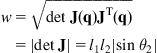
10.2.4.3 Manipulability Measure
If we use the position ![]() of the end-effector as the vector
of the end-effector as the vector ![]() , then (see (10.10)):
, then (see (10.10)):
![]()
and so the manipulability measure ![]() is:
is:
![]()
Thus, the optimal configurations of the manipulator, at which ![]() is maximum, are:
is maximum, are: ![]() for any
for any ![]() and
and ![]() . If the lengths
. If the lengths ![]() and
and ![]() are specified under the condition of constant total length (i.e.,
are specified under the condition of constant total length (i.e., ![]() ), then the manipulability measure takes its maximum when
), then the manipulability measure takes its maximum when ![]() for any
for any ![]() and
and ![]() .
.
10.3 MM Modeling
The total kinematic and dynamic models of an MM are complex and strongly coupled, combining the models of the mobile platform and the fixed robotic manipulator [1,3,7]. Today, MMs are in use with differential-drive, tricycle, car-like, and omnidirectional platforms that offer maximum maneuverability.
10.3.1 General Kinematic Model
Consider the MM of Figure 10.7 which has a differential-drive platform and a multilink robotic manipulator.
Here, we have the following four coordinate frames:
![]() is the world coordinate frame,
is the world coordinate frame,
![]() is the platform coordinate frame,
is the platform coordinate frame,
Then, the manipulator’s end-effector position/orientation with respect to ![]() is given by (see Eq. (10.2)):
is given by (see Eq. (10.2)):
![]() (10.17)
(10.17)
In vectorial form, the end-effector position/orientation vector ![]() in world coordinates has the form:
in world coordinates has the form:
![]() (10.18)
(10.18)
where:
![]()
![]()
![]()
Therefore, differentiating Eq. (10.18) with respect to time we get:
![]() (10.19)
(10.19)
where ![]() is given by the kinematic model of the platform (see (6.1)):
is given by the kinematic model of the platform (see (6.1)):
![]() (10.20a)
(10.20a)
and ![]() by the manipulator’s kinematic model. Assuming that the manipulator is constraint-free, we can write:
by the manipulator’s kinematic model. Assuming that the manipulator is constraint-free, we can write:
![]() (10.20b)
(10.20b)
where ![]() is the vector of manipulator’s joint commands. Combining Eqs. (10.19), (10.20a), and (10.20b) we get the overall kinematic model of the MM:
is the vector of manipulator’s joint commands. Combining Eqs. (10.19), (10.20a), and (10.20b) we get the overall kinematic model of the MM:
 (10.21a)
where:
 (10.21b)
Equation (10.21a) represents the total kinematic model of the MM from the inputs to the end-effector (task) variables.
Actually, in the present case the system is subject to the nonholonomic constraint:
![]() (10.22)
(10.22)
where ![]() cannot be eliminated by integration. Therefore,
cannot be eliminated by integration. Therefore, ![]() should involve a row representing this constraint. Since the dimensionality
should involve a row representing this constraint. Since the dimensionality ![]() of the control input vector
of the control input vector ![]() is less than the total number
is less than the total number ![]() of variables (degrees of freedom) to be controlled, the system is always underactuted.
of variables (degrees of freedom) to be controlled, the system is always underactuted.
10.3.2 General Dynamic Model
The Lagrange dynamic model of the MM is given by Eq. (3.16):
![]() (10.23)
(10.23)
where ![]() is given by Eq. (10.22). This model contains two parts, namely:
is given by Eq. (10.22). This model contains two parts, namely:
Platform Part
![]()
Manipulator Part
![]()
where the index ![]() refers to the platform and
refers to the platform and ![]() to the manipulator, and the symbols have the standard meaning. Appling the technique of Section 3.2.4 we eliminate the nonholonomic constraint
to the manipulator, and the symbols have the standard meaning. Appling the technique of Section 3.2.4 we eliminate the nonholonomic constraint ![]() , and get the reduced (unconstrained) model of the form of Eqs. (3.19a) and (3.19b):
, and get the reduced (unconstrained) model of the form of Eqs. (3.19a) and (3.19b):
![]() (10.24)
(10.24)
where:
![]()
and ![]() , and
, and ![]() are given by the combination of the respective terms in the platform and manipulator parts (the details of derivation are straightforward and are left as exercise).
are given by the combination of the respective terms in the platform and manipulator parts (the details of derivation are straightforward and are left as exercise).
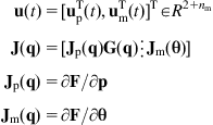
10.3.3 Modeling a Five Degrees of Freedom Nonholonomic MM
Here, the above general methodology will be applied to the MM of Figure 10.8 which consists of a differential-drive mobile platform and a two-link planar manipulator [3,22].
10.3.3.1 Kinematics
Without loss of generality, the COG ![]() is assumed to coincide with the rotation point
is assumed to coincide with the rotation point ![]() (midpoint of the two wheels), that is,
(midpoint of the two wheels), that is, ![]() . The nonholonomic constraint of the platform is:
. The nonholonomic constraint of the platform is:
![]()
This constraint, when expressed at the base ![]() of the manipulator, becomes:
of the manipulator, becomes:
![]()
where ![]() is the distance between the points
is the distance between the points ![]() and
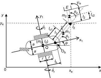
and ![]() . The kinematic equations of the wheeled mobile robot (WMR) platform (at the point
. The kinematic equations of the wheeled mobile robot (WMR) platform (at the point ![]() ) are:
) are:
 (10.25)
which are written in the Jacobian form:
![]()
where:
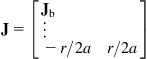
 (10.26)
![]() (10.27)
(10.27)
The kinematic parameters of the two-link manipulator are those of Figure 10.6, where now its first joint has linear velocity ![]() . The linear velocity
. The linear velocity ![]() of the end-effector is given by:
of the end-effector is given by:
![]() (10.28a)
(10.28a)
where ![]() :
:
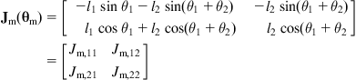 (10.28b)
is the Jacobian matrix of the manipulator with respect to its base coordinate frame (see Eq. (10.10)). Here, ![]() is given by the third part of Eq. (10.25), that is,
is given by the third part of Eq. (10.25), that is, ![]() . Thus:
. Thus:
![]() (10.29a)
(10.29a)
and so:
![]() (10.29b)
(10.29b)
The overall kinematic equation of the MM is:
![]() (10.30a)
(10.30a)
where:
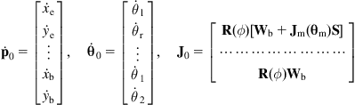 (10.30b)
If the mobile platform of the MM is of the tricycle or car-like type shown in Figure 2.8 or Figure 2.9, its position/orientation is described by four variables ![]() and
and ![]() , and the kinematic Eq. (2.45) or Eq. (2.53) is enhanced as in Eq. (10.25) with the
, and the kinematic Eq. (2.45) or Eq. (2.53) is enhanced as in Eq. (10.25) with the ![]() terms. The overall kinematic model of the MM is found by the same procedure.
terms. The overall kinematic model of the MM is found by the same procedure.
10.3.3.2 Dynamics
Assuming that the moment of inertia of the passive wheel is negligible, the Lagrangian of the MM is found to be:
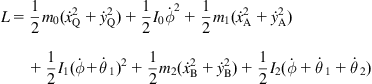 (10.31)
![]() are mass and moment of inertia of the platform,
are mass and moment of inertia of the platform,
![]() are masses and moments of inertia of links 1 and 2, respectively,
are masses and moments of inertia of links 1 and 2, respectively,
Using the Lagrangian (10.31) we derive the dynamic model of Eq. (10.23), with the nonholonomic constraint:
![]() (10.32)
(10.32)
Now, using the transformation ![]() with
with ![]() , where:
, where:
![]()
and ![]() is selected as:
is selected as:
 (10.33)
where ![]() is the
is the ![]() unit matrix, and
unit matrix, and
 (10.34)
the constrained Lagrangian model is reduced, as usual, to the unconstrained form (10.24).
Example 10.1
It is desired to investigate the manipulability measure of an MM and compute it for a five degrees of freedom MM.
Solution
The manipulability measure is given by:
![]()
or ![]() , if
, if ![]() is square. Let us define by
is square. Let us define by ![]() , the
, the ![]() larger numbers
larger numbers ![]() , where
, where ![]() is the ith eigenvalue of the matrix
is the ith eigenvalue of the matrix ![]() . Then, the above definition of
. Then, the above definition of ![]() reduces to:
reduces to:
![]()
The numbers ![]() are known as singular values of
are known as singular values of ![]() , and form the matrix
, and form the matrix ![]() :
:

which defines the singular value decomposition ![]() of
of ![]() with
with ![]() and
and ![]() being orthogonal matrices of dimensionality
being orthogonal matrices of dimensionality ![]() and
and ![]() respectively. The principal axes of the manipulability ellipsoid are
respectively. The principal axes of the manipulability ellipsoid are ![]() where
where ![]() are the columns of
are the columns of ![]() . Some other definitions of the manipulability measure are:
. Some other definitions of the manipulability measure are:
(i) ![]() : The ratio of the minimum and maximum singular values (radii) of the manipulator ellipsoid. This provides only qualitative information about the manipulability of the robot. If
: The ratio of the minimum and maximum singular values (radii) of the manipulator ellipsoid. This provides only qualitative information about the manipulability of the robot. If ![]() , then the ellipsoid is a sphere and the robot has the same manipulability in all directions.
, then the ellipsoid is a sphere and the robot has the same manipulability in all directions.
(ii) ![]() : The minimum radius which gives the upper bound of the velocity of the end-effector motion in any direction.
: The minimum radius which gives the upper bound of the velocity of the end-effector motion in any direction.
(iii) ![]() : The radius of the sphere that has the same volume of the manipulability ellipsoid.
: The radius of the sphere that has the same volume of the manipulability ellipsoid.
(iv) ![]() : The generalized concept of eccentricity of an ellipse.
: The generalized concept of eccentricity of an ellipse.
Consider the manipulability definition via ![]() . In the present case, the total Jacobian matrix of the MM is given by Eqs. (10.21a) and (10.21b), and represents the transformation from:
. In the present case, the total Jacobian matrix of the MM is given by Eqs. (10.21a) and (10.21b), and represents the transformation from:
to
![]()
where ![]() are the position coordinates, and
are the position coordinates, and ![]() the orientation angle of the end-effector. Then:
the orientation angle of the end-effector. Then:
![]()
and the MM manipulability ellipsoid is defined by:
Unfortunately, in most cases it is not possible to decouple ![]() and
and ![]() in computing the ellipsoid
in computing the ellipsoid ![]() . Now, consider the five-link MM of Figure 10.8. It is straightforward to find that:
. Now, consider the five-link MM of Figure 10.8. It is straightforward to find that:


Consider the manipulability measure ![]() which gives information on the shape of the ellipses. As
which gives information on the shape of the ellipses. As ![]() tends to zero, that is,
tends to zero, that is, ![]() the ellipsoid tends to a sphere and the attainable end-effector speeds tend to be the same in all directions. Actually, they can be equal (isotropic) when
the ellipsoid tends to a sphere and the attainable end-effector speeds tend to be the same in all directions. Actually, they can be equal (isotropic) when ![]() , for a given bounded velocity control signal.
, for a given bounded velocity control signal.
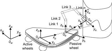
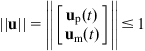
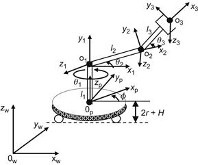
10.3.4 Modeling an Omnidirectional MM
Here, the kinematic and dynamic model of the MM shown in Figure 10.9 will be derived. This MM involves a three-wheel omnidirectional platform (with orthogonal wheels) and a 3D manipulator [8,11].
10.3.4.1 Kinematics
As usual, the kinematic model of the MM is found by combining the kinematic models of the platform and the manipulator.
The workspace of the robot is described by the world coordinate frame ![]() . The platform’s coordinate frame
. The platform’s coordinate frame ![]() has its origin at the COG of the platform, and the wheels have a radius
has its origin at the COG of the platform, and the wheels have a radius ![]() , an angle
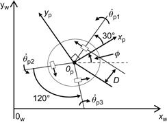
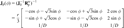
, an angle ![]() between them, and a distance D from the platform’s COG. The kinematic model of the robot was derived in Section 2.4. For the platform shown in Figure 10.9, the model given by Eqs. (2.74a) and (2.74b) becomes:
between them, and a distance D from the platform’s COG. The kinematic model of the robot was derived in Section 2.4. For the platform shown in Figure 10.9, the model given by Eqs. (2.74a) and (2.74b) becomes:
that is,
![]() (10.35)
(10.35)
where ![]() are the angular velocities of the wheels,
are the angular velocities of the wheels, ![]() the rotational angle between
the rotational angle between ![]() and
and ![]() axes, and
axes, and ![]() are the components of the platform’s velocity expressed in the platform’s (moving) coordinate system. The coordinate transformation matrix between the world and the platform coordinate frames is:
are the components of the platform’s velocity expressed in the platform’s (moving) coordinate system. The coordinate transformation matrix between the world and the platform coordinate frames is:
 (10.36)
Thus, the relation between ![]() and
and ![]() is
is
![]() (10.37)
(10.37)
Inverting Eq. (10.37) we get the direct differential kinematic model of the robot from ![]() to
to ![]() as:
as:
![]() (10.38a)
(10.38a)
 (10.38b)
Now, the platform’s kinematic model of Eq. (10.38a) will be integrated with the manipulator’s kinematic model (see Figure 10.10).
From Figure 10.9 we get:
 (10.39)
where ![]() is the height of the platform. Now, differentiating Eq. (10.39) and using Eqs. (10.38a) and (10.38b) we get:
is the height of the platform. Now, differentiating Eq. (10.39) and using Eqs. (10.38a) and (10.38b) we get:
![]() (10.40)
(10.40)
where: ![]() and
and ![]() is a
is a ![]() matrix with columns:
matrix with columns:
 (10.41)
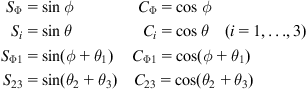
The notations used in the above expressions are:
10.3.4.2 Dynamics
To find the dynamic model of the MM, the local coordinate frames are employed according to the Denavit–Hartenberg convention. Figure 10.10 shows all the coordinate frames involved. Using the above notations, we obtain the following rotational matrices:

Now, for each rigid body composing the MM, the kinetic and potential energies are found. Then the Lagrangian function ![]() is built. Finally, the equations of the generalized forces are calculated using the Lagrangian function:
is built. Finally, the equations of the generalized forces are calculated using the Lagrangian function:
where ![]() are the generalized torques for the wheel actuators that drive the platform, and
are the generalized torques for the wheel actuators that drive the platform, and ![]() are the generalized torques for the joint actuators that drive the links of the manipulator. The parameters of the MM are defined in Table 10.1:
are the generalized torques for the joint actuators that drive the links of the manipulator. The parameters of the MM are defined in Table 10.1:

Then, the differential equations of the dynamic model are expressed in compact form as:
![]() (10.42)
(10.42)
where:
![]()

 (10.43)
with ![]() and
and ![]() being defined via intermediate coefficients [8].
being defined via intermediate coefficients [8].
10.4 Control of MMs
10.4.1 Computed-Torque Control of Differential-Drive MM
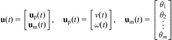
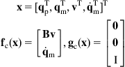
Here, the control of the five degrees of freedom MM studied in Section 10.3.3 will be considered [22]. We use the reduced dynamic model of Eq. (10.24) with parameters given by Eqs. (10.32)–(10.34). The vector ![]() of generalized variables is:
of generalized variables is:
![]() (10.44a)
(10.44a)
and the vector ![]() is:
is:
![]() (10.44b)
(10.44b)
To convert ![]() to the Cartesian coordinates velocity vector:
to the Cartesian coordinates velocity vector:
![]() (10.44c)
(10.44c)
we use the Jacobian relation (10.30a) and (10.30b).
![]() (10.44d)
(10.44d)
where the ![]() Jacobian matrix
Jacobian matrix ![]() is invertible. Differentiating Eq. (10.44d) we get:
is invertible. Differentiating Eq. (10.44d) we get:
![]()
which, if solved for ![]() , gives:
, gives:
![]() (10.45)
(10.45)
Now, introducing Eq. (10.45) into Eq. (10.24), and premultiplying by ![]() gives the model:
gives the model:
![]() (10.46)
(10.46)
where:
 (10.47)
If the desired path for ![]() is
is ![]() , and the error is defined as
, and the error is defined as ![]() , we select as usual the computed-torque law:
, we select as usual the computed-torque law:
![]() (10.48)
(10.48)
Introducing Eq. (10.48) into Eq. (10.46), under the assumption that the robot parameters are precisely known, gives:
![]() (10.49a)
(10.49a)
Now, we can use the linear feedback control law:
![]() (10.49b)
(10.49b)
In this case, the dynamics of the closed-loop error system is described by:
![]()
Therefore, selecting properly ![]() and
and ![]() we can get the desired performance specifications.
we can get the desired performance specifications.
10.4.2 Sliding-Mode Control of Omnidirectional MM
We work with the dynamic model of the MM, given by Eq. (10.42) which due to the omnidirectionality of the platform does not involve any nonholonomic constraint [8,11]. Applying computed-torque control:
![]() (10.50a)
(10.50a)
we arrive, as usual, to the linear dynamic system:
![]() (10.50b)
(10.50b)
![]() (10.50c)
(10.50c)
that leads to an asymptotically stable error dynamics.
If ![]() and
and ![]() are subject to uncertainties, and we know only their approximations
are subject to uncertainties, and we know only their approximations ![]() , then the computed-torque controller is:
, then the computed-torque controller is:
![]() (10.51a)
(10.51a)
and the system dynamics is given by:
![]() (10.51b)
(10.51b)
In this case, some appropriate robust control technique must be used. A convenient controller is the sliding-mode controller described in Section 7.2.2. This controller involves a nominal term (based on the computed-torque control law), and an additional term that faces the imprecision of the dynamic model.
The sliding condition for a multiple-input multiple-output system is a generalization of Eq. (7.14):
![]() (10.52a)
(10.52a)
with:
![]() (10.52b)
(10.52b)
where ![]() and
and ![]() is a Hurwitz (stable) matrix. The condition (10.52a) guarantees that the trajectories point towards the surface
is a Hurwitz (stable) matrix. The condition (10.52a) guarantees that the trajectories point towards the surface ![]() for all
for all ![]() . This can be shown by choosing a Lyapunov function of the form:
. This can be shown by choosing a Lyapunov function of the form:
![]()
where ![]() is the inertia matrix of the MM. Differentiating
is the inertia matrix of the MM. Differentiating ![]() we get:
we get:
![]() (10.53a)
(10.53a)
The control law is now defined as:
![]() (10.53b)
(10.53b)
where ![]() is a vector with components
is a vector with components ![]() . Furthermore, the
. Furthermore, the ![]() term is the control law part which could make
term is the control law part which could make ![]() , if there is no dynamic imprecision inside the estimated dynamic model, that is, according to Eq. (10.53a):
, if there is no dynamic imprecision inside the estimated dynamic model, that is, according to Eq. (10.53a):
![]()
where ![]() and
and ![]() are the available estimates of
are the available estimates of ![]() and
and ![]() . Now, calling
. Now, calling ![]() and
and ![]() the real matrices of the robot, we define the matrices:
the real matrices of the robot, we define the matrices:
![]()
as the bounds on the modeling errors. Then, it is possible to choose the components ![]() of the vector
of the vector ![]() such that:
such that:
![]() (10.54a)
(10.54a)
If this control mode is used, the condition:
![]() (10.54b)
(10.54b)
is verified to hold. This means that the sliding surface ![]() is reached in a finite time, and that once on the surface, the trajectories remain on the surface and, therefore, tend to
is reached in a finite time, and that once on the surface, the trajectories remain on the surface and, therefore, tend to ![]() exponentially.
exponentially.
Example 10.2
The end-effector of a five degrees of freedom planar MM is dragged by a human operator to follow a desired trajectory. The problem is:
(a) To derive a nonlinear controller that drives the mobile platform such that the end-effector follows this trajectory with a desired (preferred) manipulator configuration.
(b) To extend the method of (a) and find a state controller that achieves the trajectory tracking by completely compensating the platform–manipulator dynamic interaction.
Solution
(a) Clearly, the MM must track the desired trajectory with the manipulator fixed at the desired configuration which here is selected as the one that maximizes the manipulator’s manipulability measure (see Section 10.2.4.3):
The optimal configurations of the manipulator for which w is maximum are ![]() for any
for any ![]() and
and ![]() . Here we choose the desired angles
. Here we choose the desired angles ![]() and
and ![]() as shown in Figure 10.11A. If
as shown in Figure 10.11A. If ![]() the choice of
the choice of ![]() implies that the end-effector is located on a line parallel to the WMR axis which passes through the point
implies that the end-effector is located on a line parallel to the WMR axis which passes through the point ![]() .
.
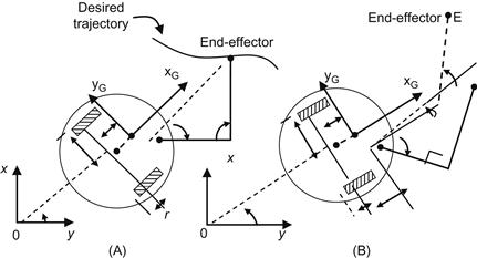
Figure 10.11 (A) The MM at the desired manipulator configuration ![]() and
and ![]() . The point
. The point ![]() is the COG of the platform with world coordinates
is the COG of the platform with world coordinates ![]() and
and ![]() . The world coordinates of the manipulator base point
. The world coordinates of the manipulator base point ![]() are
are ![]() and
and ![]() . (B) While the MM is moving to achieve trajectory tracking, the platform moves to bring the manipulator into the preferred configuration.
. (B) While the MM is moving to achieve trajectory tracking, the platform moves to bring the manipulator into the preferred configuration.
The coordinates ![]() (in the platform coordinate frame) of the manipulator end-effector at the desired (optimal) configuration are constant, being equal to:
(in the platform coordinate frame) of the manipulator end-effector at the desired (optimal) configuration are constant, being equal to:
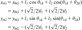
where ![]() and
and ![]() are the coordinates of the manipulator base
are the coordinates of the manipulator base ![]() in the platform coordinate frame
in the platform coordinate frame ![]() . It is remarked that any trajectory tracking error will result in getting the manipulator out of the desired configuration, thus reducing the value of the manipulability measure. We will apply the affine-systems methodology of Section 6.3.2 [23,24].
. It is remarked that any trajectory tracking error will result in getting the manipulator out of the desired configuration, thus reducing the value of the manipulability measure. We will apply the affine-systems methodology of Section 6.3.2 [23,24].
Since the manipulator is kept at the desired configuration, its dynamics is ignored. Therefore, we need only the dynamic model of the platform which in reduced form (with the nonholonomic constraint eliminated) has the affine state-space form of Eqs. (6.43a) and (6.43b):
where ![]() and
and ![]() are given by Eq. (6.41b) and:
are given by Eq. (6.41b) and:
Applying the computed-torque-like controller given by Eq. (6.44a):
![]()
where ![]() is a new control vector, the above model takes the form (6.45a)–(6.45c):
is a new control vector, the above model takes the form (6.45a)–(6.45c):
![]()
where:

We have seen in Section 6.3.2 that if the output components ![]() and
and ![]() are taken to be the coordinates of the wheels’ axis midpoint
are taken to be the coordinates of the wheels’ axis midpoint ![]() , the above model can be input–output linearizable (and decoupled) by using a dynamic nonlinear state-feedback controller, but it cannot be linearized by any static state-feedback controller. However, as explained in Example 6.8 it is possible to decouple the inputs and outputs using a static feedback controller if
, the above model can be input–output linearizable (and decoupled) by using a dynamic nonlinear state-feedback controller, but it cannot be linearized by any static state-feedback controller. However, as explained in Example 6.8 it is possible to decouple the inputs and outputs using a static feedback controller if ![]() and
and ![]() are the coordinates
are the coordinates ![]() of a reference point
of a reference point ![]() in front of the vehicle. To find the general conditions under which a differential-drive WMR can be input–output decoupled by static state-feedback control, we assume that the output vector components
in front of the vehicle. To find the general conditions under which a differential-drive WMR can be input–output decoupled by static state-feedback control, we assume that the output vector components ![]() and
and ![]() are the world coordinates
are the world coordinates ![]() and
and ![]() of an arbitrary reference point, that is:
of an arbitrary reference point, that is:
![]()
We now express ![]() and
and ![]() in the platform’s coordinate frame with origin at the platform COG
in the platform’s coordinate frame with origin at the platform COG ![]() . The result is:
. The result is:
![]()
where ![]() and
and ![]() are the coordinates of the reference point in the platform coordinate frame.
are the coordinates of the reference point in the platform coordinate frame.
Working as in Example 6.8 we find, via successive differentiation of ![]() , the dynamic model of
, the dynamic model of ![]() , namely:
, namely:
![]()
where ![]() is the matrix:
is the matrix:
![]()
with ![]() :
:

The determinant of ![]() is found to be:
is found to be:
![]()
which is different than zero if ![]() , that is, if the reference point is not a point of the WMR wheel axis. Therefore, if
, that is, if the reference point is not a point of the WMR wheel axis. Therefore, if ![]() , the matrix
, the matrix ![]() is nonsingular (i.e., it is a decoupling matrix) and can be inverted.2 As a result, choosing the state-feedback control law:
is nonsingular (i.e., it is a decoupling matrix) and can be inverted.2 As a result, choosing the state-feedback control law:
![]()
where ![]() , and
, and ![]() is the new control input vector:
is the new control input vector:
![]()
we get the decoupled system ![]() .
.
The fact that for decouplability the reference point must not lie on the WMR wheel axis is due to the nonholonomicity property which implies that a point on the wheel axis has instantaneously one degree of freedom, whereas all other points have instantaneously two degrees of freedom.
On the basis of the above, it follows that the overall static feedback controller that leads to a linear input–output decoupled system consists of the computed control-like part:
![]() (10.55a)
(10.55a)
and the decoupling part:
![]() (10.55b)
(10.55b)
with the result being ![]() , that is:
, that is:
![]() (10.55c)
(10.55c)
Now, the asymptotic tracking of the desired trajectory ![]() can be achieved by a linear PD controller as usual.
can be achieved by a linear PD controller as usual.
(b) In this case, we have to drive the MM at the desired trajectory and at the same time achieve the desired manipulator configuration. Therefore, we need the dynamic models of both the platform and the manipulator, which in combined reduced (unconstrained) form are given by Eq. (10.24):
![]()
where ![]() are given by the combination of the respective terms of the platform and manipulator, and:
are given by the combination of the respective terms of the platform and manipulator, and:
![]()
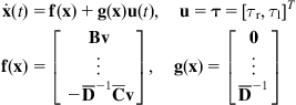
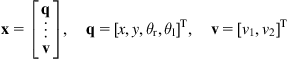
This model can be written in the state-space affine form:
![]()
where:
Here, we have four inputs, ![]() and so we can have input–output decoupling of up to four outputs. Therefore, we will select four outputs:
and so we can have input–output decoupling of up to four outputs. Therefore, we will select four outputs: ![]() . The manipulator end-effector cannot track the desired trajectory alone without the help of the mobile platform, because it may be overstretched reaching the boundary of its workspace. Therefore, while the manipulator is moving to track as much as possible the desired trajectory, the mobile platform should be controlled such that to bring the manipulator into the preferred configuration.
. The manipulator end-effector cannot track the desired trajectory alone without the help of the mobile platform, because it may be overstretched reaching the boundary of its workspace. Therefore, while the manipulator is moving to track as much as possible the desired trajectory, the mobile platform should be controlled such that to bring the manipulator into the preferred configuration.
The first two components of the output vector ![]() are selected to be the coordinates
are selected to be the coordinates ![]() of the point E in the platform coordinate frame (see Figure 10.11B), that is:
of the point E in the platform coordinate frame (see Figure 10.11B), that is:
![]()
To assure that the platform controller moves the platform so as to bring always the manipulator to the desired configuration, we choose the other two output components as:
![]()
which are the coordinates of the reference point R of Figure 10.11 in the world coordinate frame. Clearly, the desired values ![]() and
and ![]() of
of ![]() and
and ![]() must be set to the actual location of the end-effector position E such that to bring R to E, that is, the manipulator configuration into the preferred one.
must be set to the actual location of the end-effector position E such that to bring R to E, that is, the manipulator configuration into the preferred one.
Thus, the overall output vector ![]() is:
is:

From this point, the controller design proceeds as before. Differentiating twice the output ![]() we get:
we get:
![]()
where ![]() , and:
, and:

Therefore, selecting ![]() as:
as:
![]()
we get the linear decoupled system:
![]()
which can be controlled by a diagonal PD state-feedback controller as usual with given desired natural frequency ![]() and damping ratio
and damping ratio ![]() . As an exercise, the reader is advised to solve the problem by taking into consideration the WMR maneuverability. The above controllers for the problems (a) and (b) were tested by simulation in Refs. [23,24] showing very satisfactory performance (see Section 13.9.2). It is noted that the tracking control problem studied in Section 10.4.1 is a special case of the present problem (b) in which the maximum (or other desired) manipulability measure condition is relaxed.
. As an exercise, the reader is advised to solve the problem by taking into consideration the WMR maneuverability. The above controllers for the problems (a) and (b) were tested by simulation in Refs. [23,24] showing very satisfactory performance (see Section 13.9.2). It is noted that the tracking control problem studied in Section 10.4.1 is a special case of the present problem (b) in which the maximum (or other desired) manipulability measure condition is relaxed.
2Note that the computed-torque control technique applied in Section 5.5 for the reference point C that does not belong to the common wheel axis (i.e., b≠0) is a special case of this general input–output linearizing and decoupling static feedback controller.
10.5 Vision-Based Control of MMs
10.5.1 General Issues
As described in Section 9.4, the image-based visual control uses the image Jacobian (or interaction) matrix. Actually, the inverse or generalized inverse of the Jacobian matrix or its generalized transpose is used, in order to determine the screw (or velocity twist) ![]() of the end-effector which assures the achievement of a desired task. In MMs where the platform is omnidirectional (and does not involve any nonholonomic constraint), the method discussed in Section 9.4 is directly applicable. However, if the MM platform is nonholonomic, special care is required for both determining and using the corresponding image Jacobian matrix. This can be done by combining the results of Sections 9.2, 9.4, and 10.3.
of the end-effector which assures the achievement of a desired task. In MMs where the platform is omnidirectional (and does not involve any nonholonomic constraint), the method discussed in Section 9.4 is directly applicable. However, if the MM platform is nonholonomic, special care is required for both determining and using the corresponding image Jacobian matrix. This can be done by combining the results of Sections 9.2, 9.4, and 10.3.
The Jacobian matrix is defined by Eq. (9.11) and relates the end-effector screw:
![]() (10.56a)
(10.56a)
with the feature vector rate of change:
![]() (10.56b)
(10.56b)
that is:
![]() (10.56c)
(10.56c)
The relation of ![]() to
to ![]() , where
, where ![]() is the position vector
is the position vector ![]() rigidly attached to the end-effector, is given by Eq. (9.4a):
rigidly attached to the end-effector, is given by Eq. (9.4a):
![]() (10.57)
(10.57)
where ![]() is the skew symmetric matrix of Eq. (9.4b). The matrix
is the skew symmetric matrix of Eq. (9.4b). The matrix ![]() is the robot Jacobian part. The relation of
is the robot Jacobian part. The relation of ![]() to
to ![]() is given by Eq. (9.13a):
is given by Eq. (9.13a):
![]() (10.58a)
(10.58a)
where:
![]() (10.58b)
(10.58b)
The matrix ![]() is the camera interaction part. Combining Eqs. (10.57) and (10.58a) we get the expression of
is the camera interaction part. Combining Eqs. (10.57) and (10.58a) we get the expression of ![]() , namely,
, namely,
![]() (10.59)
(10.59)
as given in Eq. (9.15) for the case of two image plane features ![]() and
and ![]() .
.
Now, we will examine the case where the task features are the components of the vector:
![]()
In this case, the camera interaction part ![]() , in Eq. (10.58b), is given by:
, in Eq. (10.58b), is given by:
 (10.60a)
for ![]() . Therefore, the overall Jacobian matrix
. Therefore, the overall Jacobian matrix ![]() is given by:
is given by:
 (10.60b)
The control of the MM needs the control of the platform and the manipulator mounted on it. Two ways to do this are the following:
1. Control the platform and the arm separately, and then treat the existing coupling between them.
2. Control the platform and the arm jointly with the coupling kinematics and dynamics included in the overall model used (full-state model).
Example 10.3
Outline a method for MM visual-based point stabilization, taking into consideration the coupling that exists between the platform and the manipulator.
Solution
We will consider the problem of stabilizing an MM in a desired configuration using measurements of the manipulator (arm) joint positions and the measures (feature measurements) provided by an onboard camera mounted on the end-effector. This problem involves the following requirements:
1. To reduce asymptotically to zero the feature errors provided by the camera measurements.
2. To move the platform such that, during the arm control for reducing the feature errors, to maintain the manipulator in the nonsingular configuration space.
3. To steer the platform such that to have the manipulator to the desired configuration, while the arm is controlled to keep constant the camera measures.
These requirements can be satisfied using a hybrid control scheme that merges a feedback and an open-loop control strategy as follows [18].
Feedback Control
The feedback control ![]() drives the camera measurement errors asymptotically to zero, and, at the same time, maintains the manipulator far from singularities. If
drives the camera measurement errors asymptotically to zero, and, at the same time, maintains the manipulator far from singularities. If ![]() is the error between the actual and desired image features, then
is the error between the actual and desired image features, then ![]() , and the manipulator position
, and the manipulator position ![]() must be such that
must be such that ![]() as
as ![]() , asymptotically, that is, such that:
, asymptotically, that is, such that:
![]() (10.61)
(10.61)
where ![]() is a matrix gain determining the rate of convergence.
is a matrix gain determining the rate of convergence.
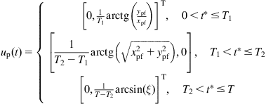
The kinematic model of the MM from the input velocities to the features’ rate of variation ![]() has the form of Eq. (10.21a), that is:
has the form of Eq. (10.21a), that is:
![]() (10.62)
(10.62)
where ![]() is the vector of the manipulator joint positions,
is the vector of the manipulator joint positions, ![]() is the platform position/orientation vector,
is the platform position/orientation vector, ![]() and
and ![]() are the platform and manipulator image Jacobian matrices, respectively, and
are the platform and manipulator image Jacobian matrices, respectively, and ![]() is the platform control vector (linear velocity,
is the platform control vector (linear velocity, ![]() , and angular velocity,
, and angular velocity, ![]() ). The image Jacobian matrices
). The image Jacobian matrices ![]() and
and ![]() consist of the robot part and camera part as shown in Eq. (10.59). Note that if we use three landmark points the camera part is a
consist of the robot part and camera part as shown in Eq. (10.59). Note that if we use three landmark points the camera part is a ![]() matrix, and if these landmarks are not aligned the matrix is nonsingular (see Eqs. (10.60a), (10.60b), and (9.15)).
matrix, and if these landmarks are not aligned the matrix is nonsingular (see Eqs. (10.60a), (10.60b), and (9.15)).
To get Eq. (10.61), ![]() in Eq. (10.62) must be selected as:
in Eq. (10.62) must be selected as:
![]() (10.63)
(10.63)
Now if the desired position of the manipulator is ![]() , we get
, we get ![]() and
and ![]() . Therefore, selecting the platform control vector
. Therefore, selecting the platform control vector ![]() as:
as:
![]() (10.64)
(10.64)
we obtain:
![]() (10.65)
(10.65)
where the gain ![]() must be suitably selected such that to have the desired rate of convergence to zero.
must be suitably selected such that to have the desired rate of convergence to zero.
To keep the arm far from singular configurations, the above two controllers must be suitably coordinated. To this end, ![]() in Eq. (10.64) is modified as:
in Eq. (10.64) is modified as:
![]() (10.66)
(10.66)
where ![]() is a threshold ensuring the avoidance of singular configurations, and
is a threshold ensuring the avoidance of singular configurations, and ![]() is a suitable strictly decreasing function such as:
is a suitable strictly decreasing function such as:
![]() (10.67)
(10.67)
with proper coefficients ![]() and
and ![]() . Indeed, for manipulator configurations far from the desired configuration (where also singular configurations may occur), we have
. Indeed, for manipulator configurations far from the desired configuration (where also singular configurations may occur), we have ![]() and
and ![]() . Therefore, the manipulator is forced to compensate only the motion of the platform which is controlled to reduce
. Therefore, the manipulator is forced to compensate only the motion of the platform which is controlled to reduce ![]() according to Eq. (10.64).
according to Eq. (10.64).
Open-Loop Control
The open-loop control ![]() is to steer the platform so as to have the manipulator to the desired configuration
is to steer the platform so as to have the manipulator to the desired configuration ![]() , while the arm is controlled to maintain constant the camera measures.
, while the arm is controlled to maintain constant the camera measures.
The hybrid control scheme is as follows:
![]() (10.68)
(10.68)
where ![]() is a selected time period, and
is a selected time period, and ![]() Given an initial configuration
Given an initial configuration ![]() , the open-loop control must assure that
, the open-loop control must assure that ![]() , and
, and ![]() belongs to the nonsingular configuration space for all
belongs to the nonsingular configuration space for all ![]() , where
, where ![]() and
and ![]() . Setting
. Setting ![]() in Eq. (10.63) (i.e., no feature feedback control) we get:
in Eq. (10.63) (i.e., no feature feedback control) we get:
![]() (10.69)
(10.69)
Now, for a given ![]() , we have:
, we have:
![]() (10.70)
(10.70)
and so the joint trajectory is fully determined by ![]() and
and ![]() . Therefore, as long as the arm is controlled using Eq. (10.69), the open-loop control problem is to compute an open-loop platform control
. Therefore, as long as the arm is controlled using Eq. (10.69), the open-loop control problem is to compute an open-loop platform control ![]() such that
such that ![]() , and
, and ![]() is a nonsingular configuration for all
is a nonsingular configuration for all ![]() . Actually, many such control sequences can be found. For the planar case, it can be verified that the sequence:
. Actually, many such control sequences can be found. For the planar case, it can be verified that the sequence:
 (10.71)
does the job. Here, ![]() is the platform final configuration,
is the platform final configuration, ![]() , and:
, and:
![]()
with the assumption that the platform coordinate frame coincides with the world coordinate frame [18].
10.5.2 Full-State MM Visual Control
The vision-based control of mobile platforms was studied in Section 9.5, where several representative problems (pose stabilizing control, wall following control, etc.) were considered. Here we will consider the pose stabilizing control of MMs combining the platform pose and manipulator/camera pose control [3,14]. Actually, the results of Section 9.5.1 concern the case of stabilizing the platform’s pose ![]() and the camera’s pose
and the camera’s pose ![]() . The camera pose control can be regarded as the stabilizing pose control of a one-link manipulator (using the notation
. The camera pose control can be regarded as the stabilizing pose control of a one-link manipulator (using the notation ![]() ). Therefore, the vision-based control of a general MM can be derived by direct extension of the controller derived in Section 9.5.1. This controller is given by Eqs. (9.49a), (9.49b), (9.50a), and (9.50b), and stabilizes to zero the total pose vector:
). Therefore, the vision-based control of a general MM can be derived by direct extension of the controller derived in Section 9.5.1. This controller is given by Eqs. (9.49a), (9.49b), (9.50a), and (9.50b), and stabilizes to zero the total pose vector:
![]()
on the basis of feature measurements:
![]()
of three nonaligned target feature points ![]() and
and ![]() , provided by an onboard camera, and a sensor measuring
, provided by an onboard camera, and a sensor measuring ![]() (see Figure 9.4). This controller employs the image Jacobian relation (9.25a) and (9.25b):
(see Figure 9.4). This controller employs the image Jacobian relation (9.25a) and (9.25b):
![]()
where ![]() and
and ![]() are given by Eqs. (9.21) and (9.24b), respectively.
are given by Eqs. (9.21) and (9.24b), respectively.
Using three feature points as in Figure 9.4, the camera part ![]() of the Jacobian
of the Jacobian ![]() has the same form as in Eq. (9.21). But the robot part
has the same form as in Eq. (9.21). But the robot part ![]() of the image Jacobian is different depending on the number and type of the manipulator links.
of the image Jacobian is different depending on the number and type of the manipulator links.
For example, if we consider the five-link MM of Figure 10.8, the Jacobian matrix of the overall system (including the coupling between the platform and the manipulator) is given by Eqs. (10.30a) and (10.30b), where the wheel motor velocities ![]() and
and ![]() are equivalently used as controls instead of
are equivalently used as controls instead of ![]() and
and ![]() . Now, the controller design proceeds in the usual way as described in Sections 9.3 and 9.4 for both cases of position-based and image-based control.
. Now, the controller design proceeds in the usual way as described in Sections 9.3 and 9.4 for both cases of position-based and image-based control.
Example 10.4
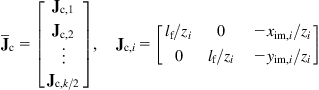
We consider a five degrees of freedom MM consisting of a four degrees of freedom articulated robotic manipulator, a one degree of freedom linear slide, a fixed camera, and a stationary spherical mirror as shown in Figure 10.12. Assuming that two fictitious landmarks are mounted on the end-effector, the problem is to derive an appropriate image Jacobian that can be used for 3D visual servoing of the MM.
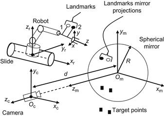
Figure 10.12 Structure of MM/spherical catadioptric vision system. The optical axis of the camera passes through the center ![]() .
.
Solution
The system has the structure of Figure 9.3B with the following coordinate frames:
The mirror frame is mapped to the camera frame by the homogenous transformation:
 (10.72)
where d is the distance of the mirror and camera. Similarly, the camera frame can be transformed to the robot frame by ![]() . The relationship between the landmarks
. The relationship between the landmarks ![]() and their mirror projections (reflections)
and their mirror projections (reflections) ![]() and
and ![]() represented in the spherical mirror frame is found using the spherical convex mirror reflection rule as [25,26]:
represented in the spherical mirror frame is found using the spherical convex mirror reflection rule as [25,26]:
![]() (10.73)
(10.73)
where R is the spherical mirror radius. Using Eqs. (10.72) and (10.73) one finds that the transformation from the landmarks and their mirror reflections in ![]() to those in the camera frame
to those in the camera frame ![]() are:
are:
![]() (10.74)
(10.74)
from which we obtain that the landmarks’ coordinates to its mirror reflection, represented in the camera frame, are given by (compare with the geometry of Figure 9.22):
![]() (10.75)
(10.75)
Differentiating Eq. (10.75), we find the transformation ![]() of the velocity screw of the landmarks to their mirror reflections, represented in the camera frame, namely:
of the velocity screw of the landmarks to their mirror reflections, represented in the camera frame, namely:
![]() (10.76)
(10.76)
where:

with ![]() .
.
As we know (see Figures 9.21 and 9.22) in a spherical catadioptric vision system, the camera is a typical perspective camera which, in general, is described by:
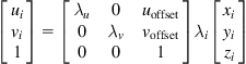 (10.77)
with ![]() being the image coordinates in the 2D image plane,
being the image coordinates in the 2D image plane, ![]() where
where ![]() is the camera focal length,
is the camera focal length, ![]() and
and ![]() are scaling factors that correspond to the effective pixels’ size in the horizontal and vertical directions, and
are scaling factors that correspond to the effective pixels’ size in the horizontal and vertical directions, and ![]() are offset parameters that represent the principal point of the image in the pixel frame (typically at or near the image center).
are offset parameters that represent the principal point of the image in the pixel frame (typically at or near the image center).
Now, let ![]() and
and ![]() be the 2D image plane coordinates of the landmarks #1 and #2 mounted on the end-effector. Similarly, let
be the 2D image plane coordinates of the landmarks #1 and #2 mounted on the end-effector. Similarly, let ![]() and
and ![]() be the mirror reflections of the landmarks on the image plane (Figure 10.13) [25]. Thus, actually we have eight features:
be the mirror reflections of the landmarks on the image plane (Figure 10.13) [25]. Thus, actually we have eight features:
![]()

By bringing these features to their desired values in the image plane where:
![]()
(simultaneously) we can have 3D visual control of the end-effector.
Since the landmarks on the end-effector are considered as geometric points, they do not possess any roll motion. Therefore, in the present case, the above eight features can be reduced to five features, still allowing 3D visual servoing. These five features can be found using any possible morphology. Referring to Figure 10.13 one can choose the following five features: ![]() and
and ![]() where
where ![]() and
and ![]() are the distances between the landmarks and their images,
are the distances between the landmarks and their images, ![]() and
and ![]() are the distances between the middle points of the line segments.
are the distances between the middle points of the line segments.
![]() and
and ![]() , and
, and ![]() is the distance between the one-thirds of the above line segments [25,26]. From the geometry of Figure 10.13 we find that:
is the distance between the one-thirds of the above line segments [25,26]. From the geometry of Figure 10.13 we find that:

where ![]() and
and ![]() are the 2D image coordinates of the midpoint of the line segment connecting the desired positions of the landmarks and their images (reflections), respectively, and
are the 2D image coordinates of the midpoint of the line segment connecting the desired positions of the landmarks and their images (reflections), respectively, and ![]() represent the 2D image coordinates of the one-third of the line segment that connects the desired position of landmark #1 and its reflection, projected onto the 2D image plane. Clearly:
represent the 2D image coordinates of the one-third of the line segment that connects the desired position of landmark #1 and its reflection, projected onto the 2D image plane. Clearly:
 (10.78)
This means that the values of the features ![]() and
and ![]() are invariant in terms of the image information obtained on the real landmarks or their reflections. This is not so for the feature
are invariant in terms of the image information obtained on the real landmarks or their reflections. This is not so for the feature ![]() , and so one can use
, and so one can use ![]() to distinguish the landmarks from their projections on the image plane. Indeed it was shown in Ref. [27] that with the above 5D feature vector:
to distinguish the landmarks from their projections on the image plane. Indeed it was shown in Ref. [27] that with the above 5D feature vector:
![]()
the mirror reflection of a landmark projected onto the image plane will always remain closer to the center of the image plane than from the landmark. Thus, a real landmark can be distinguished from its mirror reflection without the need of any image tracking. It is noted that special care has to be taken if a real landmark and its mirror reflection are seen to be the same on the image plane. In this case, the singularity can be avoided by moving the robot around the singular configuration.
We now have to study the motion of the landmarks in the 3D space. To this end, we consider as end-effector (tip) point the midpoint between the landmarks in the robot’s base coordinate frame. The relevant geometry is shown in Figure 10.14 [25].

In Figure 10.14, let us assume that ![]() is the midpoint between the landmarks
is the midpoint between the landmarks ![]() and
and ![]() where the upper index r denotes position coordinate in the robot coordinate frame. Here,
where the upper index r denotes position coordinate in the robot coordinate frame. Here, ![]() is the angle between the x-axis of the robot coordinate frame and the projection on the xy-plane of the line segment between the points
is the angle between the x-axis of the robot coordinate frame and the projection on the xy-plane of the line segment between the points ![]() and
and ![]() .
.
The angle ![]() is the angle between the line segment defined by the above two points and the xy-plane of the robot coordinate frame.
is the angle between the line segment defined by the above two points and the xy-plane of the robot coordinate frame.
Denoting by D the distance between the landmarks in the world coordinate frame we find that:
 (10.79)
The image Jacobian matrix which relates the velocity screw:
![]() (10.80)
(10.80)
of the landmark midpoint coordinate frame (with origin at ![]() ) and the image feature rate vector:
) and the image feature rate vector:
![]() (10.81)
(10.81)
can be found, as usual, by differentiating Eqs. (10.78) and (10.79), namely:
![]() (10.82)
(10.82)
Now, defining the feature error ![]() , the control law that assures asymptotic convergence of
, the control law that assures asymptotic convergence of ![]() to zero is the resolved-rate control law given by Eq. (9.34):
to zero is the resolved-rate control law given by Eq. (9.34):
![]() (10.83)
(10.83)
where K is a constant positive definite gain matrix (usually diagonal). Of course, if ![]() is not exactly known we can use in Eq. (10.83) an estimate
is not exactly known we can use in Eq. (10.83) an estimate ![]() which can be found as explained in Section 9.4.3 using the estimates of the camera-intrinsic and -extrinsic parameters. Here, the intrinsic parameters include the two scaling factors
which can be found as explained in Section 9.4.3 using the estimates of the camera-intrinsic and -extrinsic parameters. Here, the intrinsic parameters include the two scaling factors ![]() and the two offset terms
and the two offset terms ![]() and
and ![]() . The extrinsic parameter is the distance d of the camera frame from the mirror’s center. Therefore, the vector
. The extrinsic parameter is the distance d of the camera frame from the mirror’s center. Therefore, the vector ![]() that has to be estimated is:
that has to be estimated is:
![]()
while the measurement vector ![]() is:
is:
![]()
References
1. Padois V, Fourquet JY, Chiron P. Kinematic and dynamic model-based control of wheeled mobile manipulators: a unified framework for reactive approaches. Robotica. 2007;25(2):157–173.
2. Seelinger M, Yoder JD, Baumgartner ET, Skaar BR. High-precision visual control of mobile manipulators. IEEE Trans Robot Autom. 2002;18(6):957–965.
3. Tzafestas CS, Tzafestas SG. Full-state modeling, motion planning and control of mobile manipulators. Stud Inform Control. 2001;10(2):109–127.
4. Kumara P, Abeygunawardhana W, Murakami T. Control of two-wheel mobile manipulator on a rough terrain using reaction torque observer feedback. J Autom Mobile Robot Intell Syst. 2010;4(1):56–67.
5. Chung JH, Velinsky SA. Robust interaction control of a mobile manipulator: dynamic model based coordination. J Intell Robot Syst. 1999;26(1):47–63.
6. Li Z, Chen W, Liu H. Robust control of wheeled mobile manipulators using hybrid joints. Int J Adv Rob Syst. 2008;5(1):83–90.
7. Yamamoto Y, Yun X. Effect of the dynamic interaction on coordinated control of mobile manipulators. IEEE Trans Rob Autom. 1996;12(5):816–824.
8. Tzafestas SG, Melfi A, Krikochoritis T. Omnidirectional mobile manipulator modeling and control: analysis and simulation. Syst Anal Model Control. 2001;40:329–364.
9. Mazur A, Szakiel D. On path following control of non-holonomic mobile manipulators. Int J Appl Math Comput Sci. 2009;19(4):561–574.
10. Meghadari A, Durali M, Naderi D. Investigating dynamic interaction between one d.o.f manipulator and vehicle of a mobile manipulator. J Intell Robot Syst. 2000;28:277–290.
11. Watanabe K, Sato K, Izumi K, Kunitake Y. Analysis and control for an omnidirectional mobile manipulator. J Intell Robot Syst. 2000;27(1–2):3–20.
12. De Luca A, Oriolo G, Giordano PR. Image-based visual servoing schemes for nonholonomic mobile manipulators. Robotica. 2007;25:131–145.
13. Burshka D, Hager G. Vision-based control of mobile robots. In: Proceedings of 2001 IEEE international conference robotics and automation. Seoul, Korea; May 21–26, 2001.
14. Tsakiris D, Samson C, Rives P. Vision-based time-varying stabilization of a mobile manipulator. In: Proceedings of fourth international conference on control, automation, robotics and vision (ICARCV’96). Westin Stanford, Singapore; December 3–6, 1996. p. 1–5.
15. Yu Q, Chen Ming I. A general approach to the dynamics of nonholonomic mobile manipulator systems. Trans ASME. 2002;124:512–521.
16. DeLuca A, Oriolo G, Giordano PR. Kinematic control of nonholonomic mobile manipulators in the presence of steering wheels. In: Proceedings of 2010 IEEE international conference on robotics and automation. Anchorage, AK; May 3–8, 2010. p. 1792–98.
17. Phuoc LM, Martinet P, Kim H, Lee S. Motion planning for nonholonomic mobile manipulator based visual servo under large platform movement errors at low velocity. In: Proceedings of 17th IFAC world congress. Seoul, Korea; July 6–11, 2008. p. 4312–17.
18. Gilioli M, Melchiori C. Coordinated mobile manipulator point-stabilization using visual-servoing techniques. In: Proceedings of IEEE/RSJ international conference on intelligent robots and systems. Lausanne, CH; 2002. p. 305–10.
19. Ma Y, Kosecha J, Sastry S. Vision guided navigation for nonholonomic mobile robot. IEEE Trans Robot Autom. 1999;15(3):521–536.
20. Zhang Y. Visual servoing of a 5-DOF mobile manipulator using an omnidirectional vision system. Technical Report RML-3-2, University of Regina, 2006.
21. Bayle B, Fourquet JY, Renaud M. Manipulability analysis for mobile manipulators. In: Proceedings of 2001 IEEE international conference on robotics and automation. Seoul, Korea; May 21–26, 2001. p. 1251–56.
22. Papadopoulos E, Poulakakis J. Trajectory planning and control for mobile manipulator systems. In: Proceedings of eighth IEEE Mediterranean conference on control and automation. Patras, Greece; July 17–19, 2000.
23. Yamamoto Y, Yun X. Coordinating locomotion and manipulation of a mobile manipulator. In: Proceedings of 31st IEEE conference on decision and control. Tucson, AZ; December, 1992. p. 2643–48.
24. Yamamoto Y, Yun X. Modeling and compensation of the dynamic interaction of a mobile manipulator. In: Proceedings of IEEE conference on robotics and automation. San Diego, CA; May 8–13, 1994. p. 2187–92.
25. Zhang Y, Mehrandezh M. Visual servoing of a 5-DOF mobile manipulator using a panoramic vision system. In: Proceedings of 2007 Canadian conference on electrical and computer engineering. Vancouver, BC, Canada; April 22–26, 2007. p. 453–56.
26. Zhang Y, Mehrandezh M. Visual servoing of a 5-DOF mobile manipulator using a catadioptric vision system. In: Proceedings of SPIE, the international society for optical engineering; 2007. p. 6–17.
27. Zhang Y. Visual servoing of a 5-DOF mobile manipulator using panoramic vision system [M.Sc. thesis]. Regina, Canada, Faculty of Engineering, University of Regina, 2007.
1If there is friction ![]() in the motors of the joints (e.g.,
in the motors of the joints (e.g., ![]() friction coefficient), then
friction coefficient), then ![]() should be replaced by
should be replaced by ![]() .
.