
Mobile Robot Control I
The Lyapunov-Based Method
This chapter deals with the general problem of determining the forces and torques that must be developed by the robotic actuators in order for the robot to go at a desired position/posture, track a desired trajectory, and, in general, to perform some task with a desired quality of performance. The controllers to be presented in the chapter assume that the goal of the control and the robot dynamic parameters are precisely known, and if this goal (posture or path) is changing, the change is compatible with the environment, and risk free. The particular objectives of the chapter are (i) to provide a minimal set of general control concepts and methods that are used in robot control, (ii) to study the basic general robot controllers that are applicable to all types of robots, and (iii) to present a number of feedback controllers, designed using the Lyapunov-based control theory, for the differential drive, car-like, and omnidirectional mobile robots. These controllers refer to the problems of position (posture) tracking, trajectory tracking, parking, and leader following.
Keywords
Lyapunov stability; DC motor model; state feedback control; computed torque control; kinematic tracking control; dynamic tracking control; polar coordinate-based robot model; parking control; leader–follower control; kinematic controller; dynamic controller; omnidirectional robot control
5.1 Introduction
Robot control deals with the problem of determining the forces and torques that must be developed by the robotic actuators in order for the robot to go at a desired position, track a desired trajectory, and, in general, to perform some task with desired performance requirements. The solution to control problems in robotics (fixed and mobile) is more complicated than usual due to the inertial forces, coupling reaction forces, and gravity effects. The performance requirements concern both the transient period and the steady-state period. In well-structured and fixed environments, such as the factory, the environment can be arranged to match the capabilities of the robot. In these cases, it can be assured that the robot knows certainly the configuration of the environment, and people are protected from the robot’s operation. In such controlled environments, it is sufficient to employ some type of model-based control, but in uncertain and varying (uncontrolled) environments, the control algorithms must be more sophisticated involving some kind of intelligence. The techniques to be presented in this chapter assume that the goal of the control and the robot kinematic and dynamic parameters are precisely known, and if this goal (posture or path) is changing, the change is compatible with the environment, and risk free.
Specifically, the objectives of the chapter are as follows:
• To provide a minimal set of general control concepts and methods that are used in the control of robots
• To study the basic general robot controllers that are applicable to all types of robots
• To present a number of feedback controllers, designed using the Lyapunov-based control theory, for the differential drive, car-like, and omnidirectional mobile robots.
These controllers refer to the problems of position (posture) tracking, trajectory tracking, parking, and leader following. In all cases, the control design involves two stages, viz., kinematic control (where only the kinematic models are used), and dynamic control (where the robot dynamics and actuators are also taken into account).
5.2 Background Concepts
In this section, the following fundamental control concepts and techniques are briefly discussed:
Knowledge of these concepts is a basic prerequisite for the understanding of the material presented in the chapter. Full accounts are given in standard control textbooks [1].
5.2.1 State-Space Model
The state-space model of a control system is based on the concept of state vector ![]() , which is the minimum dimensionality Euclidean vector, with components called state variables, the knowledge of which at an initial time
, which is the minimum dimensionality Euclidean vector, with components called state variables, the knowledge of which at an initial time ![]() , together with the input vector
, together with the input vector ![]() , for
, for ![]() , determines completely the behavior of the system for any time
, determines completely the behavior of the system for any time ![]() . The dimension
. The dimension ![]() of the state vector specifies the system’s dimensionality.
of the state vector specifies the system’s dimensionality.
The above definition of the state means that the state of the system is determined by its initial value ![]() at
at ![]() and the input for
and the input for ![]() , and is independent of the state and the inputs for times previous to
, and is independent of the state and the inputs for times previous to ![]() .
.
It is noted that the state variables ![]() of an n-dimensional system may not necessarily be measurable physical quantities, although in practice, an effort is made to use as more as possible measurable variables, because the state feedback control laws need all of them.
of an n-dimensional system may not necessarily be measurable physical quantities, although in practice, an effort is made to use as more as possible measurable variables, because the state feedback control laws need all of them.
The expression of ![]() as a function of
as a function of ![]() , and
, and ![]() ,
, ![]() , that is,
, that is, ![]() , is called the system’s trajectory.
, is called the system’s trajectory.
The output ![]() of the system is a similar function of
of the system is a similar function of ![]() ,
, ![]() , and
, and ![]() , that is:
, that is:
![]()
The trajectories satisfy the transition property:
![]()
for all ![]() , where
, where ![]() .
.
In state-space model, the dynamic model of a nonlinear system (in continuous time) has the form:
![]() (5.1a)
(5.1a)
![]() (5.1b)
(5.1b)
where ![]() and
and ![]() are nonlinear vector functions of their arguments with proper dimensionality and the continuity and smoothness properties required in each case. The state vector
are nonlinear vector functions of their arguments with proper dimensionality and the continuity and smoothness properties required in each case. The state vector ![]() belongs to the state space
belongs to the state space ![]() , the input (control)
, the input (control) ![]() belongs to the input space
belongs to the input space ![]() , and the output
, and the output ![]() to the output space
to the output space ![]() , where
, where ![]() ,
, ![]() ,
, ![]() , and
, and ![]() is the n-dimensional Euclidean space.
is the n-dimensional Euclidean space.
If the vector functions ![]() and
and ![]() are linear, then the system is linear and is described by the model:
are linear, then the system is linear and is described by the model:
![]() (5.2a)
(5.2a)
![]() (5.2b)
(5.2b)
where ![]() ,
, ![]() ,
, ![]() ,
, ![]() may be time-invariant or time-varying matrices of proper dimensionality (in many cases,
may be time-invariant or time-varying matrices of proper dimensionality (in many cases, ![]() ). A linear state-space model with the following matrices,
). A linear state-space model with the following matrices, ![]() ,
, ![]() , and
, and ![]() (scalar), is called the controllable canonical model of the system that represents:
(scalar), is called the controllable canonical model of the system that represents:
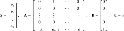 (5.3)
(5.3)
For a scalar output ![]() , a linear time-invariant system described by the nth-order differential equation:
, a linear time-invariant system described by the nth-order differential equation:
![]()
or transfer function:
![]() (5.4)
(5.4)
where ![]() is the complex frequency variable, can be modeled as in Eqs. (5.2a), (5.2b), and (5.3), if we define the state variables
is the complex frequency variable, can be modeled as in Eqs. (5.2a), (5.2b), and (5.3), if we define the state variables ![]() as:
as:
![]() (5.5)
(5.5)
Indeed, using Eq. (5.5) we get:
![]()
![]()
which gives the state-space model ((5.2a), (5.2b), and (5.3)) with:
![]() (5.6)
(5.6)
This model, also called phase variables canonical model, is very convenient for the pole-placement (or assignment) state feedback controller design.
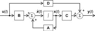
The block diagram representation of the general model (5.2a) and ((5.2b)) has the form shown in Figure 5.1.
Other state-space canonical models of the system (5.2a) and ((5.2b)) are the observable canonical form and the Jordan canonical form fully described in control textbooks. To convert a given model (5.2a) and ((5.2b)) to some canonical form, use is made of a proper nonsingular linear (similarity) transformation ![]() , where
, where ![]() is the new state vector.
is the new state vector.
Example 5.1
In this example, we derive the dynamic models (transfer function, state-space model) of the direct current (DC) electrical motor which is used in mobile robots to provide the torques that lead to the desired acceleration and velocity of them. DC motors are distinguished into motors controlled by the rotor (armature controlled), and motors controlled by the stator (field controlled). Both the motors will be considered.
Armature Controlled DC Motor
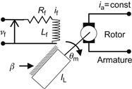
The rotor involves the armature and the commutator. A schematic of this motor is shown in Figure 5.2, where ![]() and
and ![]() are the resistance and inductance of the rotor,
are the resistance and inductance of the rotor, ![]() is the load moment of inertia, and
is the load moment of inertia, and ![]() is the linear friction coefficient.
is the linear friction coefficient.
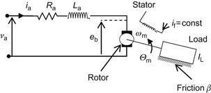
Figure 5.2 Schematic of the armature controlled DC motor (![]() =rotation angle,
=rotation angle, ![]() =motor angular speed,
=motor angular speed, ![]() =load moment of inertia).
=load moment of inertia).
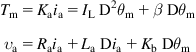
The mechanical torque is given by:
![]() (5.7)
(5.7)
where ![]() is the motor’s torque constant. The back electromotive force (emf)
is the motor’s torque constant. The back electromotive force (emf) ![]() which is subtracted from the input voltage
which is subtracted from the input voltage ![]() is proportional to
is proportional to ![]() , that is:
, that is:
![]() (5.8)
(5.8)
The characteristic curves of “![]() ” are obtained by plotting the following function:
” are obtained by plotting the following function:
![]()
and have the linear form shown in Figure 5.3.
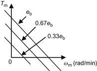
At the point where ![]() , the motor maintains a constant angular speed (assuming of course that no external disturbances affect the motor). The differential equation of the motor can be found using the following relations:
, the motor maintains a constant angular speed (assuming of course that no external disturbances affect the motor). The differential equation of the motor can be found using the following relations:
where ![]() ,
, ![]() is the moment of inertia of the load (plus the moment of inertia of the motor), and
is the moment of inertia of the load (plus the moment of inertia of the motor), and ![]() is the linear friction coefficient, and eliminating
is the linear friction coefficient, and eliminating ![]() . The result is:
. The result is:
![]()
where ![]()
![]()
![]()
![]()
![]() . If
. If ![]() is negligible, then
is negligible, then ![]() , and the above differential equation reduces to:
, and the above differential equation reduces to:
![]() (5.9)
(5.9)
where ![]() is as above, and
is as above, and ![]() . In practice, the model in Eq. (5.9) represents an adequate approximation of the motor dynamics. The controllable state-space canonical model of the motor is found from Eq. (5.9) using Eqs. (5.3) and (5.6), that is:
. In practice, the model in Eq. (5.9) represents an adequate approximation of the motor dynamics. The controllable state-space canonical model of the motor is found from Eq. (5.9) using Eqs. (5.3) and (5.6), that is:
![]() (5.10)
(5.10)
with ![]() and
and ![]() . A DC motor is shown in Figure 5.4A. Figure 5.4B shows DC motors of several sizes.
. A DC motor is shown in Figure 5.4A. Figure 5.4B shows DC motors of several sizes.

Figure 5.4 (A) A heavy-duty DC robot motor. (B) Several DC motors with embedded gear boxes. Source: http://www.goldmine-elec-products.com/prodinfo.asp?number=0; http://www.robojrr.tripod.com/motortech.htm.
Field Controlled DC motor
In this motor, the rotor’s current is kept constant (coming from a constant-current source), whereas the error is fed to the magnetic field of the stator via a phase-sensitive amplifier (Figure 5.5). The characteristic curves ![]() show that when
show that when ![]() is not excessively large, the mechanical torque
is not excessively large, the mechanical torque ![]() is independent of
is independent of ![]() , depending only on the field current
, depending only on the field current ![]() (Figure 5.5B).
(Figure 5.5B).

Figure 5.5 (A) Field controlled DC motor. (B) Characteristic curves for different ![]() (for very large
(for very large ![]() , we have a fall of
, we have a fall of ![]() ).
).
A schematic of this motor is shown in Figure 5.6.
Here, we have the following relations:
 (5.11)
where ![]() is the field current/torque constant and
is the field current/torque constant and ![]() is the inductance of the stator, and all other symbols have the same meaning as in the armature controlled motor.
is the inductance of the stator, and all other symbols have the same meaning as in the armature controlled motor.
Combining the above equations we get:
![]() (5.12)
(5.12)
where ![]() (DC gain), and
(DC gain), and ![]() ,
, ![]() are the time constants of the magnetic field and the mechanical time constant of the motor, respectively, given by:
are the time constants of the magnetic field and the mechanical time constant of the motor, respectively, given by:
![]()
In practice, ![]() is much smaller than
is much smaller than ![]() , and so Eq. (5.12) reduces to:
, and so Eq. (5.12) reduces to:
![]() (5.13)
(5.13)
which is of the same form as Eq. (5.9). Therefore, the motor has the state-space model (similar to Eq. (5.10)):
![]()
with ![]() and
and ![]() . If the motor dynamics (Eq. (5.9) or (5.13)) is expressed in terms of the angular velocity
. If the motor dynamics (Eq. (5.9) or (5.13)) is expressed in terms of the angular velocity ![]() , then (whenever the motor dynamics is not neglected) we use the form:
, then (whenever the motor dynamics is not neglected) we use the form:
![]()
where ![]() or
or ![]() . This is analogous to a first-order RC circuit with time constant
. This is analogous to a first-order RC circuit with time constant ![]() .
.
5.2.2 Lyapunov Stability
Stability is a binary property of a system, that is, a system cannot be simultaneously stable or not stable. However, a stable system is characterized by a degree or index that shows how much near to instability the system is (relative stability). A system is defined to be bounded-input bounded-output (BIBO) stable if any bounded input leads always to a bounded output. A linear time-invariant system is BIBO stable if and only if all the poles of its transfer function or the eigenvalues of the matrix ![]() of its state-space model (5.2a) and ((5.2b)) lie strictly on the left-hand complex semiplane
of its state-space model (5.2a) and ((5.2b)) lie strictly on the left-hand complex semiplane ![]() . The matrix
. The matrix ![]() with the above property is called a Hurwitz matrix. The Routh and Hurwitz algebraic criteria specify the conditions that the coefficients of the system’s characteristic polynomial must satisfy in order for the system to be stable. A first-order system
with the above property is called a Hurwitz matrix. The Routh and Hurwitz algebraic criteria specify the conditions that the coefficients of the system’s characteristic polynomial must satisfy in order for the system to be stable. A first-order system ![]() (with a real pole
(with a real pole ![]() ) is stable if
) is stable if ![]() , and has the impulse response:
, and has the impulse response:
![]()
Since ![]() tends to zero as
tends to zero as ![]() , asymptotically, the system is said to be asymptotically stable. Furthermore, since the convergence is exponential, that is, according to
, asymptotically, the system is said to be asymptotically stable. Furthermore, since the convergence is exponential, that is, according to ![]() , this system is called exponentially stable. For a second-order system where the matrix
, this system is called exponentially stable. For a second-order system where the matrix ![]() has the eigenvalues
has the eigenvalues ![]() ,
, ![]() , the impulse response has the form:
, the impulse response has the form:
![]()
Since ![]() as
as ![]() , the system is asymptotically stable, and because
, the system is asymptotically stable, and because ![]() , the system is exponentially stable. The above results hold for any combination of first-order and second-order systems.
, the system is exponentially stable. The above results hold for any combination of first-order and second-order systems.
The study of stability of a system and its stabilization via state or output feedback are two of the central problems in control theory. But the Routh and Hurwitz stability criteria can only be used for time-invariant linear single-input single-output (SISO) systems.
Lyapunov’s stability method can also be applied to time-varying systems and to nonlinear systems. Lyapunov has introduced a generalized notion of energy (called Lyapunov function) and studied dynamic systems without external input. Combining Lyapunov’s theory with the concept of BIBO stability we can derive stability conditions for input-to-state stability (ISS).
Lyapunov has introduced two stability methods. The first method requires the availability of the system’s time response (i.e., the solution of the differential equations). The second method, also called direct Lyapunov method, does not require the knowledge of the system’s time response.
Definition 5.1
The equilibrium state ![]() of the free system
of the free system ![]() is stable in the Lyapunov sense (L-stable) if for every initial time
is stable in the Lyapunov sense (L-stable) if for every initial time ![]() and every real number
and every real number ![]() , there exists some number
, there exists some number ![]() as small as desired, that depends on
as small as desired, that depends on ![]() and
and ![]() , such that: if
, such that: if ![]() , then
, then ![]() for all
for all ![]() , where
, where ![]() denotes the norm of the vector
denotes the norm of the vector ![]() , that is,
, that is, ![]() .■
.■
Theorem 5.1
The transition matrix ![]() of a linear system is bounded by
of a linear system is bounded by ![]() for all
for all ![]() if and only if the equilibrium state
if and only if the equilibrium state ![]() of
of ![]() is L-stable.■
is L-stable.■
The bound of ![]() of a linear system does not depend on
of a linear system does not depend on ![]() . In general, if the system stability (of any kind) does not depend on
. In general, if the system stability (of any kind) does not depend on ![]() , we say that we have global (total) stability or stability in the large. If the stability depends on
, we say that we have global (total) stability or stability in the large. If the stability depends on ![]() , then it is called local stability. Clearly, total stability of a linear system implies also local stability.
, then it is called local stability. Clearly, total stability of a linear system implies also local stability.
Definition 5.2
Definition 5.3
If the parameter ![]() in Definition 5.1 does not depend on
in Definition 5.1 does not depend on ![]() , then we have uniform L-stability.■
, then we have uniform L-stability.■
Definition 5.4
If the system ![]() is uniformly L-stable, and for all
is uniformly L-stable, and for all ![]() and for arbitrarily large
and for arbitrarily large ![]() , the relation
, the relation ![]() implies
implies ![]() for
for ![]() , then the system is called uniformly asymptotically stable.■
, then the system is called uniformly asymptotically stable.■
Theorem 5.2
The linear system ![]() is uniformly asymptotically stable if and only if there exist two constant parameters
is uniformly asymptotically stable if and only if there exist two constant parameters ![]() and
and ![]() such that:
such that: ![]() for all
for all ![]() and all
and all ![]() .■
.■
Definition 5.5
The equilibrium state ![]() of
of ![]() is said to be unstable if for some real number
is said to be unstable if for some real number ![]() , some
, some ![]() and any real number
and any real number ![]() arbitrarily small, there always exists an initial state
arbitrarily small, there always exists an initial state ![]() such that
such that ![]() for
for ![]() .■
.■
Figure 5.7 illustrates geometrically the concepts of L-stability, L-asymptotic stability, and instability.
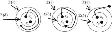
Figure 5.7 Illustration of L-stability (A), L-asymptotic stability (B), and instability (C). ![]() and
and ![]() symbolize n-dimensional balls (spheres) with radii
symbolize n-dimensional balls (spheres) with radii ![]() and
and ![]() , respectively.
, respectively.
Direct Lyapunov method: Let ![]() be the distance of the state
be the distance of the state ![]() from the origin
from the origin ![]() (defined using any valid norm). If we find some distance
(defined using any valid norm). If we find some distance ![]() which tends to zero for
which tends to zero for ![]() , then we conclude that the system is asymptotically stable. To show that a system is asymptotically stable using Lyapunov’s direct method, we do not need to find such a distance (norm), but a Lyapunov function which is actually a generalized energy function.
, then we conclude that the system is asymptotically stable. To show that a system is asymptotically stable using Lyapunov’s direct method, we do not need to find such a distance (norm), but a Lyapunov function which is actually a generalized energy function.
Definition 5.6
Time-invariant Lyapunov function is called any scalar function ![]() of
of ![]() which for all
which for all ![]() and
and ![]() in the vicinity of the origin satisfies the following four conditions:1
in the vicinity of the origin satisfies the following four conditions:1
Theorem 5.3
If a Lyapunov function ![]() can be found for the state of a nonlinear or linear system
can be found for the state of a nonlinear or linear system ![]() , where
, where ![]() (
(![]() is a general function), then the state
is a general function), then the state ![]() is asymptotically stable.■
is asymptotically stable.■
Remarks
(i) If Definition 5.6 holds for all ![]() , then we have “uniformly asymptotic stability.”
, then we have “uniformly asymptotic stability.”
(ii) If the system is linear, or we replace in Definition 5.6 the condition “![]() in the vicinity of the origin,” by the condition “
in the vicinity of the origin,” by the condition “![]() everywhere,” then we have “total asymptotic stability.”
everywhere,” then we have “total asymptotic stability.”
(iii) If the condition (iv) of Definition 5.6 becomes ![]() , then we have (simple) L-stability.
, then we have (simple) L-stability.
Clearly, to establish L-stability of a system, we must find a Lyapunov function. Unfortunately, there does not exist a general methodology for this.
Analogous results hold for the case of time-varying Lyapunov functions ![]() , namely:
, namely:
Definition 5.7
Time-varying Lyapunov function ![]() for the system’s state is any scalar function of
for the system’s state is any scalar function of ![]() and
and ![]() , which, for all
, which, for all ![]() and
and ![]() near the origin
near the origin ![]() , has the following properties:
, has the following properties:
Remark
For all ![]() , the function
, the function ![]() should have values greater than or equal to the values of some continuous nonreducing time-invariant function.
should have values greater than or equal to the values of some continuous nonreducing time-invariant function.
Theorem 5.4
If a time-varying Lyapunov function ![]() can be found for the state
can be found for the state ![]() of the system
of the system ![]() , then the state
, then the state ![]() is asymptotically stable.■
is asymptotically stable.■
Definition 5.8
(i) If the conditions of Definition 5.7 hold for all ![]() and
and ![]() , where
, where ![]() is a continuous nondecreasing scalar function of
is a continuous nondecreasing scalar function of ![]() with
with ![]() , then we have uniformly asymptotic stability.
, then we have uniformly asymptotic stability.
(ii) If the system is linear or the conditions of Definition 5.7 hold everywhere (not only in a region of the origin ![]() ), and if we have
), and if we have ![]() , when
, when ![]() , then we say that the system is uniformly totally asymptotically stable.■
, then we say that the system is uniformly totally asymptotically stable.■
In the case of a linear time-varying system ![]() the Lyapunov (time varying) function
the Lyapunov (time varying) function ![]() is given by the quadratic (energy) function:
is given by the quadratic (energy) function:
![]() (5.14a)
(5.14a)
where ![]() satisfies the following matrix differential equation:
satisfies the following matrix differential equation:
![]() (5.14b)
(5.14b)
If the system is time-invariant ![]() , then
, then ![]() and the above differential equation for
and the above differential equation for ![]() reduces to the following algebraic equation for
reduces to the following algebraic equation for ![]() :
:
![]() (5.15)
(5.15)
In this case, we can select a positive definite matrix ![]() and solve the
and solve the ![]() equations (
equations (![]() is symmetric) for the elements of
is symmetric) for the elements of ![]() . Then, if
. Then, if ![]() (i.e., if
(i.e., if ![]() is positive definite) the system is asymptotically stable.
is positive definite) the system is asymptotically stable.
5.2.3 State Feedback Control
State feedback control is more powerful than classical control because the design of a total controller for a multiple-input multiple-output (MIMO) system is performed in a unified way for all control loops simultaneously, and not serially one loop after the other which does not guarantee the overall system stability and robustness. In this section we will briefly review the eigenvalue placement controller for SISO systems.
Let a SISO system:
![]()
where ![]() is a
is a ![]() constant matrix,
constant matrix, ![]() is an
is an ![]() constant matrix (column vector),
constant matrix (column vector), ![]() is an
is an ![]() matrix (row vector),
matrix (row vector), ![]() is a scalar input, and
is a scalar input, and ![]() is a scalar constant. In this case, a state feedback controller has the form:
is a scalar constant. In this case, a state feedback controller has the form:
![]() (5.16)
(5.16)
where ![]() is a new control input and
is a new control input and ![]() is an n-dimensional constant row vector:
is an n-dimensional constant row vector: ![]() . Introducing this control law into the system, we get the state equations of the closed-loop (feedback) system:
. Introducing this control law into the system, we get the state equations of the closed-loop (feedback) system:
![]() (5.17)
(5.17)
The eigenvalue placement design problem is to select the controller gain matrix ![]() such that the eigenvalues of the closed-loop matrix
such that the eigenvalues of the closed-loop matrix ![]() are placed at desired positions
are placed at desired positions ![]() . It can be shown that this can be done (i.e., the system eigenvalues are controllable by state feedback) if and only if the system
. It can be shown that this can be done (i.e., the system eigenvalues are controllable by state feedback) if and only if the system ![]() is totally controllable. The concept of controllability has been developed to study the ability of a controller to alter the performance of the system in an arbitrary desired way. As it is known, the positions of the eigenvalues specify the performance characteristics of a system.
is totally controllable. The concept of controllability has been developed to study the ability of a controller to alter the performance of the system in an arbitrary desired way. As it is known, the positions of the eigenvalues specify the performance characteristics of a system.
Definition 5.9
A state ![]() of a system is called totally controllable if it can be driven to a final state
of a system is called totally controllable if it can be driven to a final state ![]() as quickly as desired independently of the initial time
as quickly as desired independently of the initial time ![]() . A system is said to be totally controllable if all of its states are totally controllable.■
. A system is said to be totally controllable if all of its states are totally controllable.■
Intuitively, we can see that if some state variables do not depend on the control input ![]() , no way exists that can drive it to some other desired state. Thus, this state is called a noncontrollable state. If a system has at least one noncontrollable state, it is said to be nontotally controllable or, simply, noncontrollable. The above controllability concept refers to the states of a system and so it is characterized as state controllability. If the controllability is referred to the outputs of a system then we have the so-called output controllability. In general, state controllability and output controllability are not the same.
, no way exists that can drive it to some other desired state. Thus, this state is called a noncontrollable state. If a system has at least one noncontrollable state, it is said to be nontotally controllable or, simply, noncontrollable. The above controllability concept refers to the states of a system and so it is characterized as state controllability. If the controllability is referred to the outputs of a system then we have the so-called output controllability. In general, state controllability and output controllability are not the same.
Theorem 5.5
The necessary and sufficient condition for a linear system ![]() to be totally state controllable is that the controllability matrix:
to be totally state controllable is that the controllability matrix:
![]() (5.18a)
(5.18a)
has
![]() (5.18b)
(5.18b)
where ![]() is the dimensionality of the state vector
is the dimensionality of the state vector ![]() .■
.■
The most straightforward technique for selecting the feedback matrix ![]() is through the use of the controllable canonical form. This technique involves the following steps:
is through the use of the controllable canonical form. This technique involves the following steps:
Step 1: We write down the characteristic polynomial ![]() of the matrix
of the matrix ![]() :
:
![]()
Step 2: Then, we find a similarity transformation ![]() that converts the given system to its controllable canonical form
that converts the given system to its controllable canonical form ![]() .
.
Step 3: From the desired eigenvalues of the closed-loop system, we determine the desired characteristic polynomial:
![]()
The feedback gain matrix ![]() of the controllable canonical model is given by:
of the controllable canonical model is given by:
![]()
Step 4: Equating the last rows of ![]() and
and ![]() we find:
we find:
![]()
![]() (5.19)
(5.19)
5.2.4 Second-Order Systems
The state vector ![]() of a second-order system contains the position and velocity of the variable (physical quantity) of interest, namely:
of a second-order system contains the position and velocity of the variable (physical quantity) of interest, namely:
![]()
Suppose that it is desired to design the state feedback controller such that the system’s state follows a desired trajectory ![]() . In this case, the feedback must use the measured error:2
. In this case, the feedback must use the measured error:2
![]() (5.20)
(5.20)
and the controller should reduce the sensitivity of the system to the inaccuracy and the uncertainty in the parameter values used in the dynamic model.
A fundamental characteristic of control systems is the bandwidth ![]() which determines the operation speed of a system and capability of fast trajectory tracking. The greater the bandwidth is the better, but
which determines the operation speed of a system and capability of fast trajectory tracking. The greater the bandwidth is the better, but ![]() should not be very high because it may excite possible high-frequency components that have not been included in the system model.
should not be very high because it may excite possible high-frequency components that have not been included in the system model.
As an example, consider the following simple second-order system:
![]() (5.21)
(5.21)
which by Eq. (5.20) gives the error equation:
![]() (5.22)
(5.22)
Defining the state vector:
![]()
we get the following controllable canonical form:
![]() (5.23a)
(5.23a)
where:
![]() (5.23b)
(5.23b)
To get a desired bandwidth ![]() , we select the desired closed-loop characteristic polynomial as:
, we select the desired closed-loop characteristic polynomial as:
![]() (5.24)
(5.24)
where ![]() is the undamped natural frequency (taken equal to the desired bandwidth
is the undamped natural frequency (taken equal to the desired bandwidth ![]() ) and
) and ![]() is the damping coefficient (usually selected
is the damping coefficient (usually selected ![]() ).
).
Then, the feedback controller is selected as in Eqs. (5.16) and (5.19) with ![]() (unit matrix), namely:
(unit matrix), namely:
![]()
or
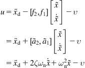 (5.25)
The closed loop error system is obtained using Eqs. (5.22) and (5.25), that is:
![]() (5.26)
(5.26)
which has the desired damping and bandwidth specifications.
The control law (5.25) contains the proportional term ![]() and the derivative term
and the derivative term ![]() , that is, it is a PD (proportional plus derivative controller) which is one of the most popular and efficient controllers. For second-order systems, the PD controller gives exact results.
, that is, it is a PD (proportional plus derivative controller) which is one of the most popular and efficient controllers. For second-order systems, the PD controller gives exact results.
Example 5.2
Consider the case where the system (5.21) is corrupted by a disturbance ![]() as:
as:
![]()
(a) It is desired to determine the steady-state position error ![]() of the closed-loop PD controlled system when
of the closed-loop PD controlled system when ![]() is a step disturbance of amplitude
is a step disturbance of amplitude ![]() :
:
![]()
(b) Show that this steady-state error vanishes if, instead of the PD controller, a PID (proportional plus integral plus derivative) controller is used.
Solution
(a) With the PD controller, the closed-loop disturbed system (5.26) becomes:
![]()
With ![]() and
and ![]() , the above step disturbance, the steady-state position error, obtained by setting
, the above step disturbance, the steady-state position error, obtained by setting ![]() and
and ![]() , satisfies the relation:
, satisfies the relation:
![]()
Thus:
![]()
We see that ![]() has a nonzero finite value which is proportional to
has a nonzero finite value which is proportional to ![]() and inversely proportional to the square of the bandwidth
and inversely proportional to the square of the bandwidth ![]() .
.
(b) If we use a PID controller:
![]()
the closed-loop error system becomes:
![]()
Then, in the limit as ![]() , for
, for ![]() ,
, ![]() and
and ![]() ,
, ![]() we get:
we get:
![]()
which implies ![]() . Otherwise,
. Otherwise, ![]() cannot have a finite value.
cannot have a finite value.
Remark
The above results can also be obtained using the well-known Laplace transform final-value property ![]() and computing
and computing ![]() via the error system’s transfer function.
via the error system’s transfer function.
Example 5.3
It is desired to check the stability of the following systems using the Lyapunov method:
Solution
System (a): This system has the equilibrium state ![]() . We examine if the function
. We examine if the function ![]() is a Lyapunov function. This is done by checking if all conditions for
is a Lyapunov function. This is done by checking if all conditions for ![]() to be a Lyapunov function are satisfied. We have:
to be a Lyapunov function are satisfied. We have:
We see that all properties of the candidate function required to be a Lyapunov function hold, and so the system ![]() is uniformly asymptotically stable.
is uniformly asymptotically stable.
System (b): We try the following candidate Lyapunov function:
![]()
This function has the following properties:
that is, it possesses all properties of a Lyapunov function. Therefore, the only equilibrium state ![]() (i.e., the origin) is totally asymptotically stable.
(i.e., the origin) is totally asymptotically stable.
5.3 General Robot Controllers
The following general controllers, which are standard in robotics [2–4], will be examined:
• Proportional plus derivative control
• Lyapunov function based control
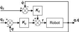
5.3.1 Proportional Plus Derivative Position Control
Here, it will be shown that PD control leads to satisfactory results in the control of the position of a general robot described in Eqs. (3.11a) and (3.11b):
![]()
![]()
where for any ![]() ,
, ![]() is a known positive definite matrix. Assuming that the friction is negligible and omitting the gravity term
is a known positive definite matrix. Assuming that the friction is negligible and omitting the gravity term ![]() , which anyway is zero in mobile robots moving on an horizontal terrain, we get:
, which anyway is zero in mobile robots moving on an horizontal terrain, we get:
![]() (5.27)
(5.27)
where ![]() is defined as in Eq. (3.13), and the matrix
is defined as in Eq. (3.13), and the matrix ![]() is antisymmetric.
is antisymmetric.
Let ![]() be the error between
be the error between ![]() and
and ![]() . Then, the PD controller has the form
. Then, the PD controller has the form
![]() (5.28)
(5.28)
where ![]() and
and ![]() are positive definite symmetric matrices. The resulting feedback control scheme has the form of Figure 5.8.
are positive definite symmetric matrices. The resulting feedback control scheme has the form of Figure 5.8.
Let us try the following candidate Lyapunov function:
![]() (5.29)
(5.29)
where the term ![]() is the robot’s kinetic energy, and the term
is the robot’s kinetic energy, and the term ![]() represents the proportional control term. Thus, the function
represents the proportional control term. Thus, the function ![]() can be considered as representing the total energy of the closed-loop system. Since
can be considered as representing the total energy of the closed-loop system. Since ![]() and
and ![]() are symmetric positive definite matrices, we have
are symmetric positive definite matrices, we have ![]() and
and ![]() for
for ![]() . Therefore, we have to check the validity of property (iv) of Definition 5.6.
. Therefore, we have to check the validity of property (iv) of Definition 5.6.
Here, Eq. (5.29) gives:
 (5.30)
Now, introducing the control law (5.28) into Eq. (5.30) we get:
 (5.31)
Therefore, since the matrix ![]() is antisymmetric, Eq. (5.31) finally gives:
is antisymmetric, Eq. (5.31) finally gives:
![]() (5.32)
(5.32)
We observe that while the Lyapunov function ![]() in Eq. (5.29) depends on
in Eq. (5.29) depends on ![]() , its derivative
, its derivative ![]() depends on
depends on ![]() , which is analogous of the known property of classical SISO PD control. The condition (5.32) ensures that the feedback error control system (Figure 5.8) is L-stable. It is also useful to remark that the PD control (5.28) is particularly robust with respect to mass variations because it does not require knowledge of the parameters that depend on mass.
, which is analogous of the known property of classical SISO PD control. The condition (5.32) ensures that the feedback error control system (Figure 5.8) is L-stable. It is also useful to remark that the PD control (5.28) is particularly robust with respect to mass variations because it does not require knowledge of the parameters that depend on mass.
A special case of the controller (5.28) is:
![]()
which is applied to each joint separately. If the motion is subject to friction (assumed linear) the robot model (5.27) must simply be replaced by:
![]()
where ![]() is the diagonal matrix of friction coefficients. The present PD controller can be enhanced with an integral term as given in Example 5.2.
is the diagonal matrix of friction coefficients. The present PD controller can be enhanced with an integral term as given in Example 5.2.
5.3.2 Lyapunov Stability-Based Control Design
The control design method applied to the above problem is known as Lyapunov-based controller design and constitutes a widely used method for both linear and nonlinear systems. The steps of this method are the following:
Step 1: Select a trial (candidate) Lyapunov function, which is typically some kind of energy-like function for the system, and possesses the first three properties of Lyapunov functions (Definition 5.6, Section 5.2.2).
Step 2: Derive the equation for the derivative ![]() along the system trajectory:
along the system trajectory:
![]()
and select a feedback control law:
![]()
![]()
Typically, ![]() is a nonlinear function of
is a nonlinear function of ![]() that contains some parameters and gains which can be selected to make
that contains some parameters and gains which can be selected to make ![]() , and thus ensures that the closed-loop system is asymptotically stable.
, and thus ensures that the closed-loop system is asymptotically stable.
Remark
For a given system, one may find several Lyapunov functions and corresponding stabilization controllers. If the system is linear time-invariant ![]() , then it is not necessary to work using the Lyapunov method. In this case, the controller is a static linear state feedback controller
, then it is not necessary to work using the Lyapunov method. In this case, the controller is a static linear state feedback controller ![]() (Eq. (5.16)), which can be selected to make the closed-loop matrix a Hurwitz matrix (with all its eigenvalues on the strict left-hand s-plane). This assures that the closed-loop system is asymptotically and exponentially stable. The Lyapunov-based controller design method will be applied as a rule in most cases of the discussions that follow.
(Eq. (5.16)), which can be selected to make the closed-loop matrix a Hurwitz matrix (with all its eigenvalues on the strict left-hand s-plane). This assures that the closed-loop system is asymptotically and exponentially stable. The Lyapunov-based controller design method will be applied as a rule in most cases of the discussions that follow.
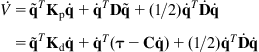
5.3.3 Computed Torque Control
The computed torque control technique reduces the effects of the uncertainty in all the terms of the Lagrange model. The controller ![]() is selected to have the same form as the dynamic model (Eq. (3.11a)), that is:
is selected to have the same form as the dynamic model (Eq. (3.11a)), that is:
![]() (5.33)
(5.33)
Thus, since the inertia matrix is positive definite (and so invertible), introducing the control law (5.33) in the system (3.11a), we get:
![]() (5.34)
(5.34)
This implies that ![]() can be a decoupled controller (PD, PID) that can control each joint (motor axis) independently. The basic problem of the computed torque method is that we do not have available the exact values of
can be a decoupled controller (PD, PID) that can control each joint (motor axis) independently. The basic problem of the computed torque method is that we do not have available the exact values of ![]() ,
, ![]() , and
, and ![]() , but only approximate values
, but only approximate values ![]() ,
, ![]() , and
, and ![]() . Then, instead of Eq. (5.33) we get:
. Then, instead of Eq. (5.33) we get:
![]() (5.35)
(5.35)
and so Eq. (5.34) is replaced by:
![]() (5.36)
(5.36)
A problem with the model in Eq. (5.35) is the investigation of its robustness to modeling uncertainties which include uncertainties in the parameter values and nonmodeled high-frequency components (e.g., structural resonance, sampling rate, or omitted time delays). The computed torque control method belongs to the general class of linearization techniques via nonlinear state feedback (see Section 6.3). Solving the model (Eq. (3.11a)) for ![]() we get:
we get:
![]() (5.37)
(5.37)
Introducing the controller (5.35) into (5.37) we obtain the block diagram of the overall closed-loop system shown in Figure 5.9.
5.3.4 Robot Control in Cartesian Space
The controllers presented thus far work in the joints’ (motors’) space and are based on the error ![]() between the actual and desired generalized joint variables
between the actual and desired generalized joint variables ![]() (called internal variables). The motion of the robot in the Cartesian (or task, or working) space is obtained indirectly from the motion of the joints. However, in many cases, it is required to design the controller so as to work directly with the Cartesian variables, called external variables.
(called internal variables). The motion of the robot in the Cartesian (or task, or working) space is obtained indirectly from the motion of the joints. However, in many cases, it is required to design the controller so as to work directly with the Cartesian variables, called external variables.
In Cartesian space, we have three types of controllers which are known as resolved motion controllers:
Here, we will study the resolved motion rate control which is mostly used in mobile robots. The resolved acceleration controller is actually an extension of the resolved motion rate control that includes the acceleration, a fact that will also be briefly considered.
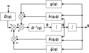
5.3.4.1 Resolved Motion Rate Control
The resolved motion rate control is the control where the joints are moved simultaneously in different velocities, such that a desired motion in Cartesian (or task) space is obtained.
In general, the relation of the linear and angular velocity (motion rate) vector:
![]()
in Cartesian space and the velocities ![]() of the robotic joints is given by the Jacobian relation (Eq. (2.6)):
of the robotic joints is given by the Jacobian relation (Eq. (2.6)):
![]() (5.38)
(5.38)
where the Jacobian matrix ![]() is given by Eq. (2.5), which has the inverse (see Eqs. (2.7b) and (2.8)):
is given by Eq. (2.5), which has the inverse (see Eqs. (2.7b) and (2.8)):
![]() (5.39a)
(5.39a)
or the generalized inverse:
![]() (5.39b)
(5.39b)
Differentiating Eq. (5.38) we get:
![]() (5.40)
(5.40)
Thus, introducing into Eq. (5.40) the expression of ![]() given by Eq. (5.39a) yields:
given by Eq. (5.39a) yields:
![]() (5.41)
(5.41)
This relation gives the accelerations of the joints for given linear/angular velocity and acceleration of the robot end-effector in Cartesian space. If ![]() is not square, we use the generalized inverse
is not square, we use the generalized inverse ![]() in place of
in place of ![]() .
.
The block diagram of the resolved velocity control is shown in Figure 5.10.
Figure 5.10 Block diagram of the robot resolved rate control based on Eq. (5.39a).
In the simplest case, the joints control can be a proportional control law with gain ![]() . In many cases, the task space control is required to be in a coordinate frame attached to the robot (and not in the world coordinate frame). The velocity
. In many cases, the task space control is required to be in a coordinate frame attached to the robot (and not in the world coordinate frame). The velocity ![]() is then given by:
is then given by:
![]() (5.42)
(5.42)
where ![]() is the desired velocity of the robot and
is the desired velocity of the robot and ![]() is a matrix that relates
is a matrix that relates ![]() to
to ![]() . Then, from Eqs. (5.39a) and (5.39b) we get:
. Then, from Eqs. (5.39a) and (5.39b) we get:
![]() (5.43)
(5.43)
The relation (5.43) is typically used in vision-based robot control (visual servoing).
5.3.4.2 Resolved Motion Acceleration Control
The resolved motion acceleration control method is based on the equation:
![]() (5.44)
(5.44)
which is found by differentiating Eq. (5.38). The desired position, velocity, and acceleration of the robot in Cartesian space are assumed to be known from the trajectory planner. Thus, to reduce the position error, we must apply appropriate forces/torques at the robot joints, such that the acceleration in Cartesian space satisfies the relation:
![]() (5.45)
(5.45)
where ![]() , and
, and ![]() are the desired translation position, velocity, and acceleration, respectively.
are the desired translation position, velocity, and acceleration, respectively.
Here, the position error is:
![]()
Therefore, in terms of ![]() , Eq. (5.45) is written as:
, Eq. (5.45) is written as:
![]() (5.46)
(5.46)
and the gains ![]() should be selected such that
should be selected such that ![]() tends asymptotically to zero. A similar error equation can be derived for the angular acceleration
tends asymptotically to zero. A similar error equation can be derived for the angular acceleration ![]() , using the control law:
, using the control law:
![]() (5.47)
(5.47)
where ![]() is the orientation angle in the Cartesian space. Combining Eqs. (5.45) and (5.47), and inserting into Eq. (5.44), we get:
is the orientation angle in the Cartesian space. Combining Eqs. (5.45) and (5.47), and inserting into Eq. (5.44), we get:
![]() (5.48)
(5.48)
where:
![]()
Equation (5.48) constitutes the basis for the resolved motion acceleration control of robots. The position ![]() and velocity
and velocity ![]() are measured by potentiometers or optical encoders.
are measured by potentiometers or optical encoders.
5.4 Control of Differential Drive Mobile Robot
The control procedure will involve two stages:
The resulting linear and angular velocities in the kinematic stage will be used as reference inputs for the dynamic stage. Thus, this procedure belongs to the general class of backstepping control [5–13].
5.4.1 Nonlinear Kinematic Tracking Control
The robot motion is governed by the dynamic model (Eqs. (3.23a) and (3.23b), the kinematic model (Eq. (2.26)), and the nonholonomic constraint (Eq. (2.27)), namely:
![]() (5.49a)
(5.49a)
![]() (5.49b)
(5.49b)
![]() (5.49c)
(5.49c)
where, for notational simplicity, the index ![]() was dropped from
was dropped from ![]() ,
, ![]() and
and ![]() ,
, ![]() ,
, ![]() are the control inputs, with:
are the control inputs, with:
![]() (5.49d)
(5.49d)
being the state vector.
The problem is to track a desired state trajectory:
![]() (5.50)
(5.50)
with error that goes asymptotically to zero.
To this end, the Lyapunov stabilizing method will be used. For realizability, the desired trajectory must satisfy both the kinematic equations and the nonholonomic constraint, that is:3
 (5.51)
The errors ![]() ,
, ![]() , and
, and ![]() , expressed in the wheeled mobile robots’ (WMR’s) local (moving) coordinate frame
, expressed in the wheeled mobile robots’ (WMR’s) local (moving) coordinate frame ![]() , are given by (see Eq. (2.17)):
, are given by (see Eq. (2.17)):
![]() (5.52a)
(5.52a)
and
![]() (5.52b)
(5.52b)
Differentiating Eqs. (5.52a) and (5.52b) and taking into account Eqs. (5.49c) and (5.51), we get the following kinematic model for the error ![]() :
:
 (5.53)
where the linear and angular velocities ![]() and
and ![]() are the kinematic control variables. Clearly, Eq. (5.53) satisfies the kinematic and nonholonomic equations of the WMR.
are the kinematic control variables. Clearly, Eq. (5.53) satisfies the kinematic and nonholonomic equations of the WMR.
Therefore, the kinematic feedback controller will be based on Eq. (5.53). The Lyapunov stabilizing method of Section 5.3.2 will be applied. Since here the controller should be nonlinear, we cannot select its structure beforehand. Its structure will be determined by the choice of the candidate Lyapunov function. Here, the following candidate function is selected [14]:
![]() (5.54)
(5.54)
This function satisfies the first three properties of Lyapunov functions, namely:
We therefore have to check under what conditions the fourth property can be satisfied.
Differentiating Eq. (5.54) with respect to time we get:
![]() (5.55)
(5.55)
To make ![]() , the control inputs
, the control inputs ![]() and
and ![]() are selected such that:
are selected such that:
![]() (5.56)
(5.56)
which leads to:
![]() (5.57a)
(5.57a)
![]() (5.57b)
(5.57b)
Clearly, for ![]() and
and ![]() , we have
, we have ![]() with the equality obtained only when
with the equality obtained only when ![]() and
and ![]() . Thus, the controller (5.57a) and ((5.57b) guarantees total asymptotic tracking to the desired trajectory.
. Thus, the controller (5.57a) and ((5.57b) guarantees total asymptotic tracking to the desired trajectory.
Remark 1
We can also add a gain ![]() in the second term of Eq. (5.56b), that is, choose
in the second term of Eq. (5.56b), that is, choose ![]() as
as
![]() (5.58a)
(5.58a)
In this case, total asymptotic tracking to the desired trajectory ![]() can be proved using the following Lyapunov function:
can be proved using the following Lyapunov function:
![]() (5.58b)
(5.58b)
Remark 2
A more general kinematic controller can be obtained by using the Lyapunov function:
![]() (5.58c)
(5.58c)
with ![]() ,
, ![]() , and
, and ![]() . In the following, we will derive this controller. To this end, we define new control variables
. In the following, we will derive this controller. To this end, we define new control variables ![]() ,
, ![]() and write the model (5.53) as:
and write the model (5.53) as:
![]() (5.58d)
(5.58d)
Differentiating Eq. (5.58c) and using the model (5.58d) we get:

To assure that ![]() , we use two functions
, we use two functions ![]() and
and ![]() for all
for all ![]() , and select
, and select ![]() and
and ![]() such that:
such that:
![]() (5.58e)
(5.58e)
Then, it follows that:
![]()
The above controller assures that ![]() and
and ![]()
![]() . Since
. Since ![]() is uniformly continuous, Barbalat’s Lemma (Sec. 6.2.3) implies that
is uniformly continuous, Barbalat’s Lemma (Sec. 6.2.3) implies that ![]() . This by Eq. (5.58e) implies that
. This by Eq. (5.58e) implies that ![]() and
and ![]()
![]() . Now, obviously,
. Now, obviously, ![]() (i.e.,
(i.e., ![]() ). One way to overcome the fact that
). One way to overcome the fact that ![]() does not converge only to 0 but also to
does not converge only to 0 but also to ![]() is to take care that the WMR, before trying to track immediately the desired trajectory (i.e., the virtual WMR), is rotating about its own axis with an increasing angular velocity
is to take care that the WMR, before trying to track immediately the desired trajectory (i.e., the virtual WMR), is rotating about its own axis with an increasing angular velocity ![]() until it sees the virtual robot. The reader can verify that this can be done by the controller [11]:
until it sees the virtual robot. The reader can verify that this can be done by the controller [11]:
![]()
where ![]() is given by the dynamic model:
is given by the dynamic model:
![]()
with ![]() being a step input function defined by:
being a step input function defined by:
![]()
5.4.2 Dynamic Tracking Control
Having selected ![]() and
and ![]() as in Eqs. (5.57a) and (5.57b) (or Eq. (5.58a)), we select the control inputs (torques)
as in Eqs. (5.57a) and (5.57b) (or Eq. (5.58a)), we select the control inputs (torques) ![]() and
and ![]() in Eq. (5.49a) as:
in Eq. (5.49a) as:
![]() (5.59a)
(5.59a)
![]() (5.59b)
(5.59b)
where:
![]() (5.59c)
(5.59c)
Introducing Eqs. (5.59a)–(5.59c) into Eqs. (5.49a) and (5.49b) we get the velocities’ error equations:
![]()
which for ![]() and
and ![]() are stable and
are stable and ![]() ,
, ![]() converge to zero asymptotically. Therefore, in selecting the feedback control inputs (torques) as in Eqs. (5.59a) and (5.59b) with
converge to zero asymptotically. Therefore, in selecting the feedback control inputs (torques) as in Eqs. (5.59a) and (5.59b) with ![]() and
and ![]() given by Eqs. (5.57a) and (5.57b), the tracking of the desired trajectory
given by Eqs. (5.57a) and (5.57b), the tracking of the desired trajectory ![]() is achieved asymptotically, as required. The block diagram of the feedback tracking controller is depicted in Figure 5.11.
is achieved asymptotically, as required. The block diagram of the feedback tracking controller is depicted in Figure 5.11.

5.5 Computed Torque Control of Differential Drive Mobile Robot
The control design procedure involves again two stages: kinematic control followed by dynamic control. We will work on the WMR shown in Figure 5.12, where the motor dynamics includes a gear box (of ratio N) [13].
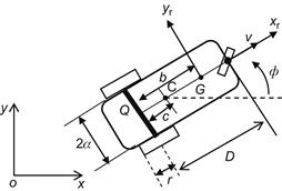
Here, Q is the midpoint of wheel baseline, G the center of gravity, and C the point traced by the controller (different than the point Q).
The meaning of the remaining symbols are self-evident (the same as in Figure 2.7).
5.5.1 Kinematic Tracking Control
The kinematic equations of the robot are:
![]() (5.60a)
(5.60a)
![]() (5.60b)
(5.60b)
![]() (5.60c)
(5.60c)
where ![]() is the lateral velocity in the local coordinate frame
is the lateral velocity in the local coordinate frame ![]() .
.
Equations (5.60a) and (5.60b) are written in the matrix form:
![]()
Now, using new control variables ![]() and
and ![]() defined by:
defined by:
![]() (5.61)
(5.61)
![]() (5.62)
(5.62)
The dynamic system (5.62) is linear and decoupled, and so the state-feedback law:
![]() (5.63)
(5.63)
yields the error dynamics:
![]() (5.64)
(5.64)
with ![]() and
and ![]() .
.
Therefore, from Eq. (5.64), it follows that for any positive gains:
![]()
the tracking error tends exponentially to zero.
Combining Eqs. (5.61) and (5.63) we get the overall nonlinear kinematic control law:
![]() (5.65)
(5.65)
5.5.2 Dynamic Tracking Control
The feedback kinematic controller (5.65) incorporates the WMR kinematic equations and so one can now use the reduced (unconstrained) dynamic model ((3.19a) and (3.19b)) of the robot for the selection of the control inputs (motor torques or motor voltages), as described in Section 5.4.2, where actually the computed torque method was applied.
For the robot of Figure 5.12, with the motor dynamics included, the reduced model has the following form:
![]() (5.66)
(5.66)
where:
![]() (5.67)
(5.67)
 (5.68)
![]() =combined wheel, motor rotor, and gearbox inertia
=combined wheel, motor rotor, and gearbox inertia
![]() =combined wheel, motor, and gearbox friction coefficient
=combined wheel, motor, and gearbox friction coefficient
Now, applying the computed torque (linearization) technique to Eq. (5.66), we choose the voltage control vector ![]() as:
as:
![]() (5.69)
(5.69)
where ![]() is the new control vector. Introducing Eq. (5.69) into Eq. (5.66) we get:
is the new control vector. Introducing Eq. (5.69) into Eq. (5.66) we get:
![]()
with:
![]()
Therefore, selecting the linear state feedback control law:
![]() (5.70)
(5.70)
![]()
which for ![]() is asymptotically stable with equilibrium state
is asymptotically stable with equilibrium state ![]() .
.
Combining Eq. (5.69) with Eq. (5.70), we get the full dynamic controller:
![]() (5.71)
(5.71)
The overall tracking controller of the robot is given by Eqs. (5.65) and (5.71).
Example 5.4
It is desired to formulate and solve the kinematic problem of a unicycle-like WMR to go asymptotically from an initial state (position and orientation) to a goal state (position and orientation) using polar coordinates.
Solution
The unicycle-like robots are described by the kinematic Eq. (2.26):
![]() (5.72)
(5.72)
where ![]() is the velocity and
is the velocity and ![]() is the angle of the WMR
is the angle of the WMR ![]() axis with the goal (world) coordinate frame x-axis. All WMRs with the above kinematic equations, for example, the differential drive WMR, are said to belong to the unicycle-like class of mobile robots. The geometry of the WMR that will be used for formulating the polar coordinates is shown in Figure 5.13 [15].
axis with the goal (world) coordinate frame x-axis. All WMRs with the above kinematic equations, for example, the differential drive WMR, are said to belong to the unicycle-like class of mobile robots. The geometry of the WMR that will be used for formulating the polar coordinates is shown in Figure 5.13 [15].

Figure 5.13 Polar coordinates of the unicycle. Here, the goal coordinate frame Gxy is considered to be the world coordinate frame.
The kinematic control variables of the robot are ![]() and
and ![]() . The polar coordinates (position and orientation) of the WMR are its distance
. The polar coordinates (position and orientation) of the WMR are its distance ![]() from the goal, and its orientation
from the goal, and its orientation ![]() with respect to the goal’s coordinate frame Gxy. The steering angle is
with respect to the goal’s coordinate frame Gxy. The steering angle is ![]() . Then, in polar coordinates, the kinematic model in Eq. (5.72) is replaced by:
. Then, in polar coordinates, the kinematic model in Eq. (5.72) is replaced by:
![]() (5.73a)
(5.73a)
![]() (5.73b)
(5.73b)
![]() (5.73c)
(5.73c)
These relations hold for ![]() , a condition which will be always satisfied by an asymptotic reduction of
, a condition which will be always satisfied by an asymptotic reduction of ![]() to zero (since for any finite time there always be
to zero (since for any finite time there always be ![]() ).
).
Our goal tracking control problem is to find a state-feedback law:
![]() (5.74)
(5.74)
which guarantees that ![]() ,
, ![]() , and
, and ![]() , asymptotically.
, asymptotically.
To this end, we will apply the Lyapunov-based control method. Let us choose the following candidate Lyapunov function [15]:
![]()
 (5.75)
Clearly, the function ![]() possesses the first three properties of Lyapunov functions. We will determine the controller (5.74) which will assure that the fourth property
possesses the first three properties of Lyapunov functions. We will determine the controller (5.74) which will assure that the fourth property ![]() is also possessed by
is also possessed by ![]() , along the system trajectory.
, along the system trajectory.
The time derivative of ![]() , along the trajectory determined by Eqs. (5.73a)–(5.73c), is found to be:
, along the trajectory determined by Eqs. (5.73a)–(5.73c), is found to be:
![]() (5.76a)
(5.76a)
where:
![]() (5.76b)
(5.76b)
 (5.76c)
Choosing ![]() as:
as:
![]() (5.77)
(5.77)
yields:
![]() (5.78)
(5.78)
Now, introducing Eq. (5.77) into Eq. (5.76c) we get:
![]()
Thus, selecting ![]() as:
as:
![]() (5.79)
(5.79)
yields:
![]() (5.80)
(5.80)
The inequalities (5.78) and (5.80) give:
![]() (5.81)
(5.81)
This implies, by the Lyapunov stability theorem, that ![]() and
and ![]() go asymptotically to zero for any
go asymptotically to zero for any ![]() . Thus, we have to see what happens to
. Thus, we have to see what happens to ![]() . To this end, we get the closed-loop system kinematics by introducing the control laws (5.77) and ((5.79)) into Eqs. (5.73a)–(5.73c), namely:
. To this end, we get the closed-loop system kinematics by introducing the control laws (5.77) and ((5.79)) into Eqs. (5.73a)–(5.73c), namely:
![]() (5.82a)
(5.82a)
![]() (5.82b)
(5.82b)
![]() (5.82c)
(5.82c)
These equations show that the asymptotic convergence of ![]() and
and ![]() to zero implies the asymptotic convergence of
to zero implies the asymptotic convergence of ![]() to its only equilibrium state
to its only equilibrium state ![]() . In fact, from Eq. (5.82c) it follows that
. In fact, from Eq. (5.82c) it follows that ![]() implies
implies ![]() , that is,
, that is, ![]() tends to some finite value
tends to some finite value ![]() . Then, we see from Eq. (5.82b) that the uniformly continuous function
. Then, we see from Eq. (5.82b) that the uniformly continuous function ![]() tends necessarily to
tends necessarily to ![]() .4 On the other hand, by Barbalat’s lemma,
.4 On the other hand, by Barbalat’s lemma, ![]() tends to zero, which in turn implies that
tends to zero, which in turn implies that ![]() (see Section 6.2.3). Therefore, the smooth kinematic control laws (5.77) and ((5.79)) assure the asymptotic tracking of the goal position and orientation by the WMR, as desired. The fact that the control laws (5.77) and ((5.79)) are continuously differentiable does not contradict Brockett’s Theorem 6.6 and its corollary (c) because this theorem is valid for the Cartesian state-space representation (Eq. (5.72)) of the unicycle-like WMR [15].
(see Section 6.2.3). Therefore, the smooth kinematic control laws (5.77) and ((5.79)) assure the asymptotic tracking of the goal position and orientation by the WMR, as desired. The fact that the control laws (5.77) and ((5.79)) are continuously differentiable does not contradict Brockett’s Theorem 6.6 and its corollary (c) because this theorem is valid for the Cartesian state-space representation (Eq. (5.72)) of the unicycle-like WMR [15].
4Recall that ![]() as
as ![]() .
.
5.6 Car-Like Mobile Robot Control
For the car-like WMR, we will study the following two representative problems:
5.6.1 Parking Control
Consider a car-like WMR (Figure 2.9) which controls the steering angle ![]() and the rear-wheels’ velocity
and the rear-wheels’ velocity ![]() . The orientation of the car body (i.e., of
. The orientation of the car body (i.e., of ![]() ) is
) is ![]() . The kinematic equations of the robot are given by Eq. (2.52):
. The kinematic equations of the robot are given by Eq. (2.52):
 (5.83)
The problem is to control the WMR (using ![]() and
and ![]() ) so as to move it to a desired parking position and orientation, which here is assumed to be
) so as to move it to a desired parking position and orientation, which here is assumed to be ![]() ,
, ![]() , and
, and ![]() (as it was actually done in Example 5.4 for the unicycle WMR). Here, this problem will be solved by a two-step maneuver to overcome the turning radius limitation of the car-like mobile robot, namely [16]:
(as it was actually done in Example 5.4 for the unicycle WMR). Here, this problem will be solved by a two-step maneuver to overcome the turning radius limitation of the car-like mobile robot, namely [16]:
Use of the Lyapunov-based control method will again be made as usual.
Step 1:![]() control
control
We select the following candidate Lyapunov function:
![]()
which satisfies the first three conditions of Lyapunov functions. We will check if the third condition can be satisfied, along the trajectory of the system in Eq. (5.83). We have:
 (5.84)
Choosing:
 (5.85)
and introducing into Eq. (5.84) yields:
![]() (5.86)
(5.86)
which, by Lyapunov theorem, implies that ![]() tends asymptotically to zero.
tends asymptotically to zero.
The closed loop kinematics equation is:
![]() (5.87)
(5.87)
Let ![]() . For
. For ![]() to stay zero,
to stay zero, ![]() should be zero. Then, Eq. (5.87) implies that
should be zero. Then, Eq. (5.87) implies that ![]() should also tend to zero, for
should also tend to zero, for ![]() .
.
The change of the sign of ![]() is needed when the WMR cannot move with its current velocity due to the presence of obstacles or when the measured states exceed some predetermined bounds. Of course, the initial selection of
is needed when the WMR cannot move with its current velocity due to the presence of obstacles or when the measured states exceed some predetermined bounds. Of course, the initial selection of ![]() affects the efficiency of the path. Actually, the controller (5.85) is a nonlinear bang-bang controller. Therefore, a switching rule is needed to determine when the change from
affects the efficiency of the path. Actually, the controller (5.85) is a nonlinear bang-bang controller. Therefore, a switching rule is needed to determine when the change from ![]() to
to ![]() must occur.
must occur.
Defining ![]() , the switching rule is:
, the switching rule is:
This rule means that if the front part of the WMR is closer to the origin, then it will go forward or backward.
Step 2:![]() control
control
We use the same form of the candidate Lyapunov function:
![]()
with ![]() and
and ![]() .
.
The time derivative ![]() along the trajectory of Eq. (5.83) is:
along the trajectory of Eq. (5.83) is:
![]()
Choosing:
![]() (5.88)
(5.88)
gives:
 (5.89)
which is negative semidefinite for ![]() .
.
For ![]() , in which case, by Eq. (5.88),
, in which case, by Eq. (5.88), ![]() , we have
, we have
![]()
Therefore, the mobile robot is uniformly L-stable at ![]() . However,
. However, ![]() cannot converge without increasing
cannot converge without increasing ![]() , a fact which is due to the low bound of the WMR turning radius (Figure 5.14A) [16,17]. Actually,
, a fact which is due to the low bound of the WMR turning radius (Figure 5.14A) [16,17]. Actually, ![]() can be made arbitrarily small at the first step. Therefore, when we achieve a very small
can be made arbitrarily small at the first step. Therefore, when we achieve a very small ![]() (i.e.,
(i.e., ![]() ), we use
), we use ![]() , and
, and ![]() .
.
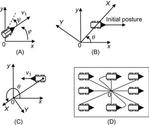
Figure 5.14 (A) For ![]() to converge,
to converge, ![]() must be increased. (B) Case
must be increased. (B) Case ![]() . (C) Case
. (C) Case ![]() . (D) Convergence to the origin
. (D) Convergence to the origin ![]() using Eq. (5.90).
using Eq. (5.90).
This situation is overcome if we use the transformation [16]:
![]() (5.90)
(5.90)
In this way, the distance from the origin to the WMR is equal to the error of ![]() , and the difference angle of the WMR with the x-axis becomes the error of
, and the difference angle of the WMR with the x-axis becomes the error of ![]() . As shown in Figure 5.14D, the controller (5.88) with the above switching type transformation assures that the WMR can go to
. As shown in Figure 5.14D, the controller (5.88) with the above switching type transformation assures that the WMR can go to ![]() starting from any initial posture.
starting from any initial posture.
5.6.2 Leader–Follower Control
Consider two car-like robots that follow a path with the first car acting as the leader and the second being a follower (Figure 5.15). For more WMRs, one following the other in front of it, this problem is known as formation control [7].
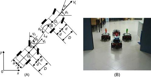
Figure 5.15 (A) Two car-like WMRs (leader–follower structure). (B) Four WMRs in a typical formation (diamond structure). Source: www.robot.uji.es/lab/plone/research/pnebot/index_html2.
The leader–follower control problem under consideration is to find a velocity control input for the follower that assures convergence of the relative distance ![]() and relative bearing angle
and relative bearing angle ![]() of the WMRs to their desired values, under the assumption that the leader motion is known and is the result of an independent control law [7]. To solve the problem, we will apply the Lyapunov-based control design method using the kinematic and dynamic equations of the bicycle equivalent presented in Section 3.4 (see Eqs. (3.56), (3.57), (3.60a)–(3.60d)).
of the WMRs to their desired values, under the assumption that the leader motion is known and is the result of an independent control law [7]. To solve the problem, we will apply the Lyapunov-based control design method using the kinematic and dynamic equations of the bicycle equivalent presented in Section 3.4 (see Eqs. (3.56), (3.57), (3.60a)–(3.60d)).
In Figure 5.15, ![]() ,
, ![]() , and
, and ![]() are the linear velocity, orientation angle, and steering angle of the leader, and
are the linear velocity, orientation angle, and steering angle of the leader, and ![]() ,
, ![]() ,
, ![]() are the respective variables of the follower. The coordinates of points
are the respective variables of the follower. The coordinates of points ![]() and
and ![]() are denoted by
are denoted by ![]() and
and ![]() .
.
We first derive the dynamic equations for the errors:
![]() (5.91)
(5.91)
where ![]() ,
, ![]() , and
, and ![]() represent the desired trajectory of the follower in world coordinates, which are transformed to
represent the desired trajectory of the follower in world coordinates, which are transformed to ![]() ,
, ![]() , and
, and ![]() in the local coordinate frame of the follower. From Figure 5.15 we get:
in the local coordinate frame of the follower. From Figure 5.15 we get:
![]() (5.92a)
(5.92a)
![]() (5.92b)
(5.92b)
![]() (5.92c)
(5.92c)
![]() (5.92d)
(5.92d)
Differentiating Eqs. (5.92b) and (5.92c) gives:
![]() (5.93a)
(5.93a)
![]() (5.93b)
(5.93b)
with (see Eqs. (3.56) and (3.57)):
![]() (5.93c)
(5.93c)
where ![]() .
.
Using Eqs. (3.56) and (5.93c) in Eqs. (5.93a) and (5.93b), we obtain:
![]() (5.94a)
(5.94a)
![]() (5.94b)
(5.94b)
while from Figure 5.13 we have:
![]() (5.95)
(5.95)
Then, differentiating Eqs. (5.92a) and (5.92d), introducing Eqs. (5.94a) and (5.94b), and using the auxiliary variable:
![]()
we get, after some algebraic manipulation:
![]() (5.96a)
(5.96a)
![]() (5.96b)
(5.96b)
Using Figure 5.15, the actual and desired coordinates of the follower’s point A can be expressed in terms of the coordinates of the leader’s point B. Therefore, we use the variables ![]() and
and ![]() and get the error equations (in the world coordinate frame):
and get the error equations (in the world coordinate frame):
![]() (5.97a)
(5.97a)
![]() (5.97b)
(5.97b)
![]() (5.97c)
(5.97c)
Finally, differentiating Eqs. (5.97a)–(5.97c), we obtain the dynamic equations for ![]() ,
, ![]() , and
, and ![]() :
:
![]() (5.98a)
(5.98a)
![]() (5.98b)
(5.98b)
![]() (5.98c)
(5.98c)
We are now ready to apply the usual two-stage (kinematic, dynamic) backstep controller design.
5.6.2.1 Kinematic Controller
We select the candidate Lyapunov function [7]:
![]() (5.99)
(5.99)
which is similar to Eq. (5.54), which possesses the first three properties of Lyapunov functions. The feedback control inputs ![]() and
and ![]() will be selected such that to make
will be selected such that to make ![]() . Differentiating Eq. (5.99) gives:
. Differentiating Eq. (5.99) gives:
![]() (5.100)
(5.100)
Introducing Eqs. (5.98a)–(5.98c) into Eq. (5.100), we find that the selection of ![]() and
and ![]() as:
as:
![]() (5.101a)
(5.101a)
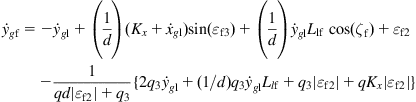 (5.101b)
with ![]() makes
makes ![]() . Indeed, introducing Eqs. (5.98a)–(5.98c), (5.101a), and (5.101b) into Eq. (5.100) yields:
. Indeed, introducing Eqs. (5.98a)–(5.98c), (5.101a), and (5.101b) into Eq. (5.100) yields:
![]()
5.6.2.2 Dynamic Controller
Use will be made of the dynamic model (Eqs. (3.60a)–(3.60d)). The desired velocity and steering angle ![]() ,
, ![]() of the follower are given by the results of the kinematic controller. We define the error:
of the follower are given by the results of the kinematic controller. We define the error:
![]() (5.102)
(5.102)
From Eqs. (3.60a)–(3.60c), applied to the follower WMR, we get:
![]() (5.103)
(5.103)
where ![]() is the driving torque of the steering wheel of radius
is the driving torque of the steering wheel of radius ![]() , and the relation
, and the relation ![]() was used. Combining Eqs. (5.103) and (3.60d) gives:
was used. Combining Eqs. (5.103) and (3.60d) gives:
![]() (5.104)
(5.104)
where:
![]()
![]()
![]()
Subtracting both sides of Eq. (5.104) from ![]() we get:
we get:
![]()
Now, adding and subtracting ![]() to the right-hand side of this equation yields:
to the right-hand side of this equation yields:
![]() (5.105a)
(5.105a)
where:
![]() (5.105b)
(5.105b)
The torque ![]() in Eq. (5.105a) can be found using the computed torque technique as:
in Eq. (5.105a) can be found using the computed torque technique as:
![]() (5.106)
(5.106)
which is introduced into Eq. (5.105a) to give the closed-loop error equation:
![]() (5.107)
(5.107)
It only remains to select ![]() such that
such that ![]() tends to zero asymptotically. We select the candidate Lyapunov function:
tends to zero asymptotically. We select the candidate Lyapunov function:
![]() (5.108)
(5.108)
where ![]() is given by Eq. (5.99).
is given by Eq. (5.99).
Differentiating ![]() and introducing the result into Eq. (5.107) gives:
and introducing the result into Eq. (5.107) gives:
![]()
Since ![]() by the kinematic controller design, we can assure that
by the kinematic controller design, we can assure that ![]() by selecting the gain matrix
by selecting the gain matrix ![]() such that the matrix
such that the matrix ![]() is positive definite, that is:
is positive definite, that is:
![]()
with ![]() and
and ![]() . Then, we find:
. Then, we find:
![]()
This implies that the error ![]() in Eq. (5.105a) tends asymptotically to zero, that is,
in Eq. (5.105a) tends asymptotically to zero, that is, ![]() and
and ![]() , as required. The function
, as required. The function ![]() in the control law Eq. (5.106) can be approximated by a neural network using a weight updating rule as described in Section 8.5 [7].
in the control law Eq. (5.106) can be approximated by a neural network using a weight updating rule as described in Section 8.5 [7].
5.7 Omnidirectional Mobile Robot Control
We will consider the three-wheel omnidirectional dynamic robot model (Eqs. (3.77a) and (3.77b)) derived in Section 3.5:
![]() (5.109)
(5.109)
and will apply the resolved motion acceleration technique, combined with PI or PD control [18]. Solving Eq. (5.109) for ![]() , we get the inverse dynamic resolved acceleration equations:
, we get the inverse dynamic resolved acceleration equations:
![]() (5.110a)
(5.110a)
![]() (5.110b)
(5.110b)
![]() (5.110c)
(5.110c)
where:
![]() (5.111a)
(5.111a)
![]() (5.111b)
(5.111b)
![]() (5.111c)
(5.111c)
with:
![]()
being the errors between the desired and actual trajectories, and ![]() ,
, ![]() ,
, ![]() being proportional gains,
being proportional gains, ![]() ,
, ![]() integral gains, and
integral gains, and ![]() the derivative (velocity) gain of
the derivative (velocity) gain of ![]() . Note that the factors
. Note that the factors ![]() and
and ![]() in Eqs. (5.110a)–(5.110c) are always nonzero (see Eqs. (3.76a)–(3.76c)) and so the above resolved acceleration controllers
in Eqs. (5.110a)–(5.110c) are always nonzero (see Eqs. (3.76a)–(3.76c)) and so the above resolved acceleration controllers ![]() ,
, ![]() , and
, and ![]() exist for all
exist for all ![]() .5
.5
The block diagram of the overall feedback control WMR system is shown in Figure 5.16.
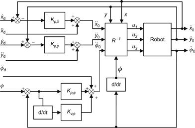
Figure 5.16 Resolved acceleration control system for the three-wheel omnidirectional robot (![]() represents the robot inverse dynamics Eqs. (5.110a)–(5.110c)).
represents the robot inverse dynamics Eqs. (5.110a)–(5.110c)).
The above controller was applied to a real robot with physical parameters:
![]()
The initial state used is:
![]()
A basic experiment was to check the WMRs holonomic property, that is, the ability of the robot to independently achieve translational and rotational motion around the center of gravity in the x-y plane.
To check this property, it was assumed that the robot must travel with a single azimuth ![]() (see Figure 3.6) for 20 s, but with zero rotational angle for 0–10 s, and a uniformly varying rotational angle from
(see Figure 3.6) for 20 s, but with zero rotational angle for 0–10 s, and a uniformly varying rotational angle from ![]() to
to ![]() for 10–20 s. Although the moving velocity was to be
for 10–20 s. Although the moving velocity was to be ![]() in the steady state, a sinusoidal reference velocity was set for each 2 s at the starting and ending period. Using these
in the steady state, a sinusoidal reference velocity was set for each 2 s at the starting and ending period. Using these ![]() and
and ![]() values, the corresponding
values, the corresponding ![]() and
and ![]() were derived from:
were derived from:
![]()
where the positive rotational direction of motion is the counterclockwise direction. The desired accelerations ![]() and
and ![]() were derived by differentiation of
were derived by differentiation of ![]() and
and ![]() . A selection of the gains used is given in Table 5.1.
. A selection of the gains used is given in Table 5.1.

The responses obtained for ![]() ,
, ![]() , and
, and ![]() , and the (x,y) trajectory are shown in Figure 5.17.
, and the (x,y) trajectory are shown in Figure 5.17.
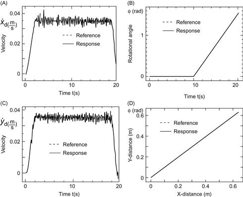
Figure 5.17 (A,C) Actual velocity responses compared to the desired velocity responses ![]() and
and ![]() . (B) Trajectory of
. (B) Trajectory of ![]() , (D) (x,y) trajectory. Source: Reprinted from Ref. [18], with permission from Springer Science+Business Media BV.
, (D) (x,y) trajectory. Source: Reprinted from Ref. [18], with permission from Springer Science+Business Media BV.
We observe that despite the occurrence of some oscillations in the velocities ![]() and
and ![]() , the
, the ![]() trajectory matches perfectly the desired trajectory
trajectory matches perfectly the desired trajectory ![]() . Another experiment was carried out to follow a circular path with a radius less than half the distance between the wheels (say 0.1 m with distance between the wheels 0.356 m). Using the same gains as before, the results were very good, with perfect tracking of the circular path [18].
. Another experiment was carried out to follow a circular path with a radius less than half the distance between the wheels (say 0.1 m with distance between the wheels 0.356 m). Using the same gains as before, the results were very good, with perfect tracking of the circular path [18].
Example 5.5
Apply the computed torque technique to derive a PD path tracking controller for a three-wheel omnidirectional robot.
Solution
We will work with the dynamic model derived for the omnidirectional robot of Figure 3.7 in Example 3.2, namely:
![]() (5.112)
(5.112)
The computed torque control law has the form (Eq. (5.33)):
![]() (5.113)
(5.113)
and the PD control has the form:
![]() (5.114)
(5.114)
where:
![]() (5.115)
(5.115)
is the tracking error of the resulting path from the desired path ![]() . Combining Eqs. (5.113) and (5.114) and introducing into Eq. (5.112), we get the closed-loop system:
. Combining Eqs. (5.113) and (5.114) and introducing into Eq. (5.112), we get the closed-loop system:
![]()
or the tracking error dynamic equation:
![]() (5.116)
(5.116)
since the matrix ![]() is nonsingular. We see that the origin
is nonsingular. We see that the origin ![]() is an equilibrium point of this system. Therefore, selecting proper values of
is an equilibrium point of this system. Therefore, selecting proper values of ![]() and
and ![]() , we can assure that
, we can assure that ![]() tends to zero, that is,
tends to zero, that is, ![]() , asymptotically. To this end, we use the following candidate Lyapunov function:
, asymptotically. To this end, we use the following candidate Lyapunov function:
![]() (5.117)
(5.117)
which, for sufficiently small constant ![]() , satisfies the first two properties of Lyapunov functions.
, satisfies the first two properties of Lyapunov functions.
We will now examine under what conditions ![]() is negative. The time derivative of
is negative. The time derivative of ![]() along the trajectory of
along the trajectory of ![]() is found to be:
is found to be:
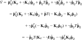
Choosing ![]() and
and ![]() (positive definite), we get
(positive definite), we get ![]() and so
and so ![]() asymptotically.
asymptotically.
The performance of the controller was tested on the WMR of Section 5.7 with the same values of physical parameters and the same desired path using the PD gains given in Table 5.2.
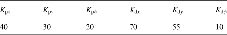
The responses obtained for the ![]() and
and ![]() trajectories are similar to those shown in Figure 5.17. As an exercise, the reader may test the performance of the controller for a circular desired path with a given radius
trajectories are similar to those shown in Figure 5.17. As an exercise, the reader may test the performance of the controller for a circular desired path with a given radius ![]() (e.g.,
(e.g., ![]() ). A parameterized form of the circle equation, namely,
). A parameterized form of the circle equation, namely, ![]() ,
, ![]() can be used where
can be used where ![]() is the angle of the point
is the angle of the point ![]() with reference to the x-axis of the world coordinate frame. In this case, a suitable polynomial or other series representation of the angle
with reference to the x-axis of the world coordinate frame. In this case, a suitable polynomial or other series representation of the angle ![]() can be used. A more complex desired path that might be examined is an 8 shaped path of a given size.
can be used. A more complex desired path that might be examined is an 8 shaped path of a given size.
References
1. Ogata K. State space analysis of control systems Upper Saddle River, NJ: Prentice Hall; 1997.
2. Asada H, Slotine JJ. Robot analysis and control New York, NY: Wiley; 1986.
3. Spong MW, Vidyasagar M. Robot dynamics and control New York, NY: Wiley; 1989.
4. Wolovich W. Robotics: Basic Analysis and Design. Birmingham, UK: Holt Rinehart and Winston, Dreyden Press;1987.
5. Kanayama Y, Kimura Y, Noguchi T. A stable tracking control method for a nonholonomic mobile robot. IEEE Trans Robot Autom. 1991;7:1236–1241.
6. Yiaoping Y, Yamamoto Y. Dynamic feedback control of vehicles with two steerable wheels. Proceedings of IEEE international conference on robotics and automation. Minneapolis, MN; 1996. 12(1), p. 1006–1010.
7. Panimadai Ramaswamy SA, Balakrishnan SN. Formation control of car-like mobile robots: a Lyapunov function based approach. Proceedings of 2008 American Control Conference. Seattle, Washington; June 11–13, 2008.
8. Tian Y, Sidek N, Sarkar N. Modeling and Control of a nonholonomic wheeled mobile robot with wheel slip dynamics. Proceedings of IEEE symposium on computational intelligence in control and automation. Nashville, TN; March 30–April 2, 2009. p. 7–14.
9. Chang CF, Huang CI, Fu LC. Nonlinear control of a wheeled mobile robot with nonholonomic constraints. Proceedings of 2004 IEEE International conference on systems, man, and cybernetics. The Hague, The Netherlands; October 10–13, 2004. p. 5404–9.
10. Samson C, Ait Abderrahim K. Feedback control of nonholonomic wheeled cart in Cartesian space. Proceedings of IEEE Conference on robotics and automation. Sacramento, CA; 1990. p. 1136–41.
11. Velagic J, Lacevic B, Osmic N. Nonlinear motion control of mobile robot dynamic model. [Chapter 27] In: Jing X-J, ed. Motion Planning. In Tech, Open Books 2008;534–556.
12. Zhang Y, Hong D, Chung JH, Velinsky SA. Dynamic model based robust tracking control of a differentially steered wheeled mobile robot. Proceedings of american control conference (ACC ’88). Philadelphia, PA; June 1988. p. 850–5.
13. Ashoorizad M, Barzamini R, Afshar A, Zouzdani J. Model reference adaptive path following for wheeled mobile robots. Proceedings of international conference on information and automation (IEEE/ICIA’06). Colombo, Sri Lanka; 2006. p. 289–94.
14. Gholipour A, Dehgham SM, Ahmadabadi MN. Lyapunov based tracking control of nonholonomic mobile robot. Proceedings of 10th Iranian conference on electrical engineering. Tabeiz, Iran; 2002. 3, p. 262–69.
15. Aicardi M, Casalino G, Bicchi A, Balestrino A. Closed-loop steering of unicycle-like vehicles via Lyapunov techniques. IEEE Robot Autom Mag. 1995;March:27–35.
16. Lee S, Kim M, Youm Y, Chung W. Control of a car-like mobile robot for parking problem. Proceedings of 1999 IEEE international conference on robotics and automation. Detroit, MI; May 1999. p. 1–5.
17. Lee S, Youm Y, Chung. Control of car-like mobile robots for posture stabilization. Proceedings IEEE/RSJ international conference on intelligent robots and systems (IROS’99). Kyongju, Korea; October 1999. p. 1745–50.
18. Watanabe K, Shiraishi Y, Tang J, Fukuda T, Tzafestas SG. Autonomous control for an omnidirectional mobile robot with feedback control system. [Chapter 13] In: Tzafestas SG, ed. Advances in intelligent autonomous systems. Boston / Dordrecht: Kluwer; 1999;289–308.
1Note that here ![]() is considered to be a column vector, that is,
is considered to be a column vector, that is, ![]() .
.
2It is remarked that the error ![]() can also be defined as
can also be defined as ![]() . In this case, the feedback gains have opposite signs and actually lead to the same negative feedback controller (Section 5.3.1).
. In this case, the feedback gains have opposite signs and actually lead to the same negative feedback controller (Section 5.3.1).
3This is equivalent to considering that our WMR has to track a similar (virtual) differential-drive WMR which is moving with linear velocity ![]() and angular velocity
and angular velocity ![]() .
.
5All the coordinates are those of the center of gravity (and symmetry) Q. The index Q was dropped for notational simplicity.