
Mobile Robot Kinematics
This chapter deals with the configuration of mobile robots in their workspace, the relations between their geometric parameters, and the constraints imposed in their trajectories. The study of kinematics is a fundamental prerequisite for the study of robot dynamics, stability, and control. The objectives of this chapter are as follows: (i) to present the fundamental analytical concepts required for the study of mobile robot kinematics, (ii) to present the kinematic models of nonholonomic mobile robots (unicycle, differential drive, tricycle, and car-like wheeled mobile robots (WMRs)), and (iii) to present the kinematic models of 3-wheel, 4-wheel, and multiwheel omnidirectional WMRs.
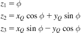
Keywords
Direct kinematics; inverse kinematics; homogeneous transformation; nonholonomic constraints; differential drive WMR; car-like WMR; chain model; Brockett integrator model; omnidirectional WMR; mecanum omnidirectional WMR
2.1 Introduction
Robot kinematics deals with the configuration of robots in their workspace, the relations between their geometric parameters, and the constraints imposed in their trajectories. The kinematic equations depend on the geometrical structure of the robot. For example, a fixed robot can have a Cartesian, cylindrical, spherical, or articulated structure, and a mobile robot may have one two, three, or more wheels with or without constraints in their motion [1–20]. The study of kinematics is a fundamental prerequisite for the study of dynamics, the stability features, and the control of the robot. The development of new and specialized robotic kinematic structures is still a topic of ongoing research, toward the end of constructing robots that can perform more sophisticated and complex tasks in industrial and societal applications [1–20].
The objectives of this chapter are as follows:
• To present the fundamental analytical concepts required for the study of mobile robot kinematics
• To present the kinematic models of nonholonomic mobile robots (unicycle, differential drive, tricycle, and car-like wheeled mobile robots (WMRs))
• To present the kinematic models of 3-wheel, 4-wheel, and multiwheel omnidirectional WMRs.
2.2 Background Concepts
As a preparation for the study of mobile robot kinematics the following background concepts are presented:
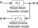
2.2.1 Direct and Inverse Robot Kinematics
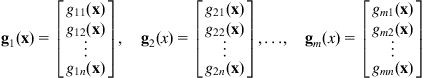
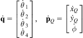
Consider a fixed or mobile robot with generalized coordinates ![]() in the joint (or actuation) space and
in the joint (or actuation) space and ![]() in the task space. Define the vectors:
in the task space. Define the vectors:
 (2.1)
(2.1)
The problem of determining ![]() knowing
knowing ![]() is called the direct kinematics problem. In general
is called the direct kinematics problem. In general ![]() and
and ![]() (
(![]() denotes the n-dimensional Euclidean space) are related by a nonlinear function (model) as:
denotes the n-dimensional Euclidean space) are related by a nonlinear function (model) as:
 (2.2)
(2.2)
The problem of solving Eq. (2.2), that is of finding ![]() from
from ![]() , is called the inverse kinematic problem expressed by:
, is called the inverse kinematic problem expressed by:
![]() (2.3)
(2.3)
The direct and inverse kinematic problems are pictorially shown in Figure 2.1.
In general, kinematics is the branch of mechanics that investigates the motion of material bodies without referring to their masses/moments of inertia and the forces/torques that produce the motion. Clearly, the kinematic equations depend on the fixed geometry of the robot in the fixed world coordinate frame.
To get these motions we must tune appropriately the motions of the joint variables, expressed by the velocities ![]() . We therefore need to find the differential relation of
. We therefore need to find the differential relation of ![]() and
and ![]() . This is called direct differential kinematics and is expressed by:
. This is called direct differential kinematics and is expressed by:
![]() (2.4)
(2.4)
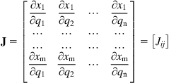
where

and the ![]() matrix:
matrix:
 (2.5)
(2.5)
with ![]() element
element ![]() is called the Jacobian matrix of the robot.1
is called the Jacobian matrix of the robot.1
For each configuration ![]() of the robot, the Jacobian matrix represents the relation of the displacements of the joints with the displacement of the position of the robot in the task space.
of the robot, the Jacobian matrix represents the relation of the displacements of the joints with the displacement of the position of the robot in the task space.
Let ![]() and
and ![]() be the velocities in the joint and task spaces.
be the velocities in the joint and task spaces.
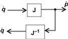
Then, dividing Eq. (2.4) by ![]() we get formally:
we get formally:
![]() (2.6)
(2.6)
Under the assumption that ![]() (
(![]() square) and that the inverse Jacobian matrix
square) and that the inverse Jacobian matrix ![]() exists (i.e., its determinant is not zero:
exists (i.e., its determinant is not zero: ![]() ), from Eq. (2.6) we get:
), from Eq. (2.6) we get:
![]() (2.7)
(2.7)
This is the inverse differential kinematics equation, and is illustrated in Figure 2.2.
Case 1
There are more equations than unknowns ![]() , that is,
, that is, ![]() is overspecified. In this case
is overspecified. In this case ![]() in Eq. (2.7) is replaced by the generalized inverse
in Eq. (2.7) is replaced by the generalized inverse ![]() given by:
given by:
![]() (2.8a)
(2.8a)
under the condition that ![]() is full rank (i.e., rank
is full rank (i.e., rank ![]() =min (m.n)=n) so as
=min (m.n)=n) so as ![]() is invertible. The expression (2.8a) of
is invertible. The expression (2.8a) of ![]() follows by minimizing the squared norm of the difference
follows by minimizing the squared norm of the difference ![]() , that is of the function:
, that is of the function:
![]()
with respect to ![]() . The optimality condition is:
. The optimality condition is:
![]()
which, if solved for ![]() , gives:
, gives:
![]()
Case 2
There are less equations than unknowns ![]() , that is,
, that is, ![]() is underspecified and many choices of
is underspecified and many choices of ![]() lead to the same
lead to the same ![]() . In this case we select
. In this case we select ![]() with the minimum norm, that is, we solve the constrained minimization problem:
with the minimum norm, that is, we solve the constrained minimization problem:
![]()
Introducing the Lagrange multiplier vector ![]() , we get the augmented (unconstrained) Lagrangian minimization problem:
, we get the augmented (unconstrained) Lagrangian minimization problem:
![]()
The optimality conditions are:
![]()
Solving the first for ![]() we get
we get ![]() .
.
Introducing this result into ![]() yields:
yields:
![]()
Therefore, finally we find:
![]()
where
![]() (2.8b)
(2.8b)
under the condition that rank ![]() (i.e.,
(i.e., ![]() invertible). Therefore, when
invertible). Therefore, when ![]() the generalized inverse Eq. (2.8b) should be used.
the generalized inverse Eq. (2.8b) should be used.
Formally, the generalized inverse ![]() of a
of a ![]() real matrix
real matrix ![]() is defined to be the unique
is defined to be the unique ![]() real matrix that satisfies the following four conditions:
real matrix that satisfies the following four conditions:
![]()
![]()
It follows that ![]() has the properties:
has the properties:
![]()
All the above relations are useful when dealing with overspecified or underspecified linear algebraic systems (encountered, e.g., in underactuated or overactuated mechanical systems).
2.2.2 Homogeneous Transformations
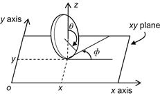
The position and orientation of a solid body (e.g., a robotic link) with respect to the fixed world coordinate frame Oxyz (Figure 2.3) are given by a ![]() transformation matrix
transformation matrix ![]() , called homogeneous transformation, of the type:
, called homogeneous transformation, of the type:
![]() (2.9)
(2.9)
where ![]() is the position vector of the center of gravity
is the position vector of the center of gravity ![]() (or some other fixed point of the link) with respect to Oxyz, and
(or some other fixed point of the link) with respect to Oxyz, and ![]() is a
is a ![]() matrix defined as:
matrix defined as:
![]() (2.10)
(2.10)
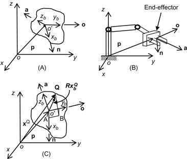
Figure 2.3 (A) Position and orientation of a solid body, (B) position and orientation of a robotic end-effector (a=approach vector, n=normal vector, o=orientation or sliding vector), and (C) position vectors of a point ![]() with respect to the frames Oxyz and
with respect to the frames Oxyz and ![]() .
.
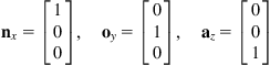
In Eq. (2.10), ![]() ,
, ![]() and
and ![]() are the unit vectors along the axes
are the unit vectors along the axes ![]() ,
, ![]() ,
, ![]() of the local coordinate frame
of the local coordinate frame ![]() . The matrix
. The matrix ![]() represents the rotation of
represents the rotation of ![]() with respect to the reference (world) frame Oxyz. The columns
with respect to the reference (world) frame Oxyz. The columns ![]() ,
, ![]() , and
, and ![]() of
of ![]() are pairwise orthonormal, that is,
are pairwise orthonormal, that is, ![]() where
where ![]() denotes the transpose (row) vector of the column vector
denotes the transpose (row) vector of the column vector ![]() , and
, and ![]() denotes the Euclidean norm of
denotes the Euclidean norm of ![]()
![]() , with
, with ![]() ,
, ![]() , and
, and ![]() being the
being the ![]() components of
components of ![]() , respectively.
, respectively.
Thus the rotation matrix ![]() is orthonormal, that is:
is orthonormal, that is:
![]() (2.11)
(2.11)
To work with homogeneous matrices we use 4-dimensional vectors (called homogeneous vectors) of the type:
 (2.12)
Suppose that ![]() and
and ![]() are the homogeneous position vectors of a point
are the homogeneous position vectors of a point ![]() in the coordinate frames
in the coordinate frames ![]() and Oxyz, respectively. Then, from Figure 2.3C we obtain the following vectorial equation:
and Oxyz, respectively. Then, from Figure 2.3C we obtain the following vectorial equation:
![]()
where
![]()
Thus:
 (2.13a)
or
![]() (2.13b)
(2.13b)
where ![]() is given by Eqs. (2.9) and (2.10). Equation (2.13b) indicates that the homogeneous matrix
is given by Eqs. (2.9) and (2.10). Equation (2.13b) indicates that the homogeneous matrix ![]() contains both the position and orientation of the local coordinate frame
contains both the position and orientation of the local coordinate frame ![]() with respect to the world coordinate frame Oxyz.
with respect to the world coordinate frame Oxyz.
It is easy to verify that:
![]() (2.14)
(2.14)
Indeed, from Eq. (2.13a) we have: ![]() , which by Eq. (2.11) gives:
, which by Eq. (2.11) gives:
![]()
The columns ![]() ,
, ![]() , and
, and ![]() of
of ![]() consist of the direction cosines with respect to Oxyz. Thus the rotation matrices with respect to axes
consist of the direction cosines with respect to Oxyz. Thus the rotation matrices with respect to axes ![]() which are represented as:
which are represented as:
are given by:
 (2.15a)
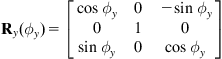 (2.15b)
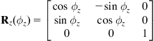 (2.15c)
where ![]() ,
, ![]() , and
, and ![]() are the rotation angles with respect to
are the rotation angles with respect to ![]() ,
, ![]() , and
, and ![]() , respectively.
, respectively.
In mobile robots moving on a horizontal plane, the robot is rotating only with respect to the vertical axis ![]() , and so Eq. (2.15c) is used. Thus, for convenience, we drop the index
, and so Eq. (2.15c) is used. Thus, for convenience, we drop the index ![]() .
.
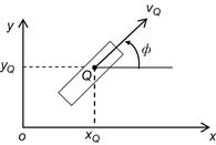
For better understanding, the upper left block of Eq. (2.15c) is obtained directly using the Oxy plane geometry shown in Figure 2.4.

Let a point ![]() in the coordinate frame Oxy, which is rotated about the axis Oz by the angle
in the coordinate frame Oxy, which is rotated about the axis Oz by the angle ![]() . The coordinates of
. The coordinates of ![]() in the frame
in the frame ![]() are
are ![]() and
and ![]() as shown in Figure 2.4. From this figure we see that:
as shown in Figure 2.4. From this figure we see that:
![]() (2.16)
(2.16)
![]() (2.17)
(2.17)
Similarly, one can derive the respective ![]() blocks
blocks ![]() and
and ![]() for the rotations about the
for the rotations about the ![]() and
and ![]() axes, respectively.
axes, respectively.
Given an open kinematic chain of ![]() links, the homogeneous vector
links, the homogeneous vector ![]() of the local coordinate frame
of the local coordinate frame ![]() of the nth link, expressed in the world coordinate frame Oxyz can be found by successive application of Eq. (2.13b), that is, as:
of the nth link, expressed in the world coordinate frame Oxyz can be found by successive application of Eq. (2.13b), that is, as:
![]() (2.18)
(2.18)
where ![]() is the
is the ![]() homogeneous transformation matrix that leads from the coordinate frame of link
homogeneous transformation matrix that leads from the coordinate frame of link ![]() to that of link
to that of link ![]() . The matrices
. The matrices ![]() can be computed by the so-called Denavit–Hartenberg (D–H) method (Section 10.2.1). The general relation (2.18) is of the form (2.2), and provides the robot Jacobian as indicated in Eq. (2.5).
can be computed by the so-called Denavit–Hartenberg (D–H) method (Section 10.2.1). The general relation (2.18) is of the form (2.2), and provides the robot Jacobian as indicated in Eq. (2.5).
2.2.3 Nonholonomic Constraints
A nonholonomic constraint (relation) is defined to be a constraint that contains time derivatives of generalized coordinates (variables) of a system and is not integrable. To understand what this means we first define a holonomic constraint as any constraint which can be expressed in the form:
![]() (2.19)
(2.19)
where ![]() is the vector of generalized coordinates.
is the vector of generalized coordinates.
Now, suppose we have a constraint of the form:
![]() (2.20)
(2.20)
If this constraint can be converted to the form:
![]() (2.21)
(2.21)
we say that it is integrable. Therefore, although ![]() in Eq. (2.20) contains the time derivatives
in Eq. (2.20) contains the time derivatives ![]() , it can be expressed in the holonomic form Eq. (2.21), and so it is actually a holonomic constraint. More specifically we have the following definition.
, it can be expressed in the holonomic form Eq. (2.21), and so it is actually a holonomic constraint. More specifically we have the following definition.
Typical systems that are subject to nonholonomic constraints (and hence are called nonholonomic systems) are underactuated robots, WMRs, autonomous underwater vehicles (AUVs), and unmanned aerial vehicles (UAVs). It is emphasized that “holonomic” does not necessarily mean unconstrained. Surely, a mobile robot with no constraint is holonomic. But a mobile robot capable of only translations is also holonomic.
Nonholonomicity occurs in several ways. For example a robot has only a few motors, say ![]() , where
, where ![]() is the number of degrees of freedom, or the robot has redundant degrees of freedom. The robot can produce at most
is the number of degrees of freedom, or the robot has redundant degrees of freedom. The robot can produce at most ![]() independent motions. The difference
independent motions. The difference ![]() indicates the existence of nonholomicity. For example, a differential drive WMR has two controls (the torques of the two wheel motors), that is,
indicates the existence of nonholomicity. For example, a differential drive WMR has two controls (the torques of the two wheel motors), that is, ![]() , and three degrees of freedom, that is,
, and three degrees of freedom, that is, ![]() . Therefore, it has one
. Therefore, it has one ![]() nonholonomic constraint.
nonholonomic constraint.
Definition 2.2
(Pfaffian constraints)
A nonholonomic constraint is called a Pfaffian constraint if it is linear in ![]() , that is, if it can be expressed in the form:
, that is, if it can be expressed in the form:
![]()
where ![]() are linearly independent row vectors and
are linearly independent row vectors and ![]() .
.
In compact matrix form the above ![]() Pfaffian constraints can be written as:
Pfaffian constraints can be written as:
 (2.22)
An example of integrable Pfaffian constraint is:
![]() (2.23)
(2.23)
This is integrable because it can be derived via differentiation, with respect to time, of the equation of a sphere:
![]()
with constant radius ![]() . The particular resulting sphere by integrating Eq. (2.23) depends on the initial state
. The particular resulting sphere by integrating Eq. (2.23) depends on the initial state ![]() . The collection of all concentric spheres with center at the origin and radius “
. The collection of all concentric spheres with center at the origin and radius “![]() ” is called a foliation with spherical leaves. For example, if
” is called a foliation with spherical leaves. For example, if ![]() the foliation produces a maximal integral manifold
the foliation produces a maximal integral manifold ![]() :
:
![]()
The nonholonomic constraint encountered in mobile robotics is the motion constraint of a disk that rolls on a plane without slipping (Figure 2.5). The no-slipping condition does not allow the generalized velocities ![]() , and
, and ![]() to take arbitrary values.
to take arbitrary values.
Let ![]() be the disk radius. Due to the no-slipping condition the generalized coordinates are constrained by the following equations:
be the disk radius. Due to the no-slipping condition the generalized coordinates are constrained by the following equations:
![]() (2.24)
(2.24)
which are not integrable. These constraints express the condition that the velocity vector of the disk center lies in the midplane of the disk. Eliminating the velocity ![]() in Eq. (2.24) gives:
in Eq. (2.24) gives:
![]()
or
![]() (2.25)
(2.25)
This is the nonholonomic constraint of the motion of the disk. Because of the kinematic constraints (2.24), the disk can attain any final configuration ![]() starting from any initial configuration
starting from any initial configuration ![]() . This can be done in two steps as follows:
. This can be done in two steps as follows:
Given a kinematic constraint one has to determine whether it is integrable or not. This can be done via the Frobenius theorem which uses the differential geometry concepts of distributions and Lie Brackets. We will come to this later (Section 6.2.1).
Two other systems that are subject to nonholonomic constraints are the rolling ball on a plane without spinning on place, and the flying airplane that cannot instantaneously stop in the air or move backward.
2.3 Nonholonomic Mobile Robots
The kinematic models of the following nonholonomic WMRs will be derived:
2.3.1 Unicycle
Unicycle has a kinematic model which is used as a basis for many types of nonholonomic WMRs. For this reason this model has attracted much theoretical attention by WMR controlists and nonlinear systems workers.
Unicycle is a conventional wheel rolling on a horizontal plane, while keeping its body vertical (Figure 2.5). The unicycle configuration (as seen from the bottom via a glass floor) is shown in Figure 2.6.
Its configuration is described by a vector of generalized coordinates: ![]() , that is, the position coordinates of the point of contact
, that is, the position coordinates of the point of contact ![]() with the ground in the fixed coordinate frame Oxy, and its orientation angle
with the ground in the fixed coordinate frame Oxy, and its orientation angle ![]() with respect to the
with respect to the ![]() axis. The linear velocity of the wheel is
axis. The linear velocity of the wheel is ![]() and its angular velocity about its instantaneous rotational axis is
and its angular velocity about its instantaneous rotational axis is ![]() . From Figure 2.6, we find:
. From Figure 2.6, we find:
![]() (2.26)
(2.26)
Eliminating ![]() from the first two equations (2.26) we find the nonholonomic constraint (2.25):
from the first two equations (2.26) we find the nonholonomic constraint (2.25):
![]() (2.27)
(2.27)
Using the notation ![]() and
and ![]() , for simplicity, the kinematic model (2.26) of the unicycle can be written as:
, for simplicity, the kinematic model (2.26) of the unicycle can be written as:
 (2.28a)
or
![]() (2.28b)
(2.28b)
where ![]() is the system Jacobian matrix:
is the system Jacobian matrix:
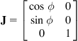 (2.28c)
The linear velocity ![]() and the angular velocity
and the angular velocity ![]() are assumed to be the action (joint) variables of the system.
are assumed to be the action (joint) variables of the system.
The model (2.28a) belongs to the special class of nonlinear systems, called affine systems, and described by a dynamic equation of the form (Chapter 6):
![]() (2.29a)
(2.29a)
![]() (2.29b)
(2.29b)
where ![]() appear linearly, and:
appear linearly, and:
![]()
![]() (2.30)
(2.30)
If ![]() the system has a less number of actuation variables (controls) than the degrees of freedom under control and is known as underactuated system. If
the system has a less number of actuation variables (controls) than the degrees of freedom under control and is known as underactuated system. If ![]() we have an overactuated system. In practice, usually
we have an overactuated system. In practice, usually ![]() . The vector
. The vector ![]() is actually the state vector of the system and
is actually the state vector of the system and ![]() the control vector. The term
the control vector. The term ![]() is called “drift,” and the system with
is called “drift,” and the system with ![]() is called a “driftless” system. The column vector set:
is called a “driftless” system. The column vector set:
 (2.31)
is referred to as the system’s vector field. It is assumed that the set ![]() contains at least an open set that involves the origin of
contains at least an open set that involves the origin of ![]() . If
. If ![]() does not contain the origin, then the system is not “driftless.”
does not contain the origin, then the system is not “driftless.”
The unicycle model (2.28a) is a 2-input driftless affine system with two vector fields:
 (2.32)
The Jacobian formulation (2.28c) organizes the two column vector fields into a matrix ![]() . Each action variable
. Each action variable ![]() in Eq. (2.29a) is actually a coefficient that determines how much of
in Eq. (2.29a) is actually a coefficient that determines how much of ![]() is contributing into the result
is contributing into the result ![]() . The vector field
. The vector field ![]() of the unicycle allows pure translation, and the field
of the unicycle allows pure translation, and the field ![]() allows pure rotation.
allows pure rotation.
2.3.2 Differential Drive WMR
Indoor and other mobile robots use the differential drive locomotion type (Figure 1.20). The Pioneer WMR shown in Figure 1.11 is an example of differential drive WMR. The geometry and kinematic parameters of this robot are shown in Figure 2.7. The pose (position/orientation) vector of the WMR and its speed are respectively:
 (2.33)
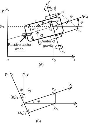
Figure 2.7 (A) Geometry of differential drive WMR, (B) Diagram illustrating the nonholonomic constraint.
The angular positions and speeds of the left and right wheels are ![]() , respectively.
, respectively.
The following assumptions are made:
• Wheels are rolling without slippage
• The guidance (steering) axis is perpendicular to the plane Oxy
• The point ![]() coincides with the center of gravity
coincides with the center of gravity ![]() , that is,
, that is, ![]() .2
.2
Let ![]() and
and ![]() be the linear velocity of the left and right wheel respectively, and
be the linear velocity of the left and right wheel respectively, and ![]() the velocity of the wheel midpoint
the velocity of the wheel midpoint ![]() of the WMR. Then, from Figure 2.7A we get:
of the WMR. Then, from Figure 2.7A we get:
![]() (2.34a)
(2.34a)
Adding and subtracting ![]() and vl we get
and vl we get
![]() (2.34b)
(2.34b)
where, due to the nonslippage assumption, we have ![]() and
and ![]() . As in the unicycle case
. As in the unicycle case ![]() and
and ![]() are given by:
are given by:
![]() (2.35)
(2.35)
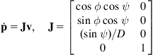
and so the kinematic model of this WMR is described by the following relations:
![]() (2.36a)
(2.36a)
![]() (2.36b)
(2.36b)
![]() (2.36c)
(2.36c)
Analogously to Eq. (2.28a,b) the kinematic model (2.36a–c) can be written in the driftless affine form:
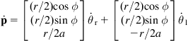 (2.37a)
![]() (2.37b)
(2.37b)
where
 (2.37c)
and ![]() is the WMR’s Jacobian:
is the WMR’s Jacobian:
 (2.37d)
Here, the two 3-dimensional vector fields are:
 (2.38)
The field ![]() allows the rotation of the right wheel, and
allows the rotation of the right wheel, and ![]() allows the rotation of the left wheel. Eliminating
allows the rotation of the left wheel. Eliminating ![]() in Eq. (2.35) we get as usual the nonholonomic constraint (2.25) or (2.27).
in Eq. (2.35) we get as usual the nonholonomic constraint (2.25) or (2.27).
![]() (2.39)
(2.39)
which expresses the fact that the point ![]() is moving along
is moving along ![]() , and its velocity along the axis
, and its velocity along the axis ![]() is zero (no lateral motion), that is (Figure 2.7B):
is zero (no lateral motion), that is (Figure 2.7B):
![]()
where ![]() and
and ![]() .
.
The Jacobian matrix ![]() in Eq. (2.37d) has three rows and two columns, and so it is not invertible. Therefore, the solution of Eq. (2.37b) for
in Eq. (2.37d) has three rows and two columns, and so it is not invertible. Therefore, the solution of Eq. (2.37b) for ![]() is given by:
is given by:
![]() (2.40)
(2.40)
where ![]() is the generalized inverse of
is the generalized inverse of ![]() given by Eq. (2.8a). However, here
given by Eq. (2.8a). However, here ![]() can be computed directly by using Eq. (2.34a), and observing from Figure 2.7B that:
can be computed directly by using Eq. (2.34a), and observing from Figure 2.7B that:
![]()
Thus, using this equation in Eq. (2.34a) we obtain:
![]() (2.41a)
(2.41a)
that is:
or
![]() (2.41b)
(2.41b)
where3 :
![]() (2.41c)
(2.41c)
The nonholonomic constraint (2.39) can be written as:
![]() (2.42)
(2.42)
Clearly, if ![]() , then the difference between
, then the difference between ![]() and
and ![]() determines the robot’s rotation speed
determines the robot’s rotation speed ![]() and its direction. The instantaneous curvature radius
and its direction. The instantaneous curvature radius ![]() is given by (Eq. 1.1):
is given by (Eq. 1.1):
![]() (2.43a)
(2.43a)
and the instantaneous curvature coefficient is:
![]() (2.43b)
(2.43b)
Example 2.1
Derive the kinematic relations (2.35) using the rotation matrix concept (2.17).
Solution
Here, the point ![]() of Figure 2.4 is the point
of Figure 2.4 is the point ![]() in Figure 2.7. The WMR velocities along the local coordinate axes
in Figure 2.7. The WMR velocities along the local coordinate axes ![]() and
and ![]() are
are ![]() and
and ![]() . The corresponding velocities in the world coordinate frame are
. The corresponding velocities in the world coordinate frame are ![]() and
and ![]() . Therefore, for a given
. Therefore, for a given ![]() , (2.17) gives:
, (2.17) gives:
![]() (2.44)
(2.44)
Now, the condition of no lateral wheel movement implies that
![]()
and ![]() . Therefore, the above relation gives:
. Therefore, the above relation gives:
![]()
as desired.
Example 2.2
Derive the kinematic equations and constraints of a differential drive WMR by relaxing the no-slipping condition of the wheels’ motion.
Solution
We will work with the WMR of Figure 2.7. Considering the rotation about the center of gravity ![]() we get the following relations:
we get the following relations:
![]()
![]()
Therefore, the kinematic equations (2.41a) and the nonholonomic constraint (2.42) become:
![]()
![]()
![]()
Now, assume that the wheels are subject to longitudinal and lateral slip [10]. To include the slip into the kinematics of the robot, we introduce two variables ![]() ,
, ![]() for the longitudinal slip displacements of the right wheel and left wheel, respectively, and two variables
for the longitudinal slip displacements of the right wheel and left wheel, respectively, and two variables ![]() ,
, ![]() for the corresponding lateral slip displacements. Thus, here:
for the corresponding lateral slip displacements. Thus, here:
![]()
The slipping wheels’ velocities are now given by:
![]()
where ![]() and
and ![]() are the steering angles of the wheels.
are the steering angles of the wheels.
Using these relations for ![]() and
and ![]() the above kinematic equations are written as:
the above kinematic equations are written as:
![]()
![]()
and the nonholonomic constraint becomes:
![]()
![]()
In our WMR the two wheels have a common axis and are unsteered. Therefore, ![]() . For WMRs with steered wheels we may have
. For WMRs with steered wheels we may have ![]() ,
, ![]() . In our case
. In our case ![]() , and so the two kinematic equations, solved for the angular wheel velocities
, and so the two kinematic equations, solved for the angular wheel velocities ![]() and
and ![]() , give:
, give:
![]()
where the inverse Jacobian is:
![]()
The nonholonomic constraints are written in Pfaffian form:
![]()
where
![]()
![]()
In the special case where only lateral slip takes place (i.e., ![]() ,
, ![]() ), the components
), the components ![]() and
and ![]() are dropped from
are dropped from ![]() , and the matrices
, and the matrices ![]() and
and ![]() are reduced appropriately, having only five columns. Note that here the wheels are fixed and so
are reduced appropriately, having only five columns. Note that here the wheels are fixed and so ![]() where
where ![]() is the lateral slipping velocity of the body of the WMR. Typically, the slipping variables, which are unknown and nonmeasurable are treated as disturbances via disturbance rejection and robust control techniques.
is the lateral slipping velocity of the body of the WMR. Typically, the slipping variables, which are unknown and nonmeasurable are treated as disturbances via disturbance rejection and robust control techniques.
2.3.3 Tricycle
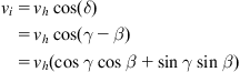
The motion of this WMR is controlled by the wheel steering angular velocity ![]() and its linear velocity
and its linear velocity ![]() (or its angular velocity
(or its angular velocity ![]() , where
, where ![]() is the radius of the wheel) (Figure 2.8).
is the radius of the wheel) (Figure 2.8).
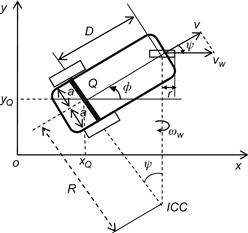
The orientation angle and angular velocity are ![]() and
and ![]() , respectively. It is assumed that the vehicle has its guidance point
, respectively. It is assumed that the vehicle has its guidance point ![]() in the back of the powered wheel (i.e., it has a central back axis). The state of the robot’s motion is:
in the back of the powered wheel (i.e., it has a central back axis). The state of the robot’s motion is:
![]()
Using the above relations we find:
 (2.45)
where ![]() is the vector of joint velocities (control variables), and
is the vector of joint velocities (control variables), and
 (2.46)
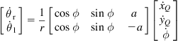
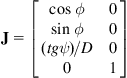
is the Jacobian matrix. This Jacobian is again noninvertible, but we can find the inverse kinematic equations directly using the relations:
![]() (2.47a)
(2.47a)
and
![]() (2.47b)
(2.47b)
The instantaneous curvature radius ![]() is given by (Figure 2.8):
is given by (Figure 2.8):
![]() (2.48)
(2.48)
From Eq. (2.45) we see that the tricycle is again a 2-input driftless affine system with vector fields:

that allow steering wheel motion ![]() , and steering angle motion
, and steering angle motion ![]() , respectively.
, respectively.
2.3.4 Car-Like WMR
The geometry of the car-like mobile robot is shown in Figure 2.9A and the A.W.E.S.O.M.-9000 line-tracking car-like robot prototype (Aalborg University) in Figure 2.9B.
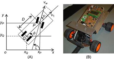
Figure 2.9 (A) Kinematic structure of a car-like robot, (B) A car-like robot prototype. Source: http://sqrt-1.dk/robot/robot.php
The state of the robot’s motion is represented by the vector [20]:
![]() (2.49)
(2.49)
where ![]() ,
, ![]() are the Cartesian coordinates of the wheel axis midpoint
are the Cartesian coordinates of the wheel axis midpoint ![]() ,
, ![]() is the orientation angle of the vehicle, and
is the orientation angle of the vehicle, and ![]() is the steering angle. Here, we have two nonholonomic constraints, one for each wheel pair, that is:
is the steering angle. Here, we have two nonholonomic constraints, one for each wheel pair, that is:
![]() (2.50a)
(2.50a)
![]() (2.50b)
(2.50b)
where ![]() and
and ![]() are the position coordinates of the front wheels midpoint
are the position coordinates of the front wheels midpoint ![]() . From Figure 2.9 we get:
. From Figure 2.9 we get:
![]()
Using these relations the second kinematic constraint (2.50b) becomes:
![]()
The two nonholonomic constraints are written in the matrix form:
![]() (2.51a)
(2.51a)
where
![]() (2.51b)
(2.51b)
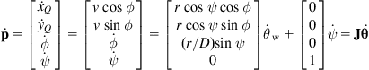
The kinematic equations for a rear-wheel driving car are found to be (Figure 2.9):
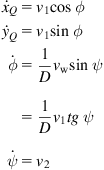 (2.52)
These equations can be written in the affine form:
 (2.53)
that has the vector fields:

allowing the driving motion ![]() and the steering motion
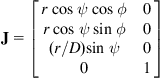
and the steering motion ![]() , respectively. The Jacobian form of Eq. (2.53) is:
, respectively. The Jacobian form of Eq. (2.53) is:
![]() (2.54)
(2.54)
with Jacobian matrix:
 (2.55)
Here, there is a singularity at ![]() , which corresponds to the “jamming” of the WMR when the front wheels are normal to the longitudinal axis of its body. Actually, this singularity does not occur in practice due to the restricted range of the steering angle
, which corresponds to the “jamming” of the WMR when the front wheels are normal to the longitudinal axis of its body. Actually, this singularity does not occur in practice due to the restricted range of the steering angle ![]() .
.
The kinematic model for the front wheel driving vehicle is Eqs. 2.45 and (2.46) [20]:
 (2.56a)
In this case the previous singularity does not occur, since at ![]() the car can still (in principle) pivot about its rear wheels. Using the new inputs
the car can still (in principle) pivot about its rear wheels. Using the new inputs ![]() and
and ![]() defined as:
defined as:
![]()
the above model is transformed to:
 (2.56b)
where ![]() is the total steering angle with respect to the axis Ox.
is the total steering angle with respect to the axis Ox.
Indeed, from ![]() and
and ![]() (Figure 2.9), and Eq. (2.56a) we get:
(Figure 2.9), and Eq. (2.56a) we get:
![]()
![]()
![]()
![]()
We observe, from Eq. (2.56b), that the kinematic model for ![]() ,
, ![]() , and
, and ![]() (i.e., the first, second, and fourth equation in Eq. (2.56b)) is actually a unicycle model (2.28a).
(i.e., the first, second, and fourth equation in Eq. (2.56b)) is actually a unicycle model (2.28a).
Two special cases of the above car-like model are known as:
The Reeds-Shepp car is obtained by restricting the values of the velocity ![]() to three distinct values
to three distinct values ![]() ,
, ![]() , and
, and ![]() . These values appear to correspond to three distinct “gears”: “forward,” “park,” or “reverse.” The Dubins car is obtained when the reverse motion is not allowed in the Reeds-Shepp car, that is, the value
. These values appear to correspond to three distinct “gears”: “forward,” “park,” or “reverse.” The Dubins car is obtained when the reverse motion is not allowed in the Reeds-Shepp car, that is, the value ![]() is excluded, in which case
is excluded, in which case ![]() .
.
Example 2.3
It is desired to find the steering angle ![]() which is required for a rear-wheel driven car-like WMR to go from its present position
which is required for a rear-wheel driven car-like WMR to go from its present position ![]() to a given goal
to a given goal ![]() . The available data, which are obtained via proper sensors, are the distance
. The available data, which are obtained via proper sensors, are the distance ![]() between
between ![]() and
and ![]() and the angle
and the angle ![]() of the vector
of the vector ![]() with respect to the current vehicle orientation.
with respect to the current vehicle orientation.
Solution
We will work with the geometry of Figure 2.10 [19]. The kinematic equations of the WMR are given by Eq. (2.52). The WMR will go from the position ![]() to the goal
to the goal ![]() following a circular path with curvature:
following a circular path with curvature:
![]()
determined using the bicycle equivalent model, that combines the two front wheels and the two rear wheels (Figure 2.10, left).
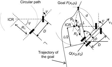
On the other hand, the curvature ![]() of the circular path that passes through the goal, is obtained from the relation (Figure 2.10, right):
of the circular path that passes through the goal, is obtained from the relation (Figure 2.10, right):
![]()
that is:
![]() (2.57a)
(2.57a)
To meet the goal tracking requirement the above two curvatures ![]() and
and ![]() must be the same, that is:
must be the same, that is:
![]()
Therefore:
![]() (2.57b)
(2.57b)
Equation (2.57b) gives the steering angle ![]() in terms of the data
in terms of the data ![]() and
and ![]() , and can be used to pursuit tracking of goals (targets) that are moving along given trajectories. In these cases the goal
, and can be used to pursuit tracking of goals (targets) that are moving along given trajectories. In these cases the goal ![]() lies at the intersection of the goal trajectory and the look-ahead circle. To get a better interpretation of (2.57a), we use the lateral distance
lies at the intersection of the goal trajectory and the look-ahead circle. To get a better interpretation of (2.57a), we use the lateral distance ![]() between the vehicles orientation (heading) vector and the goal point, which is given by (Figure 2.10):
between the vehicles orientation (heading) vector and the goal point, which is given by (Figure 2.10):
![]()
Then, the curvature ![]() in Eq. (2.57a) is given by:
in Eq. (2.57a) is given by:
![]()
This indicates that the curvature ![]() of the path resulting from the steering angle
of the path resulting from the steering angle ![]() should be:
should be:
![]() (2.57c)
(2.57c)
Equation (2.57c) is a “proportional control law” and shows that the curvature ![]() of the robot’s path should be proportional to the cross track error
of the robot’s path should be proportional to the cross track error ![]() some look-ahead distance in front of the WMR with a gain
some look-ahead distance in front of the WMR with a gain ![]() .
.
2.3.5 Chain and Brockett—Integrator Models
The general 2-input n-dimensional chain model (briefly ![]() -chain model) is:
-chain model) is:
 (2.58)
The Brockett (single) integrator model is:
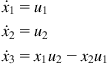 (2.59)
and the double integrator model is:
 (2.60)
The nonholonomic WMR kinematic models can be transformed to the above models. Here, the unicycle model (which also covers the differential drive model) and the car-like model will be considered.
2.3.5.1 Unicycle WMR
The unicycle kinematic model is given by Eq. (2.26):
![]() (2.61)
(2.61)
Using the transformation:
 (2.62)
the unicycle model is converted to the (2,3)-chain form:
 (2.63)
where ![]() and
and ![]() .
.
Defining new state variables:
![]() (2.64)
(2.64)
the (2,3)-chain model is converted to the Brockett integrator:
 (2.65)
2.3.5.2 Rear-Wheel Driving Car
The rear-wheel driven car model is given by Eq. (2.52):
![]() (2.66)
(2.66)
Using the state transformation:
![]() (2.67)
(2.67)
and input transformation:
![]() (2.68)
(2.68)
![]()
for ![]() and
and ![]() , the model (2.66) is converted to the (2,4)-chain form:
, the model (2.66) is converted to the (2,4)-chain form:
 (2.69)
2.3.6 Car-Pulling Trailer WMR
This is an extension of the car-like WMR, where ![]() one-axis trailers are attached to a car-like robot with rear-wheel drive. This type of trailer is used, for example, at airports for transporting luggage. The form of equations depend crucially on the exact point at which the trailer is attached and on the choice of body frames. Here, for simplicity each trailer will be assumed to be connected to the axle midpoint of the previous trailer (zero hooking) as shown in Figure 2.11 [20].
one-axis trailers are attached to a car-like robot with rear-wheel drive. This type of trailer is used, for example, at airports for transporting luggage. The form of equations depend crucially on the exact point at which the trailer is attached and on the choice of body frames. Here, for simplicity each trailer will be assumed to be connected to the axle midpoint of the previous trailer (zero hooking) as shown in Figure 2.11 [20].
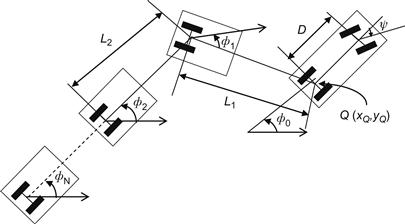
The new parameter introduced here is the distance from the center of the back axle of trailer ![]() to the point at which is hitched to the next body. This is called the hitch (or hinge-to-hinge) length denoted by
to the point at which is hitched to the next body. This is called the hitch (or hinge-to-hinge) length denoted by ![]() . The car length is
. The car length is ![]() . Let
. Let ![]() be the orientation of the ith trailer, expressed with respect to the world coordinate frame. Then from the geometry of Figure 2.11 we get the following equations:
be the orientation of the ith trailer, expressed with respect to the world coordinate frame. Then from the geometry of Figure 2.11 we get the following equations:

which give the following nonholonomic constraints:
![]()
![]()
![]()
for ![]() .
.
In analogy to Eq. (2.52) the kinematic equations of the N-trailer are found to be:
 (2.70)
which, obviously, represent a driftless affine system with two inputs ![]() and
and ![]() , states:
, states:
![]()
We observe that the first four lines of the fields ![]() and
and ![]() represent the (powered) car-like WMR itself.
represent the (powered) car-like WMR itself.
2.4 Omnidirectional WMR Kinematic Modeling
The following WMRs will be considered [2,4,11,12,16]:
• Multiwheel omnidirectional WMR with orthogonal (universal) wheels
• Four-wheel omnidirectional WMR with mecanum wheels that have a roller angle ![]() .
.
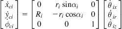
2.4.1 Universal Multiwheel Omnidirectional WMR
The geometric structure of a multiwheel omnirobot is shown in Figure 2.12A. Each wheel has three velocity components [16]:
• Its own velocity ![]() , where
, where ![]() is the common wheel radius and
is the common wheel radius and ![]() its own angular velocity
its own angular velocity
• An induced velocity ![]() which is due to the free rollers (here assumed of the universal type; roller angle
which is due to the free rollers (here assumed of the universal type; roller angle ![]() )
)
• A velocity component ![]() which is due to the rotation of the robotic platform about its center of gravity
which is due to the rotation of the robotic platform about its center of gravity ![]() , that is,
, that is, ![]() , where
, where ![]() is the angular velocity of the platform and
is the angular velocity of the platform and ![]() is the distance of the wheel from
is the distance of the wheel from ![]() .
.

Figure 2.12 (A) Velocity vector of wheel ![]() . The velocity
. The velocity ![]() is the robot vehicle velocity due to the wheel motion, (B) An example of a 3-wheel setup. Source: http://deviceguru.com/files/rovio-3.jpg.
is the robot vehicle velocity due to the wheel motion, (B) An example of a 3-wheel setup. Source: http://deviceguru.com/files/rovio-3.jpg.
Here, the roller angle is ![]() , and so:
, and so:
![]() (2.71a)
(2.71a)
 (2.71b)
Thus the total velocity of the wheel ![]() is:
is:
![]() (2.72)
(2.72)
where ![]() and
and ![]() are the
are the ![]() components of vh, that is:
components of vh, that is:
![]()
Equation (2.72) is general and can be used in WMRs with any number of wheels.
Thus, for example, in the case of a 3-wheel robot we may choose the angle ![]() for the wheels 1, 2, and 3 as 0°, 120°, and 240°, respectively, and get the equations:
for the wheels 1, 2, and 3 as 0°, 120°, and 240°, respectively, and get the equations:
![]() (2.73)
(2.73)
with ![]() . Now, defining the vectors:
. Now, defining the vectors:
![]()
we can write Eq. (2.73) in the inverse Jacobian form:
![]() (2.74a)
(2.74a)
where
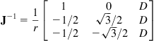 (2.74b)
Here ![]() , and Eq. (2.74a) can be inverted to give
, and Eq. (2.74a) can be inverted to give ![]() .
.
It is remarked that using omniwheels at different angles we can obtain an overall velocity of the WMR’s platform which is greater than the maximum angular velocity of each wheel. For example, selecting in the above 3-wheel case ![]() and
and ![]() we get from Eq. (2.71b):
we get from Eq. (2.71b):
![]()
The ratio ![]() is called the velocity augmentation factor (VAF) [16]:
is called the velocity augmentation factor (VAF) [16]:
![]()
and depends on the number of wheels used and their angular positions on the robot’s body. As a further example, consider a 4-wheel robot with ![]() and
and ![]() . Then, Eq. (2.71b) gives:
. Then, Eq. (2.71b) gives:
![]()
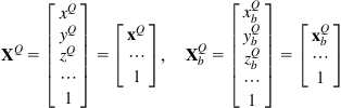
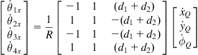
Example 2.4
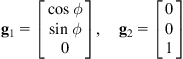
We are given the 4-universal-wheel omnidirectional robot of Figure 2.13, where the angles of the wheels with respect to the axis ![]() of the vehicle’s coordinate frame are
of the vehicle’s coordinate frame are ![]()
![]() . Derive the kinematic equations of the robot in terms of the unit directional vectors
. Derive the kinematic equations of the robot in terms of the unit directional vectors ![]() of the wheel velocities, with respect to the local coordinate frame
of the wheel velocities, with respect to the local coordinate frame ![]() .
.

Solution
Let ![]() be the robot’s angular velocity, and
be the robot’s angular velocity, and ![]() its linear velocity with world-frame coordinates
its linear velocity with world-frame coordinates ![]() and
and ![]() .
.
The unit directional vectors of the wheel velocities are:
![]()
where it was assumed that the axis of wheel 4 coincides with axis Qxr.
The relation between ![]() ,
, ![]() and
and ![]() ,
, ![]() is given by the rotational matrix
is given by the rotational matrix ![]() (Eq. 2.17), that is:
(Eq. 2.17), that is:
![]()
or
![]()
Now, we have:

or, in compact, form:
![]() (2.75a)
(2.75a)
where
 (2.75b)
![]() (2.75c)
(2.75c)
with:
![]() (2.75d)
(2.75d)
As usual, this inverse Jacobian equation gives the required angular wheel speeds ![]()
![]() that lead to the desired linear velocity
that lead to the desired linear velocity ![]() , and angular velocity
, and angular velocity ![]() of the robot. A discussion of the modeling and control problem of a WMR with this structure is provided in Ref. [17].
of the robot. A discussion of the modeling and control problem of a WMR with this structure is provided in Ref. [17].
2.4.2 Four–Wheel Omnidirectional WMR with Mecanum Wheels
Consider the 4-wheel WMR of Figure 2.14, where the mecanum wheels have roller angle ![]() [2,4].
[2,4].

Figure 2.14 Four-mecanum-wheel WMR (A) Kinematic geometry (B) A real 4-mecanum-wheel WMR. Source: http://www.automotto.com/entry/airtrax-wheels-go-in-any-direction.
Here, we have four-wheel coordinate frames ![]() . The angular velocity
. The angular velocity ![]() of the wheel
of the wheel ![]() has three components:
has three components:
The wheel velocity vector ![]() in
in ![]() coordinates is given by:
coordinates is given by:
 (2.76)
for ![]() , where
, where ![]() is the wheel radius,
is the wheel radius, ![]() is the roller radius, and
is the roller radius, and ![]() the roller angle. The robot velocity vector
the roller angle. The robot velocity vector ![]() in the
in the ![]() coordinate frame Eqs. 2.9–(2.13) is:
coordinate frame Eqs. 2.9–(2.13) is:
 (2.77)
where ![]() denotes the rotation angle (orientation) of the frame
denotes the rotation angle (orientation) of the frame ![]() with respect to
with respect to ![]() , and
, and ![]() ,
, ![]() are the translations of
are the translations of ![]() with respect to
with respect to ![]() . Introducing Eq. (2.76) into Eq. (2.77) we get:
. Introducing Eq. (2.76) into Eq. (2.77) we get:
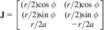
![]() (2.78)
(2.78)
 (2.79)
is the Jacobian matrix of wheel ![]() , which is square and invertible. If all wheels are identical (except for the orientation of the rollers), the kinematic parameters of the robot in the configuration shown in Figure 2.14 are:
, which is square and invertible. If all wheels are identical (except for the orientation of the rollers), the kinematic parameters of the robot in the configuration shown in Figure 2.14 are:
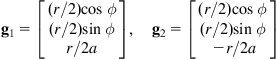
![]()
![]() (2.80)
(2.80)
![]()
Thus, the Jacobian matrices (2.79) are:
 (2.81)
The robot motion is produced by the simultaneous motion of all wheels.
In terms of ![]() (i.e., the wheels’ angular velocities around their axles) the velocity vector
(i.e., the wheels’ angular velocities around their axles) the velocity vector ![]() is given by:
is given by:
 (2.82)
The robot speed vector ![]() in the world coordinate frame is obtained as:
in the world coordinate frame is obtained as:
 (2.83)
where ![]() is the rotation angle of the platform’s coordinate frame
is the rotation angle of the platform’s coordinate frame ![]() around the
around the ![]() axis which is orthogonal to Oxy. Inverting Eqs. (2.82) and (2.83) we get the inverse kinematic model, which gives the angular speeds
axis which is orthogonal to Oxy. Inverting Eqs. (2.82) and (2.83) we get the inverse kinematic model, which gives the angular speeds ![]()
![]() of the wheels around their hubs required to get a desired speed
of the wheels around their hubs required to get a desired speed ![]() of the robot:
of the robot:
 (2.84)
 (2.85)
For historical awareness, we mention here that the mecanum wheel was invented by the Swedish engineer Bengt Ilon in 1973 during his work at the Swedish company Mecanum AB. For this reason it is also known as Ilon wheel or Swedish wheel.
Example 2.5
It is desired to construct a mecanum wheel with ![]() rollers of angle
rollers of angle ![]() . Determine the roller length
. Determine the roller length ![]() and the thickness
and the thickness ![]() of the wheel.
of the wheel.
Solution
We consider the wheel geometry shown in Figure 2.15, where ![]() is the wheel radius [18].
is the wheel radius [18].
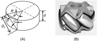
Figure 2.15 (A) Geometry of mecanum wheel where the rollers are assumed to be placed peripherally, (B) A 6-roller wheel example. Source: http://store.kornylak.com/SearchResults.asp?Cat=7.
From this figure we get the following relations:
![]() (2.86a)
(2.86a)
![]() (2.86b)
(2.86b)
![]() (2.86c)
(2.86c)
![]() (2.86d)
(2.86d)
From Eq. (2.86a–c) we have:
![]() (2.87)
(2.87)
whence:
![]() (2.88)
(2.88)
Solving (2.87) for ![]() and noting that
and noting that ![]() , (2.86d) gives:
, (2.86d) gives:
![]() (2.89)
(2.89)
For a roller angle ![]() , Eqs. (2.88) and (2.89) give:
, Eqs. (2.88) and (2.89) give:
![]() (2.90a)
(2.90a)
![]() (2.90b)
(2.90b)
For a roller angle ![]() (universal wheel) we get:
(universal wheel) we get:
![]() (2.91a)
(2.91a)
![]() (2.91b)
(2.91b)
In this case, ![]() can have any convenient value required by other design considerations.
can have any convenient value required by other design considerations.
References
1. Angelo A. Robotics: a reference guide to new technology Boston, MA: Greenwood Press; 2007.
2. Muir PF, Neuman CP. Kinematic modeling of wheeled mobile robots. J Rob Syst. 1987;4(2):281–329.
3. Alexander JC, Maddocks JH. On the kinematics of wheeled mobile robots. Int J Rob Res. 1981;8(5):15–27.
4. Muir PF, Neuman C. Kinematic modeling for feedback control of an omnidirectional wheeled mobile robot. In: Proceedings of IEEE international conference on robotics and automation, Raleigh, NC; 1987, p. 1772–8.
5. Kim DS, Hyun Kwon W, Park HS. Geometric kinematics and applications of a mobile robot. Int J Control Autom Syst. 2003;1(3):376–384.
6. Rajagopalan R. A generic kinematic formulation for wheeled mobile robots. J Rob Syst. 1997;14:77–91.
7. Sreenivasan SV. Kinematic geometry of wheeled vehicle systems. In: Proceedings of 24th ASME mechanism conference, Irvine, CA, 96-DETC-MECH-1137; 1996.
8. Balakrishna R, Ghosal A. Two dimensional wheeled vehicle kinematics. IEEE Trans Rob Autom. 1995;11(1):126–130.
9. Killough SM, Pin FG. Design of an omnidirectional and holonomic wheeled platform design. In: Proceedings of IEEE conference on robotics and automation, Nice, France; 1992, p. 84–90.
10. Sidek N, Sarkar N. Dynamic modeling and control of nonholonomic mobile robot with lateral slip. In: Proceedings of seventh WSEAS international conference on signal processing robotics and automation (ISPRA’08), Cambridge, UK; February 20–22, 2008, p. 66–74.
11. Giovanni I. Swedish wheeled omnidirectional mobile robots: kinematics analysis and control. IEEE Trans Rob. 2009;25(1):164–171.
12. West M, Asada H. Design of a holonomic omnidirectional vehicle. In: Proceedings of IEEE conference on robotics and automation, Nice, France; May 1992, p. 97–103.
13. Chakraborty N, Ghosal A. Kinematics of wheeled mobile robots on uneven terrain. Mech Mach Theory. 2004;39:1273–1287.
14. Sordalen OJ, Egeland O. Exponential stabilization of nonholonomic chained systems. IEEE Trans Autom Control. 1995;40(1):35–49.
15. Khalil H. Nonlinear Systems Upper Saddle River, NJ: Prentice Hall; 2001.
16. Ashmore M, Barnes N. Omni-drive robot motion on curved paths: the fastest path between two points is not a straight line. In: Proceedings of 15th Australian joint conference on artificial intelligence: advances in artificial intelligence (AI’02) London: Springer; 2002; p. 225–36.
17. Huang L, Lim YS, Li D, Teoh CEL. Design and analysis of a four-wheel omnidirectional mobile robot. In: Proceedings of second international conference on autonomous robots and agents, Palmerston North, New Zealand; December 2004. p. 425–8.
18. Doroftei I, Grosu V, Spinu V. Omnidirectional mobile robot: design and implementation. In: Habib MK, ed. Bioinspiration and robotics: walking and climbing robots. Vienna, Austria: I-Tech; 2007;512–527.
19. Phairoh T, Williamson K. Autonomous mobile robots using real time kinematic signal correction and global positioning system control. In: Proceedings of 2008 IAJC-IJME international conference on engineering and technology, Sheraton, Nashville, TN; November 2008, Paper 087/IT304.
20. De Luca A, Oriolo G, Samson C. Feedback control of a nonholonomic car-like robot. In: Laumond J-P, ed. Robot motion planning and control. Berlin, New York: Springer; 1998;171–253.
1It is remarked that in many works the Jacobian matrix is defined as the transpose of that defined in Eq. (2.5).
2In Figure 2.7, the points ![]() and
and ![]() are shown distinct in order to use the same figure in all configurations with
are shown distinct in order to use the same figure in all configurations with ![]() and
and ![]() separated by distance
separated by distance ![]() .
.
3As an exercise, the reader is advised to derive Eq. (2.41c) using Eq. (2.8a).