
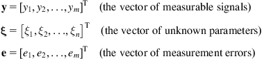
Mobile Robot Dynamics
Mobile robot dynamics is a challenging field on its own, especially due to the variety of the imposed constraints. Delicate stability and control problems that have very often to be faced are due to longitudinal or lateral slip, and to the features of the ground (roughness, etc.). This chapter has the following objectives: (i) to present the general dynamic modeling concepts and techniques of robots, (ii) to study the Newton–Euler and Lagrange dynamic models of differential-drive mobile robots, (iii) to study the dynamics of differential-drive mobile robots with longitudinal and lateral slip, (iv) to derive a dynamic model of car-like wheeled mobile robots, (v) to derive a dynamic model of three-wheel omnidirectional robots, and (vi) to derive a dynamic model of four-wheel mecanum omnidirectional robots.
Keywords
Newton–Euler dynamic model; Lagrange dynamic model; slip dynamic model; force–torque diagram; car-like dynamic model; omnidirectional WMR dynamic model; three-wheel omnidirectional robot; four-wheel omnidirectional robot
3.1 Introduction
The next problem in the study of all types of robots, after kinematics, is the dynamic modeling [1–4]. Dynamic modeling is performed using the laws of mechanics that are based on the three physical elements: inertia, elasticity, and friction that are present in any real mechanical system such as the robot. Mobile robot dynamics is a challenging field on its own and has attracted considerable attention by researchers and engineers over the years. Most mobile robots, employed in practice, use conventional wheels and are subject to nonholonomic constraints that need particular treatment. Delicate stability and control problems, that often have to be faced in the design of a mobile robot, are due to the existence of longitudinal and lateral slip in the movement of the wheeled mobile robot (WMR) wheels [5–7].
This chapter has the following objectives:
• To present the general dynamic modeling concepts and techniques of robots.
• To study the Newton–Euler and Lagrange dynamic models of differential-drive mobile robots.
• To study the dynamics of differential-drive mobile robots with longitudinal and lateral slip.
• To derive a dynamic model of car-like WMRs.
• To derive a dynamic model of three-wheel omnidirectional robots.
• To derive a dynamic model of four-wheel mecanum omnidirectional robots.
3.2 General Robot Dynamic Modeling
Robot dynamic modeling deals with the derivation of the dynamic equations of the robot motion. This can be done using the following two methodologies:
The complexity of the Newton–Euler method is O(n), whereas the complexity of the Lagrange method can only be reduced up to ![]() , where n is the number of degrees of freedom.
, where n is the number of degrees of freedom.
Like kinematics, dynamics is distinguished in:
Direct dynamics provides the dynamic equations that describe the dynamic responses of the robot to given forces/torques ![]() that are exerted by the motors.
that are exerted by the motors.
Inverse dynamics provides the forces/torques that are needed to get desired trajectories of the robot links. Direct and inverse dynamic modeling is pictorially illustrated in Figure 3.1.
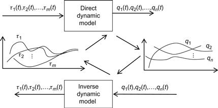
In the inverse dynamic model the inputs are the desired trajectories of the link variables, and outputs the motor torques.
3.2.1 Newton–Euler Dynamic Model
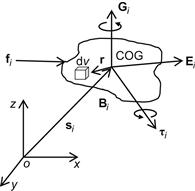
This model is derived by direct application of the Newton–Euler equations for translational and rotational motion. Consider the object ![]() (robotic link, WMR, etc.) of Figure 3.2 to which a total force
(robotic link, WMR, etc.) of Figure 3.2 to which a total force ![]() is applied at its center of gravity (COG).
is applied at its center of gravity (COG).
Then, its translational motion is described by:
![]() (3.1)
(3.1)
Here, ![]() is the linear momentum given by:
is the linear momentum given by:
![]() (3.2)
(3.2)
where ![]() is the mass of the body and
is the mass of the body and ![]() is the position of the COG with respect to the world (inertial) coordinate frame Oxyz. Assuming that
is the position of the COG with respect to the world (inertial) coordinate frame Oxyz. Assuming that ![]() is constant, then Eqs. (3.1) and (3.2) give:
is constant, then Eqs. (3.1) and (3.2) give:
![]() (3.3)
(3.3)
which is the general translational dynamic model.
The rotational motion of ![]() is described by:
is described by:
![]() (3.4)
(3.4)
where ![]() is the total angular momentum of
is the total angular momentum of ![]() with respect to COG, and
with respect to COG, and ![]() is the total external torque that produces the rotational motion of the body. The total momentum
is the total external torque that produces the rotational motion of the body. The total momentum ![]() is given by:
is given by:
![]() (3.5)
(3.5)
Here, ![]() is the inertia tensor given by the volume integral:
is the inertia tensor given by the volume integral:
![]() (3.6)
(3.6)
where ![]() is the mass density of
is the mass density of ![]() , dV is the volume of an infinitesimal element of
, dV is the volume of an infinitesimal element of ![]() lying at the position
lying at the position ![]() with respect to COG,
with respect to COG, ![]() is the angular velocity vector about the inertial axis passing from COG,
is the angular velocity vector about the inertial axis passing from COG, ![]() is the 3×3 unit matrix, and
is the 3×3 unit matrix, and ![]() is the volume of
is the volume of ![]() .
.
3.2.2 Lagrange Dynamic Model
The general Lagrange dynamic model of a solid body (multilink robot, WMR, etc.) is described by1:
![]() (3.7)
(3.7)
where ![]() is the ith-degree of freedom variable,
is the ith-degree of freedom variable, ![]() is the external generalized force vector applied to the body (i.e., force for translational motion, and torque for rotational motion), and L is the Lagrangian function defined by:
is the external generalized force vector applied to the body (i.e., force for translational motion, and torque for rotational motion), and L is the Lagrangian function defined by:
![]() (3.8)
(3.8)
Here, K is the total kinetic energy, and P the total potential energy of the body given by:
![]() (3.9)
(3.9)
where ![]() is the kinetic energy of link (degree of freedom)
is the kinetic energy of link (degree of freedom) ![]() , and
, and ![]() its potential energy. The kinetic energy K of the body is equal to:
its potential energy. The kinetic energy K of the body is equal to:
![]() (3.10)
(3.10)
where ![]() is the linear velocity of the COG,
is the linear velocity of the COG, ![]() is the angular velocity of the rotation, m is the mass, and
is the angular velocity of the rotation, m is the mass, and ![]() the inertia tensor of the body.
the inertia tensor of the body.
3.2.3 Lagrange Model of a Multilink Robot
Given a general multilink robot, the application of Eq. (3.7) leads (always) to a dynamic model of the form:
![]() (3.11a)
(3.11a)
where, for any ![]() is an
is an ![]() positive define matrix, and:
positive define matrix, and:
![]() (3.11b)
(3.11b)
is the vector of generalized variables (linear, angular) ![]() represents the inertia force,
represents the inertia force, ![]() represents the centrifugal and Coriolis force, and
represents the centrifugal and Coriolis force, and ![]() stands for the gravitational force. Since
stands for the gravitational force. Since ![]() is the net force/torque applied to the robot, if there is also friction force/torque
is the net force/torque applied to the robot, if there is also friction force/torque ![]() , then
, then ![]() where
where ![]() is the force/torque exerted by the actuators at the joints.
is the force/torque exerted by the actuators at the joints.
It is useful to note that given the model (3.11a,b) one can express the kinetic energy of the robot as:
![]() (3.12)
(3.12)
The expressions of ![]() , and
, and ![]() have to be derived in each particular case. General derivations of Eq. (3.11a) from Eq. (3.7) are given in standard industrial (fixed) robotics books.
have to be derived in each particular case. General derivations of Eq. (3.11a) from Eq. (3.7) are given in standard industrial (fixed) robotics books.
Typically, the function ![]() can be written in the form:
can be written in the form:
![]() (3.13)
(3.13)
A useful universal property of the Lagrange model given by Eqs. (3.11a)–(3.13) is that the ![]() matrix
matrix ![]() is antisymmetric, that is,
is antisymmetric, that is, ![]() .
.
3.2.4 Dynamic Modeling of Nonholonomic Robots
The Lagrange dynamic model of a nonholonomic robot (fixed or mobile) has the form (3.7):
![]() (3.14)
(3.14)
where ![]() is the
is the ![]() matrix of the
matrix of the ![]() nonholonomic constraints:
nonholonomic constraints:
![]() (3.15)
(3.15)
and ![]() is the vector Lagrange multiplier. This model leads to:
is the vector Lagrange multiplier. This model leads to:
![]() (3.16)
(3.16)
where ![]() is a nonsingular transformation matrix. To eliminate the constraint term
is a nonsingular transformation matrix. To eliminate the constraint term ![]() in Eq. (3.16) and get a constraint-free model we use an
in Eq. (3.16) and get a constraint-free model we use an ![]() matrix
matrix ![]() which is defined such that:
which is defined such that:
![]() (3.17)
(3.17)
From Eqs. (3.15) and (3.17), one can verify that there exists an ![]() -dimensional vector
-dimensional vector ![]() such that:
such that:
![]() (3.18)
(3.18)
Now, premultiplying Eq. (3.16) by ![]() and using Eqs. (3.15), (3.17), and (3.18) we get:
and using Eqs. (3.15), (3.17), and (3.18) we get:
![]() (3.19a)
(3.19a)
where:
 (3.19b)
The reduced (unconstrained) model (3.19a,b) describes the dynamic evolution of the n-dimensional vector ![]() in terms of the dynamic evolution of the
in terms of the dynamic evolution of the ![]() -dimensional vector
-dimensional vector ![]() .
.
3.3 Differential-Drive WMR
The dynamic model of the differential-drive WMR will be derived here by both the Newton–Euler and Lagrange methods.
3.3.1 Newton–Euler Dynamic Model
In the present case use will be made of the Newton–Euler equations:
![]() (3.20a)
(3.20a)
![]() (3.20b)
(3.20b)
where ![]() is the total force applied at the COG G,
is the total force applied at the COG G, ![]() is the total torque with respect to the COG m is the mass of the WMR, and I is the inertia of the WMR. Referring to Figure 2.7, and assuming that the COG G coincides with the midpoint Q (i.e., b=0), we find:
is the total torque with respect to the COG m is the mass of the WMR, and I is the inertia of the WMR. Referring to Figure 2.7, and assuming that the COG G coincides with the midpoint Q (i.e., b=0), we find:
![]() (3.21a)
(3.21a)
i.e:
![]() (3.21b)
(3.21b)
where ![]() and
and ![]() are the forces that produce the torques
are the forces that produce the torques ![]() and
and ![]() , respectively.
, respectively.
Also:
![]() (3.22)
(3.22)
Therefore, (3.20a,b) give the WMR’s dynamic model:
![]() (3.23a)
(3.23a)
![]() (3.23b)
(3.23b)
3.3.2 Lagrange Dynamic Model
We refer to Figure 2.7 and assume again that the point Q is at the position of point G. Here, the nonholonomic constraint matrix is (Eq. (2.42)):
![]() (3.24)
(3.24)
Since the WMR moves on a horizontal planar terrain, the terms ![]() and
and ![]() in Eq. (3.16) are zero. Therefore, the model (3.16) becomes:
in Eq. (3.16) are zero. Therefore, the model (3.16) becomes:
![]() (3.25)
(3.25)
where:
 (3.26a)
 (3.26b)
To convert the model (3.25) to the corresponding unconstrained model (3.19a,b), we need the matrix ![]() in (3.17). Here, this matrix is:
in (3.17). Here, this matrix is:
 (3.27)
which satisfies Eq. (3.17). Therefore, Eq. (3.19b) gives:
![]() (3.28)
(3.28)
and the model (3.19a) becomes:
![]() (3.29)
(3.29)
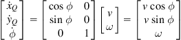
Noting that ![]() is the translation velocity v and
is the translation velocity v and ![]() the angular velocity
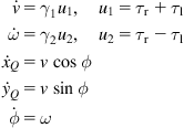
the angular velocity ![]() of the robot, Eq. (3.29) gives the model:
of the robot, Eq. (3.29) gives the model:
![]() (3.30a)
(3.30a)
![]() (3.30b)
(3.30b)
which is identical to Eq. (3.23a,b), as expected. Finally, using Eq. (3.18) we get:
 (3.31)
which is the WMR’s kinematic model. The dynamic and kinematic Eqs. (3.30a,b) and (3.31) describe fully the motion of the differential-drive WMR.
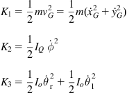
Example 3.1
The problem is to derive the Lagrange dynamic model using directly the Lagrangian function L for a differential-drive WMR in which:
1. There is linear friction in the wheels with the same friction coefficient.
Solution
We will work with the WMR of Figure 2.7.The kinetic energy K of the robot is given by:
![]() (3.32)
(3.32)
where:
 (3.33)
and (Example 2.2):
![]()
![]() =moment of inertia of the robot with respect to Q
=moment of inertia of the robot with respect to Q
![]() =moment of inertia of each wheel plus the corresponding motor’s rotor moment of inertia.
=moment of inertia of each wheel plus the corresponding motor’s rotor moment of inertia.
The velocities ![]() , and
, and ![]() are given by Eq. (2.36a–c):
are given by Eq. (2.36a–c):
 (3.34)
Using Eqs. (3.33) and (3.34) in Eq. (3.32) the total kinetic energy K of the robot is found to be:
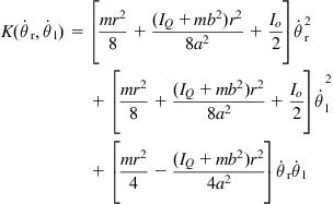 (3.35)
Here the kinetic energy is expressed directly in terms of the angular velocities ![]() and
and ![]() of the driving wheels. The Lagrangian L is equal to K, since the robot is moving on a horizontal plane and so the potential energy P is zero. Therefore, the Lagrange dynamic equations of this robot are:
of the driving wheels. The Lagrangian L is equal to K, since the robot is moving on a horizontal plane and so the potential energy P is zero. Therefore, the Lagrange dynamic equations of this robot are:
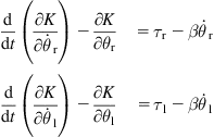 (3.36)
where β is the wheels’ common friction coefficient, and ![]() are the right and left actuation torques. Using (3.35) in (3.36) we get:
are the right and left actuation torques. Using (3.35) in (3.36) we get:
![]() (3.37)
(3.37)
where:
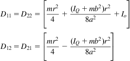 (3.38)
3.3.3 Dynamics of WMR with Slip
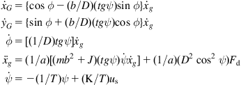
Here we will derive the Newton–Euler dynamic model of the slipping differential-drive WMR considered in Example 2.2. The case where both longitudinal slip (variables ![]() ) and lateral slip (variables
) and lateral slip (variables ![]() ) are present will be considered [5].
) are present will be considered [5].
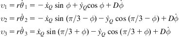
For convenience we write again the kinematic equations of the robot (with steering angles ![]() ):
):
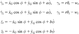
Defining the generalized variables’ vector ![]() as:
as:
![]() (3.39)
(3.39)
the above relations can be written in the following Pfaffian matrix form:
![]()
where:
 (3.40)
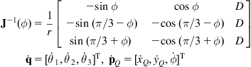
The matrix ![]() and the velocity vector
and the velocity vector ![]() that satisfy the relations (Eqs. (3.17)–(3.18)):
that satisfy the relations (Eqs. (3.17)–(3.18)):
![]() (3.41)
(3.41)
 (3.42)
where:
![]() (3.43a)
(3.43a)
 (3.43b)
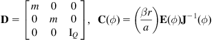
To derive the Newton–Euler dynamic model we draw the free-body diagram of the WMR body without the wheels (Figure 3.3), and the free-body diagram of the two wheels (Figure 3.4).
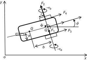

Figure 3.4 Force–torque diagram of the two wheels. The coordinate frame ![]() is fixed at the driving wheels’ midpoint.
is fixed at the driving wheels’ midpoint.
In Figures 3.3 and 3.4, we have the following dynamic parameters and variables:
![]() : The torque given to the wheels by the body of the WMR
: The torque given to the wheels by the body of the WMR
![]() : The driving torques exerted to the right and left wheel by their motors
: The driving torques exerted to the right and left wheel by their motors
![]() : The mass of the WMR body without the wheels
: The mass of the WMR body without the wheels
![]() : The mass of each driving wheel assembly (wheel plus DC motor of the robot body)
: The mass of each driving wheel assembly (wheel plus DC motor of the robot body)
![]() : The moment of inertia about a vertical axis passing via G (without the wheels)
: The moment of inertia about a vertical axis passing via G (without the wheels)
![]() : The wheel moment of inertia about its axis
: The wheel moment of inertia about its axis
![]() : The wheel moment of inertia about its diameter
: The wheel moment of inertia about its diameter
![]() : The reaction forces between the WMR body and the wheels
: The reaction forces between the WMR body and the wheels
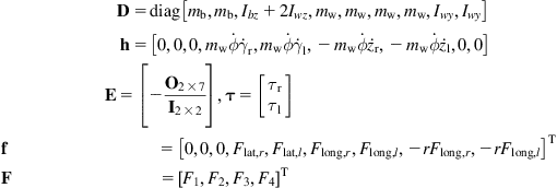
Using the above notation, the Newton–Euler dynamic equations of the robot, written down for each generalized variable in the vector (3.39), are:
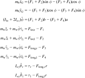 (3.44)
where ![]() .
.
The detailed Eq. (3.44) can be written in the compact form of Eq. (3.16), namely:
![]() (3.45)
(3.45)
where ![]() is given by (3.40), and:
is given by (3.40), and:
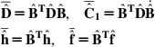
Applying to Eq. (3.45) the procedure of Section 3.2.4, we get the following reduced model (3.19a,b):
![]() (3.46)
(3.46)
where:
![]()
The model (3.46) can be split as:
![]() (3.47a)
(3.47a)
![]() (3.47b)
(3.47b)
![]() (3.47c)
(3.47c)
where:
![]()
![]()
![]()
![]()
![]()
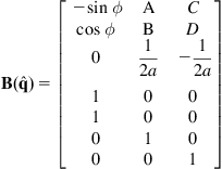 (3.48)
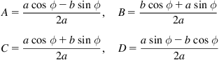
with A, B, C, and D as in Eq. (3.43b). Writing ![]() in the form of Eq. (3.13), that is,
in the form of Eq. (3.13), that is, ![]() , the model (3.47a) takes the form:
, the model (3.47a) takes the form:
![]() (3.49)
(3.49)
where:
![]()
Finally, Eq. (3.47b,c) can be written in the matrix form:
![]() (3.50)
(3.50)
where:
![]() (3.51)
(3.51)
To summarize, the dynamic model of the differential-drive WMR with slip is:
![]() (3.52a)
(3.52a)
![]() (3.52b)
(3.52b)
with:
![]() (3.52c)
(3.52c)
3.4 Car-Like WMR Dynamic Model
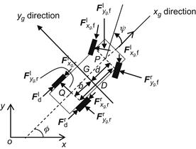
The kinematic equations of the car-like WMR were derived in Section 2.6. Here, we will derive the Newton–Euler dynamic model for a four-wheel rear-drive front-steer WMR [9]. The equivalent bicycle model shown in Figure 3.5 will be used.

The WMR is subject to the driving force ![]() and two lateral slip forces
and two lateral slip forces ![]() and
and ![]() applied perpendicular to the corresponding wheels. Before presenting the dynamic equations we derive the nonholonomic constraints that apply to the COG G which lies at a distance b from Q, and a distance d from P. To this end, we start with the nonholonomic constraints (2.50a,b) that refer to the points Q and P:
applied perpendicular to the corresponding wheels. Before presenting the dynamic equations we derive the nonholonomic constraints that apply to the COG G which lies at a distance b from Q, and a distance d from P. To this end, we start with the nonholonomic constraints (2.50a,b) that refer to the points Q and P:
![]() (3.53)
(3.53)
Denoting by ![]() and
and ![]() the coordinates of the point G in the world coordinate frame we get:
the coordinates of the point G in the world coordinate frame we get:
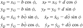 (3.54)
Introducing the relations (3.54) into (3.53) yields:
![]() (3.55)
(3.55)
Now, denoting by ![]() the velocity of the COG G in the local coordinate frame
the velocity of the COG G in the local coordinate frame ![]() and applying the rotational transformation (2.17) (Example 2.1) we get:
and applying the rotational transformation (2.17) (Example 2.1) we get:
![]() (3.56)
(3.56)
Introducing Eq. (3.56) into Eq. (3.55) yields:
![]() (3.57)
(3.57)
which, upon differentiation, give:
![]() (3.58a)
(3.58a)
![]() (3.58b)
(3.58b)
From Eqs. (3.57) and (3.58a,b) we get:
![]() (3.59)
(3.59)
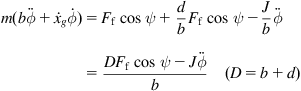
Referring to Figure 3.5 we obtain the following Newton–Euler dynamic equations:
![]() (3.60a)
(3.60a)
![]() (3.60b)
(3.60b)
![]() (3.60c)
(3.60c)
![]() (3.60d)
(3.60d)
![]() =moment of inertia of the WMR about G
=moment of inertia of the WMR about G
![]() =front and rear wheel lateral forces
=front and rear wheel lateral forces
![]() =time constant of the steering system
=time constant of the steering system
![]() =a constant coefficient (gain)
=a constant coefficient (gain)
![]() , with r the rear wheel radius, and
, with r the rear wheel radius, and ![]() the applied motor torque.2
the applied motor torque.2
We will now put the above dynamic equations into state space form, where the state vector is:
![]() (3.61)
(3.61)
To this end, we solve Eq. (3.60c) for ![]() and introduce it, together with Eq. (3.58a) into (3.60b) to get:
and introduce it, together with Eq. (3.58a) into (3.60b) to get:
![]() (3.62)
(3.62)
Now introducing Eqs. (3.57), (3.58b), and (3.62) into Eq. (3.60a) we get:
![]() (3.63a)
(3.63a)
where:
![]() (3.63b)
(3.63b)
Finally, introducing Eq. (3.57) into Eq. (3.56) gives:
 (3.64)
with ![]() . The model (3.64) represents an affine system with two inputs
. The model (3.64) represents an affine system with two inputs ![]() , a five-dimensional state vector:
, a five-dimensional state vector:
![]() (3.65a)
(3.65a)
a drift term:
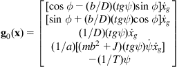 (3.65b)
and the two input fields:
![]() (3.65c)
(3.65c)
namely:
![]() (3.66)
(3.66)
3.5 Three-Wheel Omnidirectional Mobile Robot
Here, we will derive the dynamic model of a three-wheel omnidirectional robot using the Newton–Euler method [10]. This derivation is the same for any number of universal (orthogonal) omniwheels. Some further studies of omnidirectional WMRs are presented in Refs. [11–14].
Consider the WMR in the pose shown in Figure 3.6 in which the three wheels are placed at angles ![]() , respectively.
, respectively.

The rotation matrix of the robot’s local coordinate frame ![]() with respect to the world coordinate frame
with respect to the world coordinate frame ![]() is:
is:
![]() (3.67)
(3.67)
Let ![]() be the position vector of the COG
be the position vector of the COG ![]() . Then:
. Then:
![]() (3.68)
(3.68)
where ![]() , m is the robot’s mass, and
, m is the robot’s mass, and ![]() is the force exerted at the COG expressed in the world coordinate frame. Denoting by:
is the force exerted at the COG expressed in the world coordinate frame. Denoting by:
![]() (3.69)
(3.69)
the position vector of the COG and the force vector expressed in the local (moving) coordinate frame, then Eq. (3.67) implies that:
![]() (3.70)
(3.70)
Thus, using Eq. (3.70) in Eq. (3.68) we get:
![]() (3.71)
(3.71)
Now, the dynamic equation of the rotation about the COG Q is:
![]() (3.72)
(3.72)
where ![]() is the moment of inertia of the robot about Q, and
is the moment of inertia of the robot about Q, and ![]() is the applied torque at Q.
is the applied torque at Q.
From the geometry of Figure 3.6 we obtain:
 (3.73)
where D is the distance of the wheels from the rotation point Q, and ![]() are the driving forces of the wheels.
are the driving forces of the wheels.
The rotation of each wheel is described by the dynamic equation:
![]() (3.74)
(3.74)
where ![]() is the common moment of inertia of the wheels,
is the common moment of inertia of the wheels, ![]() is the angular position of wheel
is the angular position of wheel ![]() ,
, ![]() is the linear friction coefficient,
is the linear friction coefficient, ![]() is the common radius of the wheels,
is the common radius of the wheels, ![]() is the driving input torque of wheel
is the driving input torque of wheel ![]() , and
, and ![]() is the driving torque gain.
is the driving torque gain.
Now, from the geometry of Figure 3.6 we see that the angles of the wheel velocities in the local coordinate frame are: ![]()
Thus, we obtain the inverse kinematics equations from ![]() to
to ![]() as:
as:
![]() (3.75a)
(3.75a)
![]() (3.75b)
(3.75b)
![]() (3.75c)
(3.75c)
Using Eqs. (3.69)–(3.75c) we get after some algebraic manipulation:
![]() (3.76a)
(3.76a)
![]() (3.76b)
(3.76b)
![]() (3.76c)
(3.76c)
![]()
![]()
Finally, combining Eqs. (3.67), (3.68), and (3.76a–c) we get the following state–space dynamic model of the WMR’s motion:
![]() (3.77a)
(3.77a)
![]() (3.77b)
(3.77b)
where:


The azimuth of the robot in the world coordinate frame is denoted by ![]() , where
, where ![]() (
(![]() denotes the angle between
denotes the angle between ![]() and
and ![]() , that is, the azimuth of the robot in the moving coordinate frame). Then:
, that is, the azimuth of the robot in the moving coordinate frame). Then:
![]()
Whence:
![]() (3.78)
(3.78)
where the positive direction is the counterclockwise rotation direction. It is noted that the motions along ![]() and
and ![]() are coupled because the dynamic equations are derived in the world coordinate frame. But since the rotational angle is always equal to
are coupled because the dynamic equations are derived in the world coordinate frame. But since the rotational angle is always equal to ![]() , despite the fact that
, despite the fact that ![]() may be changing arbitrarily, the WMR can realize a translational motion without changing the pose (i.e., the WMR is holonomic). The model (3.77a) can be written in a three-input affine form with drift as follows:
may be changing arbitrarily, the WMR can realize a translational motion without changing the pose (i.e., the WMR is holonomic). The model (3.77a) can be written in a three-input affine form with drift as follows:
![]() (3.79)
(3.79)
where:
![]()
The dynamic model (3.77a) of a three-wheel omnidirectional robot (with universal wheels) is one of the many different models available. Actually, many other equivalent models were derived in the literature.
Example 3.2
Derive the dynamic equations of the three-wheel omnidirectional robot using the unit directional vectors ![]() of the wheel velocities.
of the wheel velocities.
Solution
To simplify the derivation we select the pose of the WMR in which the wheel 1 orientation is perpendicular to the local coordinate axis ![]() as shown in Figure 3.7 [15]. Thus the unit directional vectors
as shown in Figure 3.7 [15]. Thus the unit directional vectors ![]() , and
, and ![]() are:
are:
![]() (3.80)
(3.80)

The rotational matrix of ![]() with respect to
with respect to ![]() is given by (3.67).
is given by (3.67).
Therefore, the driving velocities ![]() of the wheels are:
of the wheels are:
or
![]() (3.81)
(3.81)
where:
This is the inverse kinematic model of the robot. Now, applying the Newton–Euler method to the robot we get:
![]() (3.82a)
(3.82a)
![]() (3.82b)
(3.82b)
where ![]() is the magnitude of the driving force of the ith wheel, m is the robot mass,
is the magnitude of the driving force of the ith wheel, m is the robot mass, ![]() is the robot moment of inertia about Q, and:
is the robot moment of inertia about Q, and:
![]() (3.83)
(3.83)
are two-dimensional vectors found using Eqs. (3.67) and (3.80). The driving forces ![]()
![]() are given by the relation:
are given by the relation:
![]() (3.84)
(3.84)
where ![]() is the voltage applied to the motor of the ith wheel, “a” is the voltage–force constant, and
is the voltage applied to the motor of the ith wheel, “a” is the voltage–force constant, and ![]() is the friction coefficient.
is the friction coefficient.
Combining Eqs. (3.82a,b), (3.83), and (3.84) we obtain the model:
![]() (3.85a)
(3.85a)
where:
 (3.85b)
 (3.85c)
The model (3.85a–c) has the standard form of the robot model described by Eqs. (3.11) and (3.13).
Example 3.3
We are given a car-like robot where there are lateral slip forces and longitudinal friction forces on all wheels. It is desired to write down the Newton–Euler dynamic equations in the form (3.60a–d).
Solution
The free-body diagram of the robot is as shown in Figure 3.8.
We use the following definitions:
where the upper index r refers to the right wheel and the upper index l to the left wheel. Therefore, considering the bicycle model of the WMR we get the following Newton–Euler dynamic equations in the local coordinate frame:

where all variables have the meaning presented in Section 3.4. From this point the development of the full model can be done as in Section 3.4.
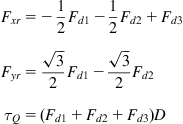
3.6 Four Mecanum-Wheel Omnidirectional Robot
We consider the four-wheel omnidirectional robot of Figure 3.9A [3].
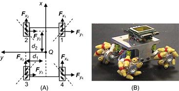
Figure 3.9 (A) The four-wheel mecanum WMR and the forces acting on it and (B) an experimental four-wheel mecanum WMR prototype. Source: www.robotics.ee.uwa.edu.au/eyebot/doc/robots/omni.html.
The total forces ![]() and
and ![]() acting on the robot in the x and y directions are:
acting on the robot in the x and y directions are:
![]() (3.86a)
(3.86a)
![]() (3.86b)
(3.86b)
where ![]() are the forces acting on the wheels along the x and y axes. In the absence of separate rotation motion, the direction of motion is defined by an angle
are the forces acting on the wheels along the x and y axes. In the absence of separate rotation motion, the direction of motion is defined by an angle ![]() where:
where:
![]() (3.87)
(3.87)
The torque ![]() that produces pure rotation is:
that produces pure rotation is:
![]() (3.88)
(3.88)
where positive rotation is in the counterclockwise direction.
The Newton–Euler motion equations are:
![]() (3.89a)
(3.89a)
![]() (3.89b)
(3.89b)
![]() (3.89c)
(3.89c)
where ![]() , and
, and ![]() are the linear friction coefficients in the x, y, and
are the linear friction coefficients in the x, y, and ![]() motion, and
motion, and ![]() are the mass and moment of inertia of the robot. Equations (3.89a–c) show that the robot can achieve steady-state velocities
are the mass and moment of inertia of the robot. Equations (3.89a–c) show that the robot can achieve steady-state velocities ![]() and
and ![]() equal to:
equal to:
![]() (3.90)
(3.90)
Example 3.4
The problem is to calculate the wheel angular velocities which are required to achieve a desired translational and rotational motion (WMR velocities v and ![]() ) of the mecanum mobile robot of Figure 3.9A.
) of the mecanum mobile robot of Figure 3.9A.
Solution
A solution to this problem was provided by the relations (2.84) and (2.85). Here we will provide an alternative method [3]. We draw the displacement and velocity vectors of a single wheel which are as shown in Figure 3.10A and B, where “![]() ” is the roller angle
” is the roller angle ![]() .
.
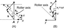
Figure 3.10 (A) Displacement vectors of a wheel and roller and (B) velocity vectors (![]() is the rollers angle).
is the rollers angle).
The vector ![]() represents the displacement due to the wheel rotation (in the positive direction),
represents the displacement due to the wheel rotation (in the positive direction), ![]() represents the displacement vector due to rolling which is orthogonal to the roller axis, and
represents the displacement vector due to rolling which is orthogonal to the roller axis, and ![]() represents the total displacement vector. The dotted horizontal lines represent the discontinuities where the roller contact point transfers from one roller to the next. In Figure 3.10, the point A was selected in the middle of this discontinuity line to facilitate the calculation.
represents the total displacement vector. The dotted horizontal lines represent the discontinuities where the roller contact point transfers from one roller to the next. In Figure 3.10, the point A was selected in the middle of this discontinuity line to facilitate the calculation.
From Figure 3.10B we get ![]() because the components of
because the components of ![]() and
and ![]() along the roller axis are equal. Therefore:
along the roller axis are equal. Therefore:
![]() (3.91)
(3.91)
for ![]() . If
. If ![]() , the rotation of the wheel does not produce translation motion of the rollers. Solving Eq. (3.91) for v we get:
, the rotation of the wheel does not produce translation motion of the rollers. Solving Eq. (3.91) for v we get:
![]() (3.92)
(3.92)
When ![]() , the rotational speed
, the rotational speed ![]() of the wheel must be zero, but the wheel can have any value of translation velocity because of the motion of the other wheels.
of the wheel must be zero, but the wheel can have any value of translation velocity because of the motion of the other wheels.
We now calculate the wheel angular velocity ![]() for a desired translational motion velocity v. From Eq. (3.90), we see that the wheel velocity is proportional to the forces applied by each wheel, that is:
for a desired translational motion velocity v. From Eq. (3.90), we see that the wheel velocity is proportional to the forces applied by each wheel, that is:
“![]() proportional to
proportional to ![]() ,” and because the WMR is a rigid body, all wheels should have the same translational speed, that is:
,” and because the WMR is a rigid body, all wheels should have the same translational speed, that is:
![]()
Therefore, from Eq. (3.92) we have:
![]() (3.93)
(3.93)
Equation (3.93) gives the velocities ![]() of the four wheels needed to get a desired translational velocity v of the robot.
of the four wheels needed to get a desired translational velocity v of the robot.
Finally, we will calculate the wheel angular velocities required to get a desired rotational speed ![]() . Consider a robot with velocity v. Then the instantaneous curvature radius (ICR) of its path is:
. Consider a robot with velocity v. Then the instantaneous curvature radius (ICR) of its path is:
![]() (3.94)
(3.94)
These relations give the following world frame coordinates ![]() of the ICR (Figure 3.11):
of the ICR (Figure 3.11):
![]()

Figure 3.11 Geometry of wheel i with reference to the coordinate frame ![]() . Each wheel has its own total velocity
. Each wheel has its own total velocity ![]() and angle
and angle ![]() .
.
The geometry of each wheel is defined by its position ![]() and the orientation
and the orientation ![]() of its rollers. Let
of its rollers. Let ![]() be the contact point of wheel i then:
be the contact point of wheel i then:
![]() (3.95)
(3.95)
where ![]() is the same for all wheels due to the symmetry of the wheels with respect to the point Q. The distance
is the same for all wheels due to the symmetry of the wheels with respect to the point Q. The distance ![]() of the ICR and the contact point
of the ICR and the contact point ![]() is given by the triangle formula, as:
is given by the triangle formula, as:
![]() (3.96)
(3.96)
The velocity ![]() of the wheel should be perpendicular to the line
of the wheel should be perpendicular to the line ![]() . Therefore, the angle
. Therefore, the angle ![]() of the line
of the line ![]() with the x-axis is determined by the relation:
with the x-axis is determined by the relation:
![]() (3.97)
(3.97)
whence:
![]() (3.98)
(3.98)
because, in Figure 3.11, ![]() is actually negative
is actually negative ![]() . Now, in view of Eq. (3.94) we have:
. Now, in view of Eq. (3.94) we have:
![]() (3.99)
(3.99)
Finally, using Eq. (3.99), Eq. (3.93) gives:
![]() (3.100)
(3.100)
for ![]() , where r is the common radius of the wheels. Equation (3.100) gives the required rotational speeds of the wheels in terms of the position
, where r is the common radius of the wheels. Equation (3.100) gives the required rotational speeds of the wheels in terms of the position ![]() of ICR and the desired rotational speed
of ICR and the desired rotational speed ![]() of the robot. Actually, in view of Eqs. (3.94) and (3.96), Eq. (3.100) gives
of the robot. Actually, in view of Eqs. (3.94) and (3.96), Eq. (3.100) gives ![]() in terms of the known (desired) values of
in terms of the known (desired) values of ![]() ,
, ![]() ,
, ![]() , and
, and ![]() .
.
Example 3.5
It is desired to describe a way for identifying the dynamic parameters of a differential-drive WMR by converting its dynamic model to a linear form which uses the robot linear displacement in place of ![]() , and
, and ![]() .
.
The nonlinear dynamic model of this WMR is given by Eqs. (3.30a,b) and (3.31) which is written as:
where ![]() and
and ![]() are the dynamic parameters to be identified. Using the robot’s linear displacement:
are the dynamic parameters to be identified. Using the robot’s linear displacement:
![]()
in place of the components ![]() and
and ![]() (Figure 2.7) we get the linear model:
(Figure 2.7) we get the linear model:
![]()
which reduces to:
![]() (3.101)
(3.101)
This is a linear model with two outputs ![]() and
and ![]() . The identification will be made rendering the model (3.101) to the standard linear regression model:
. The identification will be made rendering the model (3.101) to the standard linear regression model:
![]() (3.102)
(3.102)
where:
![]()
The matrix ![]() is known as “regressor matrix.” Under the assumption that
is known as “regressor matrix.” Under the assumption that ![]() is independent of
is independent of ![]() , and
, and ![]() the solution for
the solution for ![]() is given by3:
is given by3:
![]() (3.103)
(3.103)
To convert Eq. (3.101) into the regression form (3.102) we discretize it in time using the first order approximation: ![]() , where
, where ![]() and
and ![]() is the sampling period. Then, Eq. (3.101) becomes:
is the sampling period. Then, Eq. (3.101) becomes:
![]() (3.104)
(3.104)
where ![]() . Clearly, the parameters
. Clearly, the parameters ![]() and
and ![]() are identifiable, but the difficulty is that
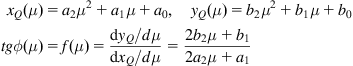
are identifiable, but the difficulty is that ![]() cannot be measured. To overcome this difficulty we use a second-order parametric representation of
cannot be measured. To overcome this difficulty we use a second-order parametric representation of ![]() , and
, and ![]() , namely [16]:
, namely [16]:
with boundary conditions:
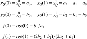
From the above conditions, the parameters ![]() and
and ![]()
![]() are computed as:
are computed as:
![]() (3.105a)
(3.105a)
![]() (3.105b)
(3.105b)
The approximate length increment ![]() of
of ![]() is given by:
is given by:
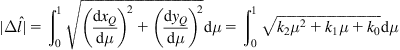 (3.106a)
where:
![]() (3.106b)
(3.106b)
Equation (3.106a) is an integral equation, the close solution of which is available in integral tables. The sign of ![]() , which determines whether the robot moved forward or backward, can be determined by the following relation:
, which determines whether the robot moved forward or backward, can be determined by the following relation:
![]()
where ![]() is the current position and
is the current position and ![]() is the past position of the robot. Several numerical experiments performed using the above WMR identification method gave very satisfactory results for both
is the past position of the robot. Several numerical experiments performed using the above WMR identification method gave very satisfactory results for both ![]() and
and ![]() [16].
[16].
3Equation (3.103) can be found by minimizing the function ![]() with respect to
with respect to ![]() . An easy way to get Eq. (3.103) is by multiplying Eq. (3.102) by
. An easy way to get Eq. (3.103) is by multiplying Eq. (3.102) by ![]() and solving for
and solving for ![]() , under the assumption that
, under the assumption that ![]() (
(![]() independent of
independent of ![]() ,and rank
,and rank ![]() . Actually, Eq. (3.103) is
. Actually, Eq. (3.103) is ![]() where
where ![]() is the generalized inverse of
is the generalized inverse of ![]() (Eq. (2.8a)).
(Eq. (2.8a)).
Example 3.6
Outline a method for applying the least squares identification model (3.102)–(3.103) to the general nonholonomic WMR model (3.19a–b)
Solution
![]()
is put in the form:
![]()
where ![]() is the vector of unknown parameters The above model can be written in the form (3.102) by computing
is the vector of unknown parameters The above model can be written in the form (3.102) by computing ![]() as:
as:
 (3.107)
where ![]() and T is the sampling period of the measurements.
and T is the sampling period of the measurements.
Now, defining ![]() and
and ![]() as:
as:

The model (3.107), after N measurements, becomes:
![]() (3.108)
(3.108)
This method overcomes the noise problem posed by the calculation of the acceleration. The optimal estimate ![]() of
of ![]() is given by Eq. (3.103):
is given by Eq. (3.103):
![]() (3.109)
(3.109)
The identification process can be simplified if it is split in two parts, namely: (i) identification when the robot is moving on a line without rotation, and (ii) identification when the robot has pure rotation movement. In the pure linear motion we keep the angle ![]() constant (i.e.,
constant (i.e., ![]() ), and in the pure rotation motion we have
), and in the pure rotation motion we have ![]() (i.e.,
(i.e., ![]() and
and ![]() ) [17].
) [17].
References
1. McKerrow PK. Introduction to robotics Reading, MA: Addison-Wesley; 1999.
2. Dudek G, Jenkin M. Computational principles of mobile robotics Cambridge: Cambridge University Press; 2010.
3. De Villiers M, Bright G. Development of a control model for a four-wheel mecanum vehicle. In: Proceedings of twenty fifth international conference of CAD/CAM robotics and factories of the future conference. Pretoria, South Africa; July 2010.
4. Song JB, Byun KS. Design and control of a four-wheeled omnidirectional mobile robot with steerable omnidirectional wheels. J Rob Syst. 2004;21:193–208.
5. Sidek SN. Dynamic modeling and control of nonholonomic wheeled mobile robot subjected to wheel slip. PhD Thesis, Vanderbilt University, Nashville, TN, December 2008.
6. Williams II RL, Carter BE, Gallina P, Rosati G. Dynamic model with slip for wheeled omni-directional robots. IEEE Trans Rob Autom. 2002;18(3):285–293.
7. Stonier D, Se-Hyoung C, Sung–Lok C, Kuppuswamy NS, Jong-Hwan K. Nonlinear slip dynamics for an omniwheel mobile robot platform. In: Proceedings of IEEE international conference on robotics and automation. Rome, Italy; April 10–14, 2007. p. 2367–72.
8. Ivanjko E, Petrinic T, Petrovic I. Modeling of mobile robot dynamics. In: Proceedings of seventh EUROSIM congress on modeling and simulation. Prague, Czech Republic; September 6–9, 2010. p. 479–86.
9. Moret EN. Dynamic modeling and control of a car-like robot. MSc Thesis, Virginia Polytechnic Institute and State University, Blacksburg, VA, February 2003.
10. Watanabe K, Shiraishi Y, Tzafestas SG, Tang J, Fukuda T. Feedback control of an omnidirectional autonomous platform for mobile service robots. J Intell Rob Syst. 1998;22:315–330.
11. Pin FG, Killough SM. A new family of omnidirectional and holonomic wheeled platforms for mobile robots. IEEE Trans Rob Autom. 1994;10(4):480–489.
12. Rojas R. Omnidirectional control. Freie University, Berlin; May 2005. <http://robocup.mi.fu-berlin.de/buch/omnidrive.pdf>.
13. Connette CP, Pott A, Hagele M, Verl A. Control of a pseudo-omnidirectional, non-holonomic, mobile robot based on an ICM representation in spherical coordinates. In: Proceedings of 47th IEEE conference on decision and Control. Canum, Mexico; December 9–11, 2008. p. 4976–83.
14. Moore KL, Flann NS. A six-wheeled omnidirectional autonomous mobile robot. IEEE Control Syst Mag. 2000;20(6):53–66.
15. Kalmar-Nagy T, D’Andrea R, Ganguly P. Near-optimal dynamic trajectory generation and control of an omnidirectional vehicle. Rob Auton Syst. 2007;46:47–64.
16. Cuerra PN, Alsina PJ, Medeiros AAD, Araujo A. Linear modeling and identification of a mobile robot with differential drive. In: Proceedings of ICINCO international conference on informatics in control automation and robotics. Setubal, Portugal; 2004. p. 263–9.
17. Handy A, Badreddin E. Dynamic modeling of a wheeled mobile robot for identification, navigation and control. In: Proceedings of IMACS conference on modeling and control of technological systems. Lille, France; 1992. p. 119–28.
1Derivations of Eq. (3.7) from first principles are provided in textbooks on mechanics.
2Here, the driving motor dynamics is not included. Derivation of DC motor dynamic models is provided in Example 5.1.