
Experimental Studies
The objective of this chapter is to present a collection of experimental simulation results drawn from the open literature for most of the methodologies considered in the book. Specifically, the book provides sample results obtained under various artificial and realistic conditions. In most cases, the desired paths to be followed and the trajectories to be tracked are straight lines, curved lines, or circles or appropriate combinations of them. The simulation experiments presented in the chapter cover the following problems treated in the book: (i) Lyapunov-based model reference adaptive and robust control, (ii) pose stabilization and parking control using polar, chained, and Brockett-type integrator models, (iii) deterministic and fuzzy sliding mode control, (iv) vision-based control of mobile robots and mobile manipulators, (v) fuzzy path planning in unknown environments (local, global, and integrated global-local path planning), (vi) fuzzy tracking control of differential drive WMR, and (vii) simultaneous localization and mapping (SLAM) using extended Kalman filters (EKFs) and particle filters (PFs).
Keywords
Feature error vector evolution; local model network; supervised tracking neurocontroller; controller performance; pose stabilizing control; robot cooperation; parking control; EKF errors; parking maneuvering; constrained dynamic control; reduced complexity sliding mode FLC; Takagi–Sugeno fuzzy model; coordinated open/closed-loop control; omnidirectional image; control performance; maximum manipulability control; fuzzy neural path planning
13.1 Introduction
In this book, we have presented fundamental analytic methodologies for the derivation of wheeled mobile robot (WMR) kinematic and dynamic models, and the design of several controllers. Unavoidably, these methodologies represent a small subset of the variations and extensions available in the literature, but the material included in the book is over sufficient for its introductory purposes, taking into account the required limited size of the book. All methods reported in the open literature are supported by simulation experimental results, and in many cases, the methods were applied and tested in real research mobile robots and manipulators.
The objective of this chapter is to present a collection of experimental simulation and physical results drawn from the open literature for most of the methodologies considered in the book. Specifically, the book provides sample results obtained under various artificial and realistic conditions. In most cases, the desired paths to be followed and the trajectories to be tracked are straight lines, curved lines, or circles or appropriate combinations of them. The experiments presented in the chapter cover the following problems treated in the book:
• Lyapunov-based model-based adaptive and robust control
• Pose stabilization and parking control using polar, chained, and Brockett-type integrator models
• Deterministic and fuzzy sliding mode control
• Vision-based control of mobile robots and mobile manipulators
• Fuzzy path planning in unknown environments (local, global, and integrated global–local path planning)
• Fuzzy tracking control of differential drive WMR
• Neural network-based tracking control and obstacle avoiding navigation
• Simultaneous localization and mapping (SLAM) using extended Kalman filters (EKFs) and particle filters (PFs)
By necessity, hardware, software, or numerical details are not included in the chapter. But, most of the simulation results were obtained using Matlab/Simulink functions. The reader is advised to reproduce some of the results with personal simulation or physical experiments.
13.2 Model Reference Adaptive Control
Model reference adaptive control was studied in Chapter 7. Two equivalent controllers were derived. The first of them is given by Eqs. (7.40a), (7.40b), and (7.41), and the second is given by Eq. (7.77). In both cases, the mass ![]() and the moment of inertia
and the moment of inertia ![]() of the WMR were considered to be unknown constants or slowly varying parameters. Starting the operation of the controllers using available initial guessed values of these parameters, the adaptive controllers perform simultaneously two tasks, namely, updating (adapting) the parameter values and stabilizing the tracking of the desired trajectories. As the time passes, the parameters approach their true values, and the tracking performance is improved. This fact has been verified by simulation of the controllers [1,2]. Figure 13.1A–C shows the performance of the first controller achieved with gain values
of the WMR were considered to be unknown constants or slowly varying parameters. Starting the operation of the controllers using available initial guessed values of these parameters, the adaptive controllers perform simultaneously two tasks, namely, updating (adapting) the parameter values and stabilizing the tracking of the desired trajectories. As the time passes, the parameters approach their true values, and the tracking performance is improved. This fact has been verified by simulation of the controllers [1,2]. Figure 13.1A–C shows the performance of the first controller achieved with gain values ![]() and adaptation parameters
and adaptation parameters ![]() . The true parameter values are
. The true parameter values are ![]() and
and ![]() . The mobile robot initial pose is
. The mobile robot initial pose is ![]() ,
, ![]() , and
, and ![]() . Figure 13.1A depicts the convergence of the errors
. Figure 13.1A depicts the convergence of the errors ![]() ,
, ![]() , and
, and ![]() using the true values. Figure 13.1B and C shows the error convergence performance when the initial parameter values of the nonadaptive and adaptive controller are
using the true values. Figure 13.1B and C shows the error convergence performance when the initial parameter values of the nonadaptive and adaptive controller are ![]() and
and ![]() , respectively.
, respectively.
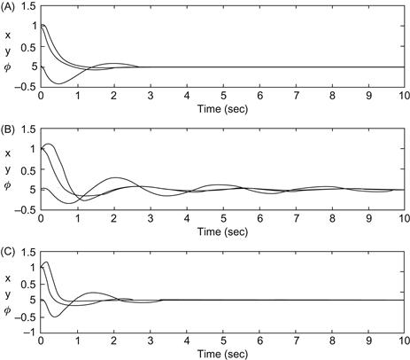
Figure 13.1 (A) Convergence with the true ![]() and
and ![]() values. (B) Convergence of the nonadaptive controller when the initial parameters are
values. (B) Convergence of the nonadaptive controller when the initial parameters are ![]() and
and ![]() . (C) Convergence of the adaptive controller with the same initial parameter values. Source: Reprinted from Ref. [1], with permission from European Union Control Association.
. (C) Convergence of the adaptive controller with the same initial parameter values. Source: Reprinted from Ref. [1], with permission from European Union Control Association.
The convergence when the true parameter values are used in the controller is achieved at 3 s (Figure 13.1A). The convergence of the nonadaptive controller when the parameter values are different from the true ones is achieved after 10 s (Figure 13.1B), and the convergence of the adaptive controller is achieved at about 4 s. The above results illustrate the robustness of the adaptive controller against parameter uncertainties. Analogous performance was obtained with the second adaptive controller [2]. The WMR parameters used in Ref. [2] are ![]() (true values of unknown dynamic parameters with known signs),
(true values of unknown dynamic parameters with known signs), ![]() , and
, and ![]() . Two cases were studied, namely, (i) a
. Two cases were studied, namely, (i) a ![]() straight-line desired trajectory
straight-line desired trajectory ![]() and (ii) a unity radius circular trajectory, centered at the origin, produced by a moving point with constant linear velocity 0.5 m/s and initial pose
and (ii) a unity radius circular trajectory, centered at the origin, produced by a moving point with constant linear velocity 0.5 m/s and initial pose ![]() . In the first case, the initial pose of the robot was
. In the first case, the initial pose of the robot was ![]() . Clearly,
. Clearly, ![]() means that the robot was initially directed toward the positive x-axis. In the second case, the initial pose of the robot was
means that the robot was initially directed toward the positive x-axis. In the second case, the initial pose of the robot was ![]() . The results obtained in these two cases are shown in Figure 13.2 [2]. We see that in the first case, the robot is initially moving backward, and maneuvers to track the desired linear trajectory, whereas in the second case, the robot moves immediately toward the circular trajectory in order to track it. From Figure 13.2B and D, we see that the tracking (zero error reaching) times in the two cases are 2 and 1.5 s, respectively.
. The results obtained in these two cases are shown in Figure 13.2 [2]. We see that in the first case, the robot is initially moving backward, and maneuvers to track the desired linear trajectory, whereas in the second case, the robot moves immediately toward the circular trajectory in order to track it. From Figure 13.2B and D, we see that the tracking (zero error reaching) times in the two cases are 2 and 1.5 s, respectively.

Figure 13.2 WMR trajectories and tracking errors. (A) Desired and actual robot trajectory for the straight-line case. (B) Corresponding trajectory tracking errors. (C) Desired and actual robot trajectory in the circular case. (D) Tracking errors corresponding to (C). Source: Reprinted from Ref. [2], with permission from Elsevier Science Ltd.
13.3 Lyapunov-Based Robust Control
Several simulation experiments were carried out for the differential drive WMR using the Lyapunov-based robust controller of Section 7.6, which involves the nonrobust linear controller part (7.109) and the robust controller part (7.112) [3]. In one of them, a circular reference trajectory was considered. The parameters of the nonrobust proportional feedback control part used are ![]() . The corresponding parameters for the robust controller are
. The corresponding parameters for the robust controller are ![]() . The simulation started with zero initial errors. The resulting
. The simulation started with zero initial errors. The resulting ![]() trajectories and the
trajectories and the ![]() trajectory are depicted in Figure 13.3. We see that the trajectories obtained with the nonrobust controller possess a deviation from the desired (reference) ones, which is eliminated by the robust controller. (Note that the dashed curves represent the desired trajectory and the solid lines the actual trajectory.)
trajectory are depicted in Figure 13.3. We see that the trajectories obtained with the nonrobust controller possess a deviation from the desired (reference) ones, which is eliminated by the robust controller. (Note that the dashed curves represent the desired trajectory and the solid lines the actual trajectory.)

Figure 13.3 (A) Performance of the nonrobust controller. (B) Performance of the robust controller. Source: Reprinted from Ref. [3], with permission from American Automatic Control Council.
A second simulation experiment was performed including an external disturbance pushing force ![]() . The resulting
. The resulting ![]() and
and ![]() trajectories are shown in Figure 13.4, where again dotted lines indicate the reference trajectories and solid lines the actual ones.
trajectories are shown in Figure 13.4, where again dotted lines indicate the reference trajectories and solid lines the actual ones.

Figure 13.4 Performance of the controllers for the disturbed case. (A) Nonrobust controller and (B) robust controller. Source: Reprinted from Ref. [3], with permission from American Automatic Control Council.
One can see that the nonrobust controller cannot face the disturbance and leads to an unstable system. However, the robust controller leads to excellent tracking performance despite the existence of the large disturbance.
13.4 Pose Stabilizing/Parking Control by a Polar-Based Controller
The simulation was carried out using the WMR polar model (5.73a)–(5.73c) and the ![]() controllers (5.77) and (5.79):
controllers (5.77) and (5.79):
![]()
![]()
where ![]() is the distance (position error) of the robot from the goal and
is the distance (position error) of the robot from the goal and ![]() is the steering angle
is the steering angle ![]() (see Figure 5.11). Several cases were studied in Ref. [4]. Figure 13.5A shows the evolution of the robot’s parking maneuver from a start pose until it goes to the desired goal pose.
(see Figure 5.11). Several cases were studied in Ref. [4]. Figure 13.5A shows the evolution of the robot’s parking maneuver from a start pose until it goes to the desired goal pose.

Figure 13.5 Parking movement using a polar coordinate stabilizing controller. (A) Robot parking maneuvering and (B) parking maneuver of the robot starting from a different initial pose ![]() . Source: Reprinted from Ref. [4], with permission from Institute of Electrical and Electronic Engineers.
. Source: Reprinted from Ref. [4], with permission from Institute of Electrical and Electronic Engineers.
We see that the starting pose is ![]() and the target pose is
and the target pose is ![]() . The maneuver trajectory shown in Figure 13.5A was obtained with gain values
. The maneuver trajectory shown in Figure 13.5A was obtained with gain values ![]() ,
, ![]() , and
, and ![]() . The initial error in polar form corresponding to the initial pose is
. The initial error in polar form corresponding to the initial pose is ![]() where
where ![]() .
.
Figure 13.5B shows the resulting robot maneuvering for a different set of starting poses where the initial robot’s orientation is always ![]() .
.
Note that the robot always approaches the parking pose with positive velocity, which is needed because ![]() as the controller operates.
as the controller operates.
13.5 Stabilization Using Invariant Manifold-Based Controllers
The results to be presented here were obtained using the extended (double) Brockett integrator model (6.89) of the full differential drive WMR described by the kinematic and dynamic Eqs. (6.85a)–(6.85e). A typical “parallel parking” problem was considered with initial pose ![]() and final pose
and final pose ![]() [5]. The controller (6.92a) and (6.92b), derived using the invariant-attractive manifold method, has been applied, namely:
[5]. The controller (6.92a) and (6.92b), derived using the invariant-attractive manifold method, has been applied, namely:
![]()
with gains ![]() and
and ![]() . The parameters of the robot are
. The parameters of the robot are ![]() and
and ![]() . The control inputs are the pushing force
. The control inputs are the pushing force ![]() and the steering torque
and the steering torque ![]() . The resulting time evolution of these inputs is shown in Figure 13.6. When the initial conditions
. The resulting time evolution of these inputs is shown in Figure 13.6. When the initial conditions ![]() and
and ![]() do not violate the controller singularity condition, that is, when
do not violate the controller singularity condition, that is, when ![]() , the state converges to an invariant manifold, and once on the invariant manifold, no switching takes place. When
, the state converges to an invariant manifold, and once on the invariant manifold, no switching takes place. When ![]() , we use initially the controller (6.132):
, we use initially the controller (6.132):
![]()
derived in Example 6.10, which drives the system out of the singularity region, and then the above controller which stabilizes to zero the system [5].
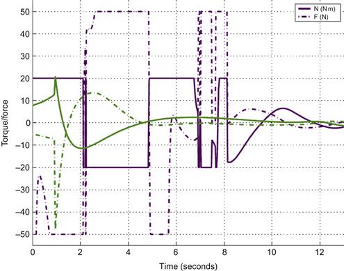
Figure 13.6 Control inputs (force and torque) for the dynamic and constrained kinematic stabilizing control. Source: Reprinted from Ref. [5], with permission from Institute of Electrical and Electronic Engineers.
When the force and torque are constrained, the system cannot track the reference velocities provided by the kinematic controller.
The invariant manifold controllers in Eqs. (6.117a) and (6.117b) for the double integrator (kinematic) WMR model and Eq. (6.130b) for the extended Brockett integrator (full kinematic and dynamic) model were also simulated [6]. Figure 13.7A and B shows the time performance of the kinematic controller in Eqs. (6.117a) and (6.117b) with ![]() , and
, and ![]() , sampling period
, sampling period ![]() , and control gains
, and control gains ![]() . The very quick convergence of
. The very quick convergence of ![]() , and
, and ![]() to zero is easily seen.
to zero is easily seen.
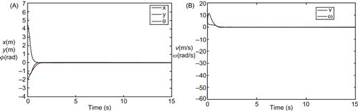
Figure 13.7 (A,B) Performance of the kinematic controller (6.117). (A) Trajectories of the states ![]() , and
, and ![]() . (B) Time evolution of linear velocity
. (B) Time evolution of linear velocity ![]() and angular velocity
and angular velocity ![]() . Source: Reprinted from Ref. [6], with permission from Institute of Electrical and Electronic Engineers.
. Source: Reprinted from Ref. [6], with permission from Institute of Electrical and Electronic Engineers.
The performance of the full dynamic controller (6.130b) was studied for the case where ![]()
![]()
![]()
![]()
![]()
![]()
![]() , and
, and ![]() . The physical parameters of the WMR used are
. The physical parameters of the WMR used are ![]() ,
, ![]()
![]() , and
, and ![]() . A slightly better performance was observed.
. A slightly better performance was observed.
13.6 Sliding Mode Fuzzy Logic Control
Here, some simulation results will be provided for the reduced complexity sliding mode fuzzy logic controller (RC-SMFLC) (8.39) [7,8]:
![]()
The uncertainty in the robot system lies in the variation of slopes ![]() . The robot may mount an uphill slope
. The robot may mount an uphill slope ![]() or go down a downhill slope
or go down a downhill slope ![]() , where both the magnitude and the sign of the slope are unknown and time varying.
, where both the magnitude and the sign of the slope are unknown and time varying.
The case of moving on an uphill was first considered. The fuzzy controller imitates the action of a human driver. If the slope increases, then the driver has to press more the acceleration pedal to maintain the velocity at the desired value, by compensating the increased effect of the gravitational term ![]() . If the robot acceleration exceeds the desired value, the pressure on the acceleration must be reduced. These “increase–decrease” acceleration actions, with gradually reducing amplitude, continue until the desired action is reached. The operation of the RC-SMFLC controller is similar when the robot moves on a downhill slope. Figure 13.8 shows the velocity fluctuation and the corresponding robot trajectory for a robot moving on an uphill with slope varying between 5% and 10%. The desired velocity was 4.2 m/s. Figure 13.9 shows the results of the robot when the robot descends a downhill with slope in the interval
. If the robot acceleration exceeds the desired value, the pressure on the acceleration must be reduced. These “increase–decrease” acceleration actions, with gradually reducing amplitude, continue until the desired action is reached. The operation of the RC-SMFLC controller is similar when the robot moves on a downhill slope. Figure 13.8 shows the velocity fluctuation and the corresponding robot trajectory for a robot moving on an uphill with slope varying between 5% and 10%. The desired velocity was 4.2 m/s. Figure 13.9 shows the results of the robot when the robot descends a downhill with slope in the interval ![]() .
.
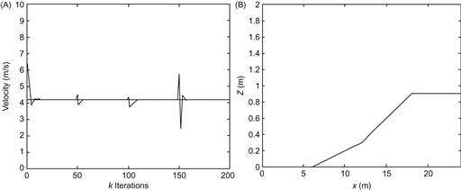
Figure 13.8 Robot performance ascending an uphill of uncertain slope. (A) Velocity fluctuation and (B) robot trajectory. Source: Reprinted from Ref. [7], with permission from Elsevier Science Ltd.
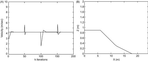
Figure 13.9 Robot performance descending a downhill of uncertain slope. (A) Velocity fluctuation and (B) robot trajectory. Source: Reprinted from Ref. [7], with permission from Elsevier Science Ltd.
The RC-SMFLC controller was also tested in the car-parking problem at a certain position of the uphill slope (here, at ![]() ), which is in the middle of the uphill slope. Clearly, this is a simplified form of the backing up control of a truck on an uphill slope, which is a difficult task for all but the most skilled drivers. To achieve backing up the desired position, the driver has to attempt backing, move forward, back again, go forward again, and so on. Figure 13.10 shows the performance of the position controller when the robot mounts an uphill (Figure 13.10A and B) and when the robot goes down a downhill slope (Figure 13.10C and D).
), which is in the middle of the uphill slope. Clearly, this is a simplified form of the backing up control of a truck on an uphill slope, which is a difficult task for all but the most skilled drivers. To achieve backing up the desired position, the driver has to attempt backing, move forward, back again, go forward again, and so on. Figure 13.10 shows the performance of the position controller when the robot mounts an uphill (Figure 13.10A and B) and when the robot goes down a downhill slope (Figure 13.10C and D).
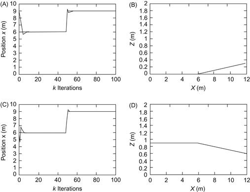
Figure 13.10 Control of the robot position on an uphill or downhill ![]() slope. (A) Uphill position evolution. (B) Robot trajectory corresponding to (A). (C) Downhill position evolution. (D) Robot trajectory corresponding to (C). Source: Reprinted from Ref. [7], with permission from Elsevier Science Ltd.
slope. (A) Uphill position evolution. (B) Robot trajectory corresponding to (A). (C) Downhill position evolution. (D) Robot trajectory corresponding to (C). Source: Reprinted from Ref. [7], with permission from Elsevier Science Ltd.
13.7 Vision-Based Control
Here, a number of simulation studies carried out using vision-based controllers will be presented [9–11].
13.7.1 Leader–Follower Control
First, some experimental results, obtained by the vision-based leader–follower tracking controller in Eqs. (9.75a) and (9.75b), with the linear velocity being estimated by Eq. (9.66), will be given [9]. These results were obtained for two Pioneer 2DX mobile robots, one following the other (Figure 13.11). The system hardware involved a frame grabber PXC200 in the vision part, which allowed image capturing by a SONY-EV-D30 camera mounted on the follower robot, and an image processor in charge of the calculation of the control actions (Pentium II-400 MHzPC).

Figure 13.12 shows the evolution of the distance to the leader. The task of the follower was to follow the leader robot maintaining a desired distance ![]() and an angle
and an angle ![]() . The desired control gains used are
. The desired control gains used are ![]() and
and ![]() , and the values of
, and the values of ![]() and
and ![]() were
were ![]() and
and ![]() .
.

Figure 13.13 shows the time profiles of the angles ![]() and
and ![]() , the control signals
, the control signals ![]() and
and ![]() of the follower robot, the estimated velocity of the leader, and the trajectory of the follower robot.
of the follower robot, the estimated velocity of the leader, and the trajectory of the follower robot.

Figure 13.13 Performance of the leader–follower visual controller. (A) Angles ![]() and
and ![]() . (B) Control signals
. (B) Control signals ![]() and
and ![]() . (C) Estimated velocity of the leader robot. (D) Trajectory of the follower robot. Source: Courtesy of R. Carelli.
. (C) Estimated velocity of the leader robot. (D) Trajectory of the follower robot. Source: Courtesy of R. Carelli.
From Figures 13.12 and 13.13 we see that the visual control scheme with variable gains according to Eq. (9.75c) assures the achievement of the desired overall objectives, while avoiding possible control saturation.
13.7.2 Coordinated Open/Closed-Loop Control
Second, some results obtained using the coordinated hybrid open/closed-loop controller of Example 10.2 will be given for a mobile manipulator [10]. The MM consists of a differential drive mobile platform and a 3-DOF manipulator. The manipulator Jacobian is found analogously to the 2-DOF manipulator, by adding to Eq. (10.10) an extra term to each element of ![]() corresponding to the third link (e.g.,
corresponding to the third link (e.g., ![]() is equal to
is equal to ![]() ). The link lengths used in the simulation are
). The link lengths used in the simulation are ![]()
![]() and
and ![]() . To maximize the manipulability index
. To maximize the manipulability index ![]() of the manipulator, its desired configuration was selected as
of the manipulator, its desired configuration was selected as ![]() . The kinematic model of the MM from the input velocities to the variation rates of the features is given in Eq. (10.62). The combination of controllers (10.63) and (10.64) for the feedback controller part was used with
. The kinematic model of the MM from the input velocities to the variation rates of the features is given in Eq. (10.62). The combination of controllers (10.63) and (10.64) for the feedback controller part was used with ![]() , being given by Eq. (10.66). The hybrid (open-loop/closed-loop) controller scheme (10.68) with parameters
, being given by Eq. (10.66). The hybrid (open-loop/closed-loop) controller scheme (10.68) with parameters ![]() , and
, and ![]() was used (see Eqs. (10.65) and (10.67)). The times
was used (see Eqs. (10.65) and (10.67)). The times ![]() and
and ![]() for the open-loop controller (10.71) were selected as
for the open-loop controller (10.71) were selected as ![]() and
and ![]() . Three landmarks
. Three landmarks ![]() , that is,
, that is, ![]() ,
, ![]() , and
, and ![]() , were used. The initial pose of the mobile platform was at the origin, and the manipulator’s initial configuration was selected close to the desired configuration. Figure 13.14 shows the features’ camera measurement errors
, were used. The initial pose of the mobile platform was at the origin, and the manipulator’s initial configuration was selected close to the desired configuration. Figure 13.14 shows the features’ camera measurement errors ![]() , the mobile base pose errors
, the mobile base pose errors ![]() , the mobile platform
, the mobile platform ![]() trajectory, and the platform’s control inputs
trajectory, and the platform’s control inputs ![]() and
and ![]() . The manipulability index value during the closed-loop control phase was
. The manipulability index value during the closed-loop control phase was ![]() , but it was sharply decreasing during the open-loop control phase. The camera measurement errors
, but it was sharply decreasing during the open-loop control phase. The camera measurement errors ![]() were strictly decreasing during the closed-loop control phase but remained constant during the open-loop control phase.
were strictly decreasing during the closed-loop control phase but remained constant during the open-loop control phase.

Figure 13.14 Performance of the coordinated hybrid visual controller of the MM. (A) Feature camera measurement errors. (B) Mobile platform pose errors. (C) Mobile Cartesian space trajectory. (D) Mobile platform’s control inputs ![]() and
and ![]() , which, in order to avoid the occurrence of limit cycles (due to the open-loop action), were applied only when the platform’s pose errors were larger than a selected threshold. Source: Reprinted from Ref. [10], with permission from Institute of Electrical and Electronic Engineers.
, which, in order to avoid the occurrence of limit cycles (due to the open-loop action), were applied only when the platform’s pose errors were larger than a selected threshold. Source: Reprinted from Ref. [10], with permission from Institute of Electrical and Electronic Engineers.
Finally, some results obtained using a full-state image-based controller for the simultaneous mobile platform and end effector (camera) pose stabilization are depicted in Figure 13.15. This controller was designed via a merging of the results of Sections 9.2, 9.4, 9.5, and 10.3, as described in Section 10.5. The distance ![]() of the target
of the target ![]() along the
along the ![]() -axis of the world coordinate frame was selected as
-axis of the world coordinate frame was selected as ![]() (see Figure 9.4), the camera focal length is
(see Figure 9.4), the camera focal length is ![]() , and the manipulator’s link lengths are
, and the manipulator’s link lengths are ![]() and
and ![]() [11].
[11].

Figure 13.15 (A) Platform ![]() trajectory from an initial to a final pose. (B) Control inputs
trajectory from an initial to a final pose. (B) Control inputs ![]() profiles. Source: Reprinted from Ref. [11], with permission from Springer Science+Business BV.
profiles. Source: Reprinted from Ref. [11], with permission from Springer Science+Business BV.
13.7.3 Omnidirectional Vision-Based Control
Experimental results through the two-step visual tracking control procedure of Section 9.9.3 were derived in Ref. [12] using a synchro-drive WMR and a PD controller:
![]()
where ![]() is the target’s feature error vector. The visual control loops worked at a rate of 33 ms without any frame loss, with the execution controller running at a rate of 7.5 ms. Originally, the target was at a distance 1 m from the robot, and then moved away along a straight path by 60 cm. Figure 13.16A shows a snapshot of the image acquired with the omnivision system, Figure 13.16B shows the robot and the target to be followed, and Figure 13.16C shows the evolution of the error signal in pixels. When the target stopped moving, the error was about ±2 pixels.
is the target’s feature error vector. The visual control loops worked at a rate of 33 ms without any frame loss, with the execution controller running at a rate of 7.5 ms. Originally, the target was at a distance 1 m from the robot, and then moved away along a straight path by 60 cm. Figure 13.16A shows a snapshot of the image acquired with the omnivision system, Figure 13.16B shows the robot and the target to be followed, and Figure 13.16C shows the evolution of the error signal in pixels. When the target stopped moving, the error was about ±2 pixels.

Figure 13.16 (A) Omnidirectional image showing the robot and target. (B) The robot and target. (C) Error signal. The robot started its movement at iteration 125. Source: Courtesy of J. Okamoto Jr [12].
We will now present a method and some experimental results derived for a car-like WMR:
![]()
using a calibrated catadioptric vision system, modeled as shown in Figure 9.26, in which case, ![]() , and:
, and:
![]()
where ![]() is given in Eq. (9.121b). The coordinate frame
is given in Eq. (9.121b). The coordinate frame ![]() attached to the robot is assumed to coincide with the mirror frame
attached to the robot is assumed to coincide with the mirror frame ![]() which implies that the camera frame and the WMR are subjected to identical kinematic constraints (Figure 13.17A).
which implies that the camera frame and the WMR are subjected to identical kinematic constraints (Figure 13.17A).
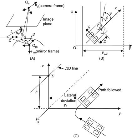
Figure 13.17 (A) A 3D line ![]() is projected into a conic in the image plane. (B) Variables and parameters of the robot and the problem. (C) Pictorial representation of the task to be performed. Source: Adapted from Refs. [13,14].
is projected into a conic in the image plane. (B) Variables and parameters of the robot and the problem. (C) Pictorial representation of the task to be performed. Source: Adapted from Refs. [13,14].
The problem is to drive the x-axis of the WMR (control) frame parallel to a given 3D straight line ![]() , while keeping a desired constant distance
, while keeping a desired constant distance ![]() to the line (Figure 13.17B and C) [13]. The line
to the line (Figure 13.17B and C) [13]. The line ![]() is specified by the position vector of a point
is specified by the position vector of a point ![]() on the line and its cross-product with the direction vector
on the line and its cross-product with the direction vector ![]() of the line, that is,
of the line, that is, ![]() in the mirror frame. Defining the vector
in the mirror frame. Defining the vector ![]() , the line
, the line ![]() is expressed in the so-called Plücker coordinates
is expressed in the so-called Plücker coordinates ![]() with
with ![]() . Let
. Let ![]() be the intersection between the interpretation plane
be the intersection between the interpretation plane ![]() (defined by the line
(defined by the line ![]() and the mirror focal point
and the mirror focal point ![]() ) and the mirror surface. Clearly,
) and the mirror surface. Clearly, ![]() is the line’s projection in the mirror surface. The projection
is the line’s projection in the mirror surface. The projection ![]() of the line
of the line ![]() in the catadioptric image plane is obtained using the relation
in the catadioptric image plane is obtained using the relation ![]() , where
, where ![]() is an arbitrary point
is an arbitrary point ![]() on
on ![]() , and:
, and:
![]()
which expresses the fact that ![]() is orthogonal to the interpretation plane. Inverting the relation
is orthogonal to the interpretation plane. Inverting the relation ![]() , we get:
, we get:
![]()
where:

with:

Introducing the above expression for ![]() into the condition
into the condition ![]() , we get:
, we get:

which after some algebraic manipulation can be written in the standard quadratic form [13,14]:
where ![]() in the general case, and
in the general case, and ![]() in the parabolic mirror–orthographic camera case. In expanded form, the above quadratic equation can be expressed in the following normalized form:
in the parabolic mirror–orthographic camera case. In expanded form, the above quadratic equation can be expressed in the following normalized form:
![]()
where ![]() is a scaling factor. The nondegenerate case
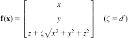
is a scaling factor. The nondegenerate case ![]() is considered. The state of the WMR (and camera) is:
is considered. The state of the WMR (and camera) is:
![]()
where ![]() are the world coordinates of the camera and
are the world coordinates of the camera and ![]() the angular deviation with respect to the straight line. The task is achieved when the lateral deviation
the angular deviation with respect to the straight line. The task is achieved when the lateral deviation ![]() is equal to the desired deviation
is equal to the desired deviation ![]() , and the angular deviation is zero. These deviations are expressed in terms of image features as [14]:
, and the angular deviation is zero. These deviations are expressed in terms of image features as [14]:
![]()
assuming ![]() and
and ![]() (i.e., that the line
(i.e., that the line ![]() does not lie on the
does not lie on the ![]() plane of the camera frame
plane of the camera frame ![]() , and the x-axis of the mirror is not perpendicular to the line
, and the x-axis of the mirror is not perpendicular to the line ![]() ). The parameter
). The parameter ![]() is shown in Figure 13.17C. Choosing
is shown in Figure 13.17C. Choosing ![]() in the WMR chained model we get:
in the WMR chained model we get:
![]()
Further, choosing ![]() we have
we have ![]() , and so
, and so ![]() (for
(for ![]() ). Now:
). Now:
![]()
Dividing the equations of the chained model by ![]() we get:
we get:
![]()
where ![]() . Selecting the state feedback controller
. Selecting the state feedback controller ![]() for the above linear system as:
for the above linear system as:
![]()
we get the closed-loop error (deviation) equation:
![]()
Therefore, selecting proper values for the gains ![]() and
and ![]() assures that
assures that ![]() and
and ![]() , as
, as ![]() (with desired convergence rates) independently of the longitudinal velocity as long as
(with desired convergence rates) independently of the longitudinal velocity as long as ![]() . From the relations
. From the relations ![]() and
and ![]() , it follows that also
, it follows that also ![]() and
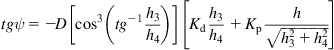
and ![]() . The expression for the feedback control steering angle
. The expression for the feedback control steering angle ![]() is found from:
is found from:
that is:
In terms of the measured features ![]() and
and ![]() , this controller is expressed as:
, this controller is expressed as:
The parameter ![]() is obtained from proper measurement.
is obtained from proper measurement.
The above controller was tested by simulation for both a paracatadioptric sensor (parabolic mirror plus orthographic camera) and a hypercatadioptric sensor (hyperbolic mirror plus perspective camera) [13,14]. In the first case, the image of a line is a circle and in the second case is a part of a conic. Figure 13.18A and B shows the line configuration and actual robot trajectory in the world coordinate frame, and the profiles of the lateral and angular deviations provided by the simulation.
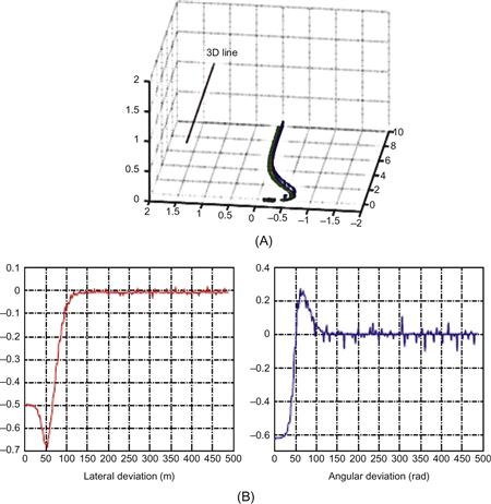
Figure 13.18 Omnidirectional visual servoing results with ![]() . (A) Desired line and actual robot trajectory, (B) Evolution of lateral and angular deviations. Reprinted from [13], with permission from Institute of Electrical and Electronic Engineers.
. (A) Desired line and actual robot trajectory, (B) Evolution of lateral and angular deviations. Reprinted from [13], with permission from Institute of Electrical and Electronic Engineers.
Similar results were reported for the case of hypercatadioptric system [13].
13.8 Sliding Mode Control of Omnidirectional Mobile Robot
Here, some simulation results for the omnidirectional mobile manipulator of Section 10.3.4, with three links ![]() will be given. The sliding mode controller (10.53b) has been applied, replacing the switching term
will be given. The sliding mode controller (10.53b) has been applied, replacing the switching term ![]() by the saturation function approximation
by the saturation function approximation ![]() as described in Section 7.2.2. The parameter values of the MM are given in Table 13.1. The masses and moments of inertia were assumed to contain uncertainties in intervals between
as described in Section 7.2.2. The parameter values of the MM are given in Table 13.1. The masses and moments of inertia were assumed to contain uncertainties in intervals between ![]() and
and ![]() of their nominal values (Table 13.1). The simulation results were obtained using the extreme values as the real ones, and the mean values of the true and extreme values as the estimated values for the computation of the control signals.
of their nominal values (Table 13.1). The simulation results were obtained using the extreme values as the real ones, and the mean values of the true and extreme values as the estimated values for the computation of the control signals.
Table 13.1
Parameter Values of the Robotic Manipulator
| Physical Variable | True Value | Extreme Uncertain Values |
| Mass of each wheel | 0.5 kg | 0.525 kg (+5%) |
| Radius of each wheel | 0.0245 m | 0.0245 m |
| Mass of the platform | 30 kg | 33 kg (+10%) |
| Wheel distance from the platform COG | 0.178 m | 0.178 m |
| Platform moment of inertia with respect to axis z | 0.93750 kg m2 | 0.98435 kg m2 (+5%) |
| Mass of link 1 | 1.25 kg | 1.375 kg (+10%) |
| Length of link 1 | 0.11 m | 0.11 m |
| Link 1 moment of inertia with respect to axis x | 0.01004 kg m2 | 0.010542 kg m2 (+5%) |
| Mass of link 2 | 4.17 kg | 5.421 kg (+30%) |
| Length of link 2 | 0.5 m | 0.5 m |
| Position of link’s COG along its axis | 0.25 m | 0.25 m |
| Link 2 moment of inertia with respect to axis x | 0.34972 kg m2 | 0.367206 kg m2 (+5%) |
| Link-2 moment of inertia with respect to axis z | 0.00445 kg m2 | 0.0046725 kg m2 (+5%) |
| Mass of link 3 | 0.83 kg | 1.0790 kg (+30%) |
| Length of link 3 | 0.10 m | 0.10 m |
| Position of link’s 3 COG along its axis | 0.05 m | 0.05 m |
| Link 3 moment of inertia with respect to axis x | 0.00321 kg m2 | 0.0033705 kg m2 (+5%) |
| Link 3 moment of inertia with respect to axis z | 0.00089 kg m2 | 0.0009345 kg m2 (+5%) |
| Linear friction coefficient for all rotating joints | 0.1 N m s | 0.13 (+30%) |
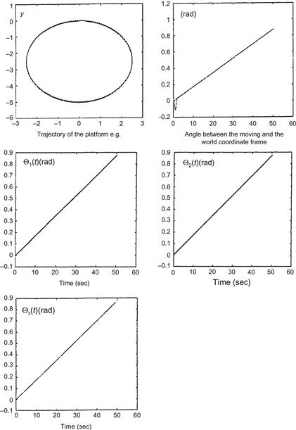
1. Linear desired trajectory of the platform’s center of gravity
2. Circular desired trajectory of the platform’s center of gravity
In both cases, an angular platform velocity of ![]() with respect to the world coordinate frame was applied. For the joint variables, a ramp reference was used. The results obtained via simulation are shown in Figures 13.19 and 13.20 [15]. The results obtained using the exact values in the computed torque method showed that the sliding mode controller (with the
with respect to the world coordinate frame was applied. For the joint variables, a ramp reference was used. The results obtained via simulation are shown in Figures 13.19 and 13.20 [15]. The results obtained using the exact values in the computed torque method showed that the sliding mode controller (with the ![]() function approximation) can indeed face large parametric uncertainties and follow the desired trajectories successfully.
function approximation) can indeed face large parametric uncertainties and follow the desired trajectories successfully.

13.9 Control of Differential Drive Mobile Manipulator
13.9.1 Computed Torque Control
In the following discussion, some simulation results obtained by the application of the computed torque controller ((10.49a) and (10.49b)) to the 5-DOF MM of Figure 10.8 will be provided. The parameters of the MM are given in Table 13.2 [16].

The desired performance specifications for the error dynamics were selected to be ![]() and
and ![]() (settling time
(settling time ![]() ). Then, the gain matrices
). Then, the gain matrices ![]() and
and ![]() in Eq. (10.49b) are:
in Eq. (10.49b) are:
![]()
The control torques of the left and right wheel and the forearms and upper arms that result with the above gains are shown in Figure 13.21A and B. The desired trajectories of the manipulator front point ![]() and the end effector tip E are shown in Figure 13.21C. The corresponding actual animated paths are shown in Figure 13.21D.
and the end effector tip E are shown in Figure 13.21C. The corresponding actual animated paths are shown in Figure 13.21D.

Figure 13.21 (A) Torques of driving wheels. (B) Forearm and upper arm torques. (C) Desired paths of the platform’s front point ![]() and end effector. (D) Actual animated paths of the platform and the end effector. Source: Courtesy of E. Papadopoulos [16].
and end effector. (D) Actual animated paths of the platform and the end effector. Source: Courtesy of E. Papadopoulos [16].
13.9.2 Control with Maximum Manipulability
Here, we will present a few representative simulation results obtained in Refs. [17,18] for the MM of Figure 10.11. The platform parameters used are those of the LABMATE platform (Transition Research Corporation) and the manipulator parameters are ![]() .
.
The center of gravity of each link was assumed to be at the midpoint of the link, and the sampling period was set to ![]() .
.
13.9.2.1 Problem (a)
The controller ((10.55a) and (10.55b)) was applied leading to the decoupled system (10.55c). This system was controlled by a diagonal (decoupled) PD tracking controller for the desired specifications ![]() and
and ![]() . The overdamping
. The overdamping ![]() was selected to match the slow response of the platform. The velocity along the path was assumed constant.
was selected to match the slow response of the platform. The velocity along the path was assumed constant.
Figure 13.22A and B shows the desired and actual trajectories of the wheel midpoint ![]() and the reference (end effector) point for the case where the desired path was a straight line 45° from the x-axis. The notch on one side of each square platform shows the forward direction of motion.
and the reference (end effector) point for the case where the desired path was a straight line 45° from the x-axis. The notch on one side of each square platform shows the forward direction of motion.

Figure 13.22 (A) Trajectory of the point ![]() for the
for the ![]() straight path. (B) Desired and actual trajectories of the end effector for the path (A). Source: Reprinted from Ref. [17], with permission from Institute of Electrical and Electronic Engineers.
straight path. (B) Desired and actual trajectories of the end effector for the path (A). Source: Reprinted from Ref. [17], with permission from Institute of Electrical and Electronic Engineers.
The manipulability was kept at its maximum except for the initial maneuvering period of the platform (about 5 s).
13.9.2.2 Problem (b)
Four cases were simulated with or without compensation as follows:
Case 1: Compensation of both the arm and the platform
Case 2: Compensation of the arm only
Figure 13.23A and B shows representative results for the case of a circular desired path.
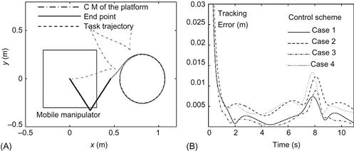
Figure 13.23 (A) Trajectories of COG and end point, and task trajectory. (B) Corresponding tracking errors. Source: Reprinted from Ref. [18], with permission from Electrical and Electronic Engineers.
13.10 Integrated Global and Local Fuzzy Logic-Based Path Planner
Here, simulation results of an integrated navigation (global planning and local/reactive planning) scheme for omnidirectional robots using fuzzy logic rules will be presented [19,20]. A description of this two-level model (Figure 13.24) will be first provided.
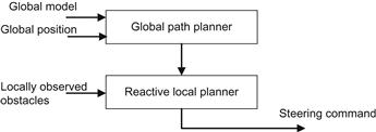
The global path planner is based on the potential field method and provides a nominal path between the current configuration of the robot and its goal. The local reactive planner generates the appropriate commands for the robot actuators to follow the global path as close as possible, while reacting in real time to unexpected events by locally adapting the robot’s movements, so as to avoid collision with unpredicted or moving obstacles. This local planner consists of two separate fuzzy controllers for path following and obstacle avoidance (Figure 13.25).

The inputs to the local planner are the path provided by the global path planner and the locally observed obstacles. The output is the steering command for the actuators of the robot. This steering command is a weighed sum of the outputs of the two fuzzy controllers as shown in Figure 13.26.
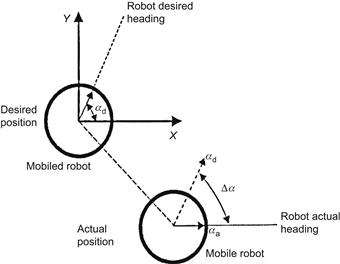
Figure 13.26 Actual and desired configurations of the mobile robot. ![]() denotes the desired heading,
denotes the desired heading, ![]() denotes the actual heading, and
denotes the actual heading, and ![]() denotes the difference between the actual and the desired heading of the mobile robot.
denotes the difference between the actual and the desired heading of the mobile robot.
The purpose of the fuzzy path following module is to generate the appropriate commands for the actuators of the robot, so as to follow the global path as close as possible, while minimizing the error between the current heading of the robot and the desired one, obtained from the path calculated by the global planner (Figure 13.26). It has one input, the difference ![]() between the desired and the actual heading of the robot, and one output, a steering command
between the desired and the actual heading of the robot, and one output, a steering command ![]() .
.
The fuzzy module/controller is based on the Takagi–Sugeno method.1 The input space is partitioned by fuzzy sets as shown in Figure 13.27. Here, asymmetrical triangular and trapezoidal functions which allow a fast computation, essential under real-time conditions, are utilized to describe each fuzzy set (see Eqs. (13.1–13.3)) below.
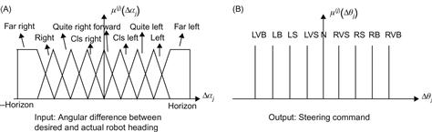
Figure 13.27 Fuzzy sets for the path following unit. (A) Input ![]() : angular difference between desired and actual robot heading. (B) Output
: angular difference between desired and actual robot heading. (B) Output ![]() : steering command (note that the output is not partitioned into fuzzy sets, but consists of crisp values).
: steering command (note that the output is not partitioned into fuzzy sets, but consists of crisp values).
To calculate the fuzzy intersection, the product operator is employed. The final output of the unit is given by a weighted average over all rules (see Eq. (13.5) and Figure 13.27).
Intuitively, the rules for the path following module can be written as sentences with one antecedent and one conclusion (see Eq. (13.4)). As described in Example 8.3, this structure lends itself to a tabular representation. This representation is called fuzzy associative matrix (FAM) and represents the prior knowledge of the problem domain (Table 13.3).

The symbols in Table 13.3 have the following meaning: LVB, left very big; LB, left big; LS, left small; LVS, left very small; N, neutral (zero); RVB, right very big; RB, right big; RS, right small; RVS, right very small.
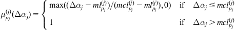
The rows represent the fuzzy (linguistic) values of the distance to an obstacle, the columns are the fuzzy values of angles to the goal, and the elements of the matrix are the torque commands of the motor. The tools of fuzzy logic allow us to translate this intuitive knowledge into a control system. The fuzzy set ![]() is described by asymmetrical triangular and trapezoidal functions. Defining the parameters
is described by asymmetrical triangular and trapezoidal functions. Defining the parameters ![]() and
and ![]() as the
as the ![]() -coordinates of the left and right zero crossing, respectively, and
-coordinates of the left and right zero crossing, respectively, and ![]() and
and ![]() as the
as the ![]() -coordinates of the left and right side of the trapezoid’s plateau, the trapezoidal functions can be written as:
-coordinates of the left and right side of the trapezoid’s plateau, the trapezoidal functions can be written as:
 (13.1)
with ![]() . Triangular functions can be achieved by setting
. Triangular functions can be achieved by setting ![]() . On the left and right side of the interval, the functions are continued as constant values of magnitude 1, that is:
. On the left and right side of the interval, the functions are continued as constant values of magnitude 1, that is:
 (13.2)
and
 (13.3)
The fuzzy set ![]() is associated with linguistic terms
is associated with linguistic terms ![]() . Thus, for the mobile robot, the linguistic control rules
. Thus, for the mobile robot, the linguistic control rules ![]() , which constitute the rule base, can be defined as:
, which constitute the rule base, can be defined as:
![]() (13.4)
(13.4)
Finally, the output of the unit is given by the weighted average over all rules:
![]() (13.5)
(13.5)
Equation (13.4) together with Eq. (13.5) defines how to translate the intuitive knowledge reflected in the FAM into a fuzzy rule base. The details of this translation can be modified by changing the number of fuzzy sets, the shape of the sets (by choosing the parameters ![]() ,
, ![]() ) as well as the value
) as well as the value ![]() of each of the rules in Eq. (13.5). As an example, in this application, the number of fuzzy sets that fuzzifies the angular difference in heading
of each of the rules in Eq. (13.5). As an example, in this application, the number of fuzzy sets that fuzzifies the angular difference in heading ![]() is chosen to be nine. All the other parameters were refined by trial and error. The fuzzy-based obstacle avoidance unit, which controls the mobile robot, has three principal inputs:
is chosen to be nine. All the other parameters were refined by trial and error. The fuzzy-based obstacle avoidance unit, which controls the mobile robot, has three principal inputs:
1. The distance ![]() between the robot and the nearest obstacle.
between the robot and the nearest obstacle.
2. The angle ![]() between the robot and the nearest obstacle.
between the robot and the nearest obstacle.
3. The angle ![]() between the robot’s direction and the straight line connecting the current position of the robot and the goal configuration, where
between the robot’s direction and the straight line connecting the current position of the robot and the goal configuration, where ![]() is the direction of the straight line connecting the robot’s current position and the goal position, and
is the direction of the straight line connecting the robot’s current position and the goal position, and ![]() is the current direction of the robot (Figure 13.28).
is the current direction of the robot (Figure 13.28).
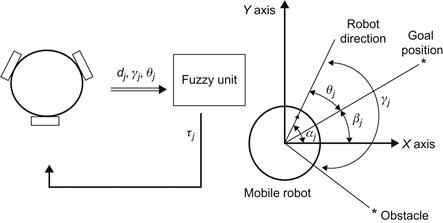
Figure 13.28 The omnidirectional mobile robot connected to the corresponding fuzzy-based obstacle avoidance unit. This unit receives via an input the angle ![]() between the robot’s direction and the straight line connecting the current position of the robot and the goal configuration, and the distance and the angle of the nearest obstacle
between the robot’s direction and the straight line connecting the current position of the robot and the goal configuration, and the distance and the angle of the nearest obstacle ![]() . The output variable of the unit is the motor command
. The output variable of the unit is the motor command ![]() .
.
The output variable of the unit is the motor torque command ![]() . All these variables can be positive or negative, that is, they do not only inform about the magnitude but also about the sign of displacement relative to the robot left or right. The motor command which can be interpreted as an actuation for the robot’s direction motors is fed to the mobile platform at each iteration. It is assumed that the robot is moving with constant velocity, and no attempt is being made to control it.
. All these variables can be positive or negative, that is, they do not only inform about the magnitude but also about the sign of displacement relative to the robot left or right. The motor command which can be interpreted as an actuation for the robot’s direction motors is fed to the mobile platform at each iteration. It is assumed that the robot is moving with constant velocity, and no attempt is being made to control it.
For the calculation of the distance, the only obstacles considered are those which fall into a bounded area surrounding the robot and moving along with it. In this implementation, this area is chosen to be a cylindrical volume around the mobile platform and reaches up to a predefined horizon. This area can be seen as a simplified model for the space scanned by ranging sensors (e.g., ultrasonic sensors) attached to the sides of the robot. Besides an input from ultrasonic sensors, a camera can also be used to acquire the environment. Mobile robots are usually equipped with a pan/tilt platform where a camera is mounted. This camera can also be utilized. If no obstacle is detected inside the scan area, the fuzzy unit is informed of an obstacle in the far distance.
13.10.1 Experimental Results
The functioning of the proposed system, applied to an omnidirectional mobile robot, was evaluated through simulations using Matlab. In all cases, the proposed planner provided the mobile robot with a collision-free path to the goal position. Simulation results, obtained in three different working scenarios, are shown inFigure 13.29 [20].
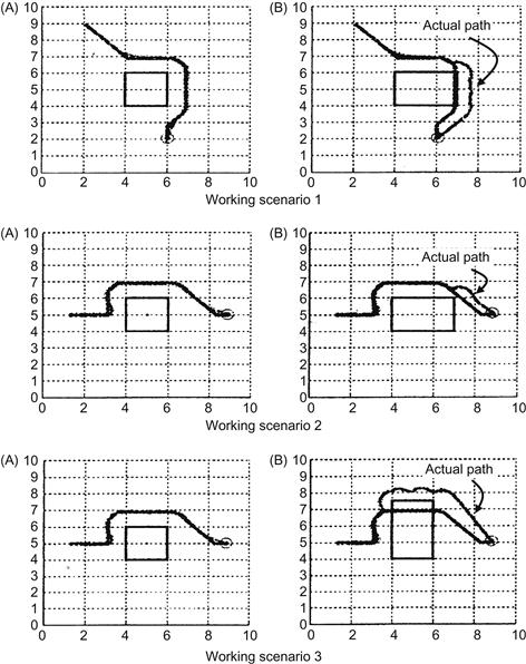
Figure 13.29 Three scenarios of simulation results. (A) Actual path of the robot and the global path coincide since the world model was accurate. (B) Actual path of the robot is different from the path provided by the global path planner since the position/size of the obstacle was not very accurate or the obstacle moved to a new position.
The present two-level fuzzy global and local path planning control method can also be directly applied to fixed industrial robots [19], as well as to mobile manipulators.
13.11 Hybrid Fuzzy Neural Path Planning in Uncertain Environments
Here, a hybrid sensor-based mobile robot path planning algorithm in uncertain and unknown environments, with corresponding simulation results, will be presented [21]. The constraints and the solution style adopted are similar to those followed by a human decision maker when he (she) tries to solve a path planning problem of this type. The human does not know precisely the position of the goal, and so he (she) makes use of its direction, and the information he (she) gets about the distance, the shape of the obstacles, at their visible side, which is strongly fuzzy. The present path planning problem does not allow the use of the standard scheme “data input–processing–data output” since here there are some rules that do not depend on the input data but affect the output. Examples of such rules are as follows:
• The robot motion must be close as much as possible to the direction of the goal.
• If a movement direction has been selected, it is not advisable to change it without prior consideration, unless some other much better direction is brought to the robot’s attention.
• If the robot returns to a point that has been passed before, it should select an alternative route (direction) in order not to make endless loops and consequently reach a dead end.
For this reason, the robot path planning system should involve two subsystems, namely, a subsystem connected to the input, and a subsystem that is not connected to the input, but is modified by the output values. It seems to be convenient to use a fuzzy logic algorithm in the first subsystem (since the sensor measurements are fuzzy) and a neural model in the second subsystem for the rules that have to be adaptive. The general structure of such a system is shown in Figure 13.30.

Here, the subsystem II is implemented algorithmically, that is, without the use of neural network, but through a merging operation based on simple multiplication.
13.11.1 The Path Planning Algorithm
It will be assumed that the autonomous robot (represented by a point in the space) has to move from an initial position ![]() (start) to a final position
(start) to a final position ![]() (goal). The available data are measurements from the sensors about all required quantities. These measurements are obtained from the current position
(goal). The available data are measurements from the sensors about all required quantities. These measurements are obtained from the current position ![]() of the robot. The direction of the goal
of the robot. The direction of the goal ![]() , that is, the direction of the straight line
, that is, the direction of the straight line ![]() is also assumed to be measured, but the length (distance)
is also assumed to be measured, but the length (distance) ![]() is not measured. Then, the algorithm works as follows: we first define a coordinate frame attached to the robot system with Ox-axis the straight line
is not measured. Then, the algorithm works as follows: we first define a coordinate frame attached to the robot system with Ox-axis the straight line ![]() , and divide the space into
, and divide the space into ![]() directions with reference the
directions with reference the ![]() (or Ox) direction. Obviously, two consecutive directions have an angular distance of
(or Ox) direction. Obviously, two consecutive directions have an angular distance of ![]() degrees. It is convenient to select the number
degrees. It is convenient to select the number ![]() of directions such that the axes
of directions such that the axes ![]() , and
, and ![]() are involved in them. Now, from the sensors’ measurements and the fuzzy inference on the database, we determine and associate to each direction a priority. Then, we select the direction with the highest priority, and the new point
are involved in them. Now, from the sensors’ measurements and the fuzzy inference on the database, we determine and associate to each direction a priority. Then, we select the direction with the highest priority, and the new point ![]() is placed in this direction with
is placed in this direction with ![]() , where
, where ![]() is the step length that we select.
is the step length that we select.
On the basis of the above, the path planning algorithm is implemented by the following steps:
Step 1: Obtain the measurements from the position ![]() .
.
Step 2: Fuzzify the results of these measurements.
Step 3: Introduce the fuzzy results into the rules adopted.
Step 4: Determine a priority value for each direction.
Step 5: Multiply the above priority value by a given a priori weight for each direction.
Step 6: Determine the direction with the highest priority, move by a step length in this direction to find ![]() .
.
The fuzzy database contains suitable rules, the inputs of which are obtained from the sensors. The a priori knowledge used for the robot motion is expressed in the form of a weight for each direction, and there is no need to be determined each time from the knowledge base. For example, the direction from the current position to the goal must have the highest priority. Similarly, the directions that approach the goal must have higher priorities than the directions that depart from the goal. The representation of this a priori knowledge in the form of weights suggests the use of a neural network which accepts as inputs the priorities of the ![]() directions, and has as weights the weights of the a priori knowledge (Figure 13.30). These weights can be predetermined by trial and error work and can be updated periodically after a certain number of steps. In this way, we ensure the learning of the relationship between the a priori knowledge and the output of the fuzzy inference (not the learning of the a priori knowledge itself). An algorithm is also required to overcome the dead ends that may appear when a cycle occurs in which the weights of the a priori knowledge do not change. This algorithm varies from case to case. In the simulation example that follows, we used a fast algorithm for this purpose which runs over each cycle of the path planning algorithm.
directions, and has as weights the weights of the a priori knowledge (Figure 13.30). These weights can be predetermined by trial and error work and can be updated periodically after a certain number of steps. In this way, we ensure the learning of the relationship between the a priori knowledge and the output of the fuzzy inference (not the learning of the a priori knowledge itself). An algorithm is also required to overcome the dead ends that may appear when a cycle occurs in which the weights of the a priori knowledge do not change. This algorithm varies from case to case. In the simulation example that follows, we used a fast algorithm for this purpose which runs over each cycle of the path planning algorithm.
The present algorithm has a very general structure and can be used to any path planning problem in an unknown environment where optimality is not required. The algorithm needs only to have available the rules of the fuzzy database, the length ![]() of the motion step, and the number
of the motion step, and the number ![]() of the directions that are examined.
of the directions that are examined.
13.11.2 Simulation Results
The simulation robot path planning example was designed to have the following particular features:
• The distance ![]() from the point
from the point ![]() to some obstacle point (e.g., an obstacle or the room wall) is assumed to be measured by a sensor.
to some obstacle point (e.g., an obstacle or the room wall) is assumed to be measured by a sensor.
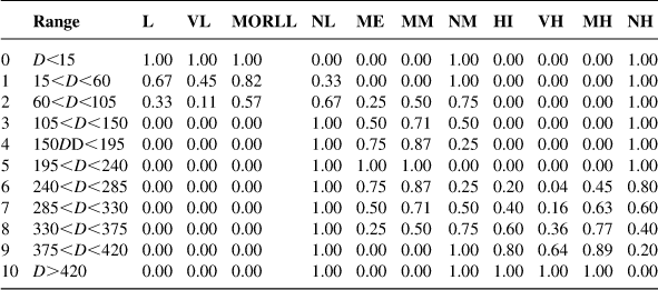
• The measurement results are quantized in 11 intervals and fuzzified as given in Table 13.4
The entries of this table are the values of membership functions ![]() of the distance in the various ranges
of the distance in the various ranges ![]() as distributed among the linguistic values L, VL, MORLL, NL, ME, MM, NM, HI, VH, MH, NH, and UN. The respective code of these values is described as follows: L, low; VL, very low; MORLL, more or less low; ME, medium; MM, more or less medium; NM, not medium; H, high; VH, very high; MH, more or less high; NH, not high; UN, unknown.
as distributed among the linguistic values L, VL, MORLL, NL, ME, MM, NM, HI, VH, MH, NH, and UN. The respective code of these values is described as follows: L, low; VL, very low; MORLL, more or less low; ME, medium; MM, more or less medium; NM, not medium; H, high; VH, very high; MH, more or less high; NH, not high; UN, unknown.
• The rules employed are the following:
R2=IF ![]() is medium, THEN
is medium, THEN ![]() is medium
is medium
where ![]() is the priority of the ith direction quantized in 11 intervals and fuzzified according to Table 13.4.
is the priority of the ith direction quantized in 11 intervals and fuzzified according to Table 13.4.
• The knowledge is represented by fuzzy matrices where Zadeh’s max-min inference rule is applied.
• The fuzzification is performed using the singleton method, and the defuzzification using the center of gravity method.
• The number of directions is selected to be ![]() and the step length to be
and the step length to be ![]() pixels.
pixels.
• The weights in the network selecting the maximum direction priority (i.e., the weights of the a priori knowledge) are predetermined as:
![]()
The robot environment used in the present example was obtained on a VGA640x480 screen. During the motion, the “mouse” was regarded as a moving obstacle. The results of four experiments with different starting and goal points are shown in Figure 13.31A–D [21].

13.12 Extended Kalman Filter-Based Mobile Robot SLAM
Here, some results obtained for the SLAM problem using EKFs will be presented (Section 12.8.2). The differential drive WMR SLAM problem of Example 12.3 (Figure 12.11) was solved using a global reference at the origin, which assures that the EKF is stable [22]. Actually, the robot and landmark covariance estimates were proved to be significantly reduced, and the actual robot path and landmark estimates showed a significant error reduction. This is shown in Figure 13.32 where the results are compared to the GPS measurements for two anchors located at (2.8953,−4.0353) and (9.9489, 6.9239).
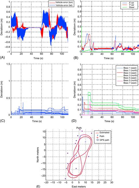
Figure 13.32 (A,B) EKF errors and covariance of the robot. (C,D) Landmark localization errors and covariance. (E) Robot path and landmark location estimates compared to GPS ground truth. Source: Courtesy of T.A. Vidal Calleja [22].
13.13 Particle Filter-Based SLAM for the Cooperation of Two Robots
Here, some results obtained by applying the particle filter approach of Section 12.8.4 to WMR SLAM for a pair of robots performing collaborative exploration will be presented [23,24]. The parameters ![]() used allow the modeling of the poses and uncertainties of the robots. The strategy for cooperative exploration of the two robots is to allow them to take turns moving such that at each time one robot is stationary and can be considered as a fixed reference point (Figure 13.33).
used allow the modeling of the poses and uncertainties of the robots. The strategy for cooperative exploration of the two robots is to allow them to take turns moving such that at each time one robot is stationary and can be considered as a fixed reference point (Figure 13.33).
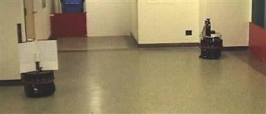
Figure 13.33 The two cooperating WMRs exploring one side of a room. Source: Reprinted from Ref. [24], with permission from Institute of Electrical and Electronic Engineers.
The positions of the two robots are estimated via the particle filter combining an open-loop estimate of odometry error with data from a range finder on one robot and a three-plane target mounted on top of the other robot.
13.13.1 Phase 1 Prediction
Here, the variable of interest is the pose ![]() of the moving robot. The robot motion is performed as a rotation followed by a translation. The rotation angle is equal to
of the moving robot. The robot motion is performed as a rotation followed by a translation. The rotation angle is equal to ![]() , where
, where ![]() , and the forward translation distance is
, and the forward translation distance is ![]() . If the starting pose is
. If the starting pose is ![]() , then the resulting pose is
, then the resulting pose is ![]() given by:
given by:
The rotation error (noise) ![]() due to odometric error is assumed to be a Gaussian process with mean value
due to odometric error is assumed to be a Gaussian process with mean value ![]() and standard deviation proportional to
and standard deviation proportional to ![]() , that is,
, that is, ![]() . The translation noise has two components: the first is related to the actual distance travelled (pure translation noise), and the second is due to changes in orientation during the forward translation. This component is called drift. The mean values
. The translation noise has two components: the first is related to the actual distance travelled (pure translation noise), and the second is due to changes in orientation during the forward translation. This component is called drift. The mean values ![]() and the standard deviations
and the standard deviations ![]() of these two components can be determined experimentally by discretizing the simulated motion in L steps. The standard deviations per step are equal to:
of these two components can be determined experimentally by discretizing the simulated motion in L steps. The standard deviations per step are equal to:
![]()
Therefore, the WMR stochastic prediction model is:
where ![]() , and
, and ![]() are Gaussian noises with mean values
are Gaussian noises with mean values ![]() and standard deviations
and standard deviations ![]() .
.
An experiment where the robot moved forward three times (horizontally to the right), rotated by ![]() , then moved forward three more times, after that rotated again by
, then moved forward three more times, after that rotated again by ![]() , and translated forward five times showed that the uncertainty grows without bound.
, and translated forward five times showed that the uncertainty grows without bound.
13.13.2 Phase 2 Update
After each motion, the robot range finder (RF) sensor sends a measurement vector ![]() , where
, where ![]() , and
, and ![]() are as shown in Figure 13.34.
are as shown in Figure 13.34.
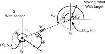
Figure 13.34 The range finder (RF) sensor mounted on the stationary robot (SR) observes the moving robot (MR) that carries the target. The tracker gives ![]() , and
, and ![]()
![]() . Source: Adapted from Ref. [24].
. Source: Adapted from Ref. [24].
The laser range finder can always detect at least two planes of the three-plane target from any position around the moving robot. The sensor output ![]() is given by:
is given by:

where ![]() is the pose of the moving robot and
is the pose of the moving robot and ![]() is the pose of the stationary robot,
is the pose of the stationary robot, ![]() and
and ![]() .
.
Using the sensor measurement ![]() , the weights are updated as shown in Eqs. (12.68b) and (12.69):
, the weights are updated as shown in Eqs. (12.68b) and (12.69):
where ![]() is the following Gaussian distribution:
is the following Gaussian distribution:

assuming that the processes ![]() , and
, and ![]() are statistically independent.
are statistically independent.
13.13.3 Phase 3 Resampling
When the effective sampling size ESS (see Eq. (12.70)) is less than the threshold ![]() , the particle population is resampled to eliminate (probabilistically) the ones with small weights.
, the particle population is resampled to eliminate (probabilistically) the ones with small weights.
13.13.4 Experimental Work
The mapping algorithm of the room is based on triangulation of free space by the two robots (see Section 12.6.3). The “sweep” of the space is performed using the line of visual contact of the two robots, that is, if the two robots can see each other, there is no obstacle in the space between them. If a robot is located at a corner (stationary) and the other moves along a wall (always without losing visual contact), then a triangle of free space is mapped. The environment is completely mapped by the robots using an online triangulation of the free space [23,24]. Figure 13.35 shows experimental results with two robots exploring the convex area of the corridors of a building. Both subfigures show a spatial integration of the particles during the full trajectory.
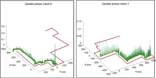
Figure 13.35 Convex area exploration by the two robots: (A) trajectory of robot 0; (B) trajectory of robot 1. The peak heights represent accuracy (the higher a peak the more accurate the estimation). Source: Reprinted from Ref. [24], with permission from Institute of Electrical and Electronic Engineers.
13.14 Neural Network Mobile Robot Control and Navigation
Here, simulation results will be presented concerning two problems:
1. Neural network-based mobile robot trajectory tracking
2. Neural network-based mobile robot obstacle avoiding navigation.
13.14.1 Trajectory Tracking
The general method of Section 8.5 was applied to a differential drive WMR using a PD velocity controller to train a multilayer perceptron (MLP), as shown in Figure 8.11. The PD teacher controller has the form:
![]()
where ![]() , and has been designed to guarantee exponential convergence of
, and has been designed to guarantee exponential convergence of ![]() to the desired trajectory
to the desired trajectory ![]() . The desired trajectory was generated by a reference (virtual) WMR so as to assure that it is compatible with the kinematic nonholonomic constraint of the robot under control. The gain matrix
. The desired trajectory was generated by a reference (virtual) WMR so as to assure that it is compatible with the kinematic nonholonomic constraint of the robot under control. The gain matrix ![]() was chosen such that:
was chosen such that:
![]()
A specific value of ![]() that assured good exponential trajectory convergence is
that assured good exponential trajectory convergence is ![]() , and was used in the experiment. A two-layer MLP NN was used with 10 nodes in the hidden layer and 1 node in the output layer. This NN was trained by the BP algorithm with input–output data the velocity
, and was used in the experiment. A two-layer MLP NN was used with 10 nodes in the hidden layer and 1 node in the output layer. This NN was trained by the BP algorithm with input–output data the velocity ![]() and the position
and the position ![]() , respectively. The structure of the neurocontroller is shown in Figure 13.36 [25].
, respectively. The structure of the neurocontroller is shown in Figure 13.36 [25].

Figure 13.36 WMR supervised tracking neurocontroller. Source: Adapted from Ref. [25].
In this scheme the NN, instead of learning explicit trajectories, is trained to learn the relationship between the linear velocity ![]() and the position error
and the position error ![]() . The learning rate is adjusted by the rule:
. The learning rate is adjusted by the rule:
![]()
where ![]() is the normalized ratio:
is the normalized ratio:
![]()
of the total squared error:
![]()
which was actually minimized by updating the NN weights ![]() . The experiment was performed for several values of
. The experiment was performed for several values of ![]() . The value of
. The value of ![]() that leads to the best learning convergence was used in the NN training. In the experiments, the initial value
that leads to the best learning convergence was used in the NN training. In the experiments, the initial value ![]() was used for both layers. The best results were obtained with
was used for both layers. The best results were obtained with ![]() .
.
After training, the neurocontroller was used to control the robot. The results obtained with the neurocontroller are shown in Figures 13.37–13.39. Figure 13.37 shows the desired versus the actual WMR position trajectory and orientation angle ![]() . Figure 13.38 shows the time evolution of the
. Figure 13.38 shows the time evolution of the ![]() and
and ![]() errors, and Figure 13.39 shows the time evolution of the left and right wheel velocities [25]. These figures show the very satisfactory performance of the neural trajectory tracking controller, not only for
errors, and Figure 13.39 shows the time evolution of the left and right wheel velocities [25]. These figures show the very satisfactory performance of the neural trajectory tracking controller, not only for ![]() and
and ![]() but also for the robot’s orientation
but also for the robot’s orientation ![]() .
.
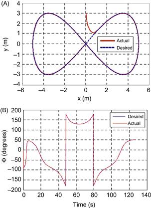
Figure 13.37 (A) Comparison of desired and actual ![]() trajectory achieved by the neurocontroller. (B) Comparison of desired and actual orientation
trajectory achieved by the neurocontroller. (B) Comparison of desired and actual orientation ![]() . Source: Courtesy of J. Velagic [25].
. Source: Courtesy of J. Velagic [25].
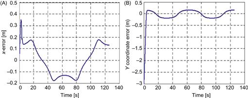
Figure 13.38 Coordinated errors: (A) ![]() error; (B)
error; (B) ![]() error. Source: Courtesy of J. Velagic [25].
error. Source: Courtesy of J. Velagic [25].

Figure 13.39 Linear velocities of the two wheels: (A) left wheel; (B) right wheel. Source: Courtesy of J. Velagic [25].
13.14.2 Navigation for Obstacle Avoidance
The neural nets can be used and have been used for WMR navigation purposes, besides the control purposes. The results to be provided here were obtained by combining MLPs for local modeling of the WMR, and RBFs for the activation of the local models. The division of the input space to subregions was performed using the fuzzy C-means method. For full comprehension of the present mobile robot navigation method, we first describe briefly the concepts of local model NNs (LMNs) and the fuzzy C-means segmentation (FCM) algorithm.
13.14.2.1 Local Model Networks
In this approach, the operation regime is divided in subareas, and each one of them is associated to a local neural model that approximates the system behavior within this subarea. The operating regime includes all the operating points where the system is capable of functioning. Usually, linear neural networks are used. To use the LMNs for system modeling, the parameters that must be included in the operating point (OP) must be determined. The structure of LMN modeling is shown in Figure 13.40 [26–28], where ![]() is the serial number of the local model.
is the serial number of the local model.
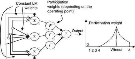
Each linear model is actually a linear predictor, giving a linear estimate of the next value of the system output depending on the previous ones as well as on the past values, namely:
![]()
where ![]() and
and ![]() are the model’s orders with respect to the output
are the model’s orders with respect to the output ![]() and the input
and the input ![]() , respectively. In the special case where
, respectively. In the special case where ![]() , the model reduces to:
, the model reduces to:
![]()
The estimator (predictor) ![]() is trained within each specific part of the operating regime, giving the corresponding coefficients
is trained within each specific part of the operating regime, giving the corresponding coefficients ![]() and
and ![]() . Once there is an LMN trained for every part of the operating regime, the system modeling is complete. The values of its coefficients are given by the estimated values
. Once there is an LMN trained for every part of the operating regime, the system modeling is complete. The values of its coefficients are given by the estimated values ![]() and
and ![]() . In Figure 13.40, the winner-take-all strategy is illustrated, but it is also possible to have a multi-LMN participation for the total system output.
. In Figure 13.40, the winner-take-all strategy is illustrated, but it is also possible to have a multi-LMN participation for the total system output.
13.14.2.2 The Fuzzy C-Means Algorithm
This is an extension of the classical C-means algorithm using fuzzy reasoning, and involves four steps as described below [26,29]. Consider a set of patterns. These are classified (clustered) into c fuzzy clusters by minimizing a cost function of the form:
![]()
• ![]() stands for the membership value of pattern
stands for the membership value of pattern ![]() into cluster
into cluster ![]() ;
;
• ![]() stands for the number of input patterns;
stands for the number of input patterns;
• ![]() stands for the c×N fuzzy partition matrix
stands for the c×N fuzzy partition matrix ![]() ;
;
• ![]() represents the center of ith cluster;
represents the center of ith cluster;
• ![]() stands for the distance between the patterns k and the center of cluster i.
stands for the distance between the patterns k and the center of cluster i.
The steps of the fuzzy C-means algorithm are the following:
Step 1: Define the number c of clusters ![]() , the membership power factor
, the membership power factor ![]() , and the metric used for measuring clusters distance.
, and the metric used for measuring clusters distance.
Step 2: Initialize the fuzzy partition matrix ![]()
(i) Calculate the vectors of the clusters’ centers as ![]()
(ii) Update the fuzzy partition matrix ![]() and find the next one
and find the next one ![]() as follows:
as follows:
Calculate for each pattern ![]() the number of clusters that pattern is associated with:
the number of clusters that pattern is associated with: ![]() , and the set of clusters
, and the set of clusters ![]() to which the pattern is not associated, with the rules:
to which the pattern is not associated, with the rules:
Step 4: Compare ![]() and
and ![]() using the selected measure and if
using the selected measure and if ![]() (convergence threshold), terminate the algorithm; otherwise return to step 3.
(convergence threshold), terminate the algorithm; otherwise return to step 3.
13.14.2.3 Experimental Results
The training process termination criterion of each LMN used is the root mean square (RMS):
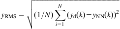
where ![]() is the desired output and
is the desired output and ![]() is the LMN output:
is the LMN output:
![]()
with ![]() being the output estimate of the ith local submodel, and
being the output estimate of the ith local submodel, and ![]() the ith RBF function defined by Eq. (8.62). The results were obtained using 500 learning datasets, each dataset involving five parameters:
the ith RBF function defined by Eq. (8.62). The results were obtained using 500 learning datasets, each dataset involving five parameters:
The experiment used one mobile robot, one target, and four obstacles (if more than one robot exists, each mobile robot is considered as an obstacle to the other robots). The MLP NNs used for local modeling involved three layers (input, hidden, output layer). The input layer has four nodes, that is, three nodes for the input values of the front, left and right distances from obstacles, and one node for the target bearing (if no target is detected, the input to the fourth node is zero). The output layer has a single node which computes the robot steering angle. Figure 13.41A–C shows the path of a single robot followed under the control of an MLP, an RBF, and an LMN (based on MLP and RBF), respectively. Details and statistics of the method are provided in Ref. [26].
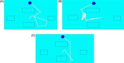
Figure 13.41 Performance of neural network-based navigation: (A) MLP, (B) RBF, and (C) full LMN navigator. Source: Courtesy of H.A. Awad [26].
13.15 Fuzzy Tracking Control of Differential Drive Robot
Here, performance results of the fuzzy logic controller designed by the Mamdani model, as discussed in Section 8.4.1, will be presented. The kinematic model is:
![]()
and the dynamic model in the unconstrained form (3.19a):
![]()
where ![]() ,
, ![]() is the linear friction matrix, and
is the linear friction matrix, and ![]() is an external disturbance, has the parameters [30]:
is an external disturbance, has the parameters [30]:
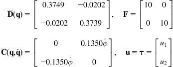
The disturbance vector ![]() is:
is:
![]()
where the delta function ![]() is applied every 2 s. The desired velocity vector
is applied every 2 s. The desired velocity vector ![]() is assumed to be:
is assumed to be:
![]()
and the initial conditions are:
![]()
The crisp kinematic controller used is (see Eq. (8.18)):
![]()
with gains ![]() . The membership functions of the linguistic (fuzzy) variables
. The membership functions of the linguistic (fuzzy) variables ![]() , where
, where ![]() , have the triangular and trapezoidal forms shown in Figure 8.15. The dynamic fuzzy controller has the rule base of Table 8.2 which represents
, have the triangular and trapezoidal forms shown in Figure 8.15. The dynamic fuzzy controller has the rule base of Table 8.2 which represents ![]() fuzzy rules as described in Section 8.4.1. The fuzzy values of
fuzzy rules as described in Section 8.4.1. The fuzzy values of ![]() and
and ![]() are converted to crisp values with the COG defuzzification method and are represented by the input–output surfaces shown in Figure 13.42.
are converted to crisp values with the COG defuzzification method and are represented by the input–output surfaces shown in Figure 13.42.
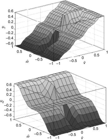
Figure 13.42 Overall input–output surfaces of the fuzzy controller ![]() . Source: Courtesy of O. Castillo [30].
. Source: Courtesy of O. Castillo [30].
The performance of the full controller was tested by simulation on the Matlab (Simulink) in Ref. [30]. It was verified that the error ![]() goes to zero at
goes to zero at ![]() goes to zero at
goes to zero at ![]() , and
, and ![]() goes to zero at
goes to zero at ![]() . The velocity errors were brought to zero at
. The velocity errors were brought to zero at ![]() . The switching behavior of the controller was very fast. The simulation plots of the unperturbed closed-loop control system are shown in Figure 13.43.
. The switching behavior of the controller was very fast. The simulation plots of the unperturbed closed-loop control system are shown in Figure 13.43.
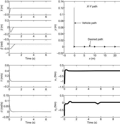
Figure 13.43 Closed-loop performance of the fuzzy controller when ![]() . (A) Errors
. (A) Errors ![]() , and
, and ![]() . (B) xy path and control input (torques)
. (B) xy path and control input (torques) ![]() and
and ![]() . Source: Courtesy of O. Castillo [30].
. Source: Courtesy of O. Castillo [30].
The simulation results for the perturbed system showed again a very good robustness of the controller. Both position and orientation errors converged quickly to zero despite the external disturbances.
13.16 Vision-Based Adaptive Robust Tracking Control of Differential Drive Robot
Here, some results obtained by simulation in Refs. [31,32], using the adaptive robust trajectory tracking controller (9.158a)–(9.158e), will be presented. The system and controller parameters used are given in Table 13.5.
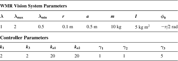
The robot initial pose was ![]() and the desired trajectory started from
and the desired trajectory started from ![]() . The components
. The components ![]() and
and ![]() of
of ![]() were random in the interval
were random in the interval ![]() and
and ![]() . The values of
. The values of ![]() and
and ![]() were selected as
were selected as ![]() and
and ![]() . Figure 13.44 shows the convergence of the errors
. Figure 13.44 shows the convergence of the errors ![]() , and
, and ![]() to zero, despite the existence of the external disturbance.
to zero, despite the existence of the external disturbance.
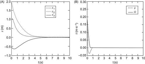
Figure 13.44 (A) Convergence of the errors ![]() , and
, and ![]() . (B) Convergence of the velocity errors. Source: Reprinted from Ref. [31], with permission from Springer Science+Business Media BV.
. (B) Convergence of the velocity errors. Source: Reprinted from Ref. [31], with permission from Springer Science+Business Media BV.
Figure 13.45A shows the torques ![]() which, due to the chattering effect, converge to a small area around zero. Figure 13.45B shows the robot desired and actual trajectory in the world coordinate frame.
which, due to the chattering effect, converge to a small area around zero. Figure 13.45B shows the robot desired and actual trajectory in the world coordinate frame.
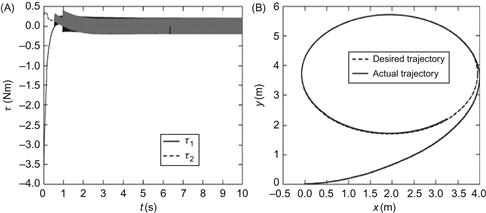
Figure 13.45 (A) The controls ![]() and
and ![]() suffer from chattering. (B) Actual and desired trajectories. Source: Reprinted from Ref. [31], with permission from Springer Science+Business Media BV.
suffer from chattering. (B) Actual and desired trajectories. Source: Reprinted from Ref. [31], with permission from Springer Science+Business Media BV.
The experiments were repeated with the saturation-type controller using a boundary layer width ![]() . Now, the convergence of the errors and the actual trajectory are about the same as in Figures 13.44A and B and 13.45B, but the chattering in the control signals
. Now, the convergence of the errors and the actual trajectory are about the same as in Figures 13.44A and B and 13.45B, but the chattering in the control signals ![]() and
and ![]() disappeared as shown in Figure 13.46.
disappeared as shown in Figure 13.46.
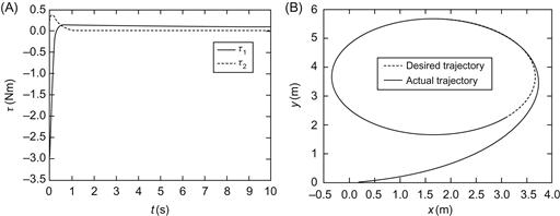
Figure 13.46 (A) Time evolution of ![]() and
and ![]() in the case of saturation-type robustifying control term. (B) Resulting actual trajectory versus desired trajectory. Source: Reprinted from Ref. [31], with permission from Springer Science+Business Media BV.
in the case of saturation-type robustifying control term. (B) Resulting actual trajectory versus desired trajectory. Source: Reprinted from Ref. [31], with permission from Springer Science+Business Media BV.
The estimates of the parameters ![]() and
and ![]() converged to constant values
converged to constant values ![]() , and
, and ![]() . For comparison, the reader is advised to perform a simulation experiment using the alternative controller (9.160) with the same WMR vision system values, desired trajectory, and
. For comparison, the reader is advised to perform a simulation experiment using the alternative controller (9.160) with the same WMR vision system values, desired trajectory, and ![]() values.
values.
13.17 Mobile Manipulator Spherical Catadioptric Visual Control
The problem discussed in Example 10.4 was thoroughly studied in Ref. [33]. The resolved-rate visual servo controller (10.83) was applied using an estimate ![]() of the image Jacobian computed using the EKF technique. Since the parameters involved in the vector
of the image Jacobian computed using the EKF technique. Since the parameters involved in the vector ![]() are constant, the state transition model has the linear form:
are constant, the state transition model has the linear form:
![]() (13.6)
(13.6)
where ![]() is a Gaussian zero-mean disturbance process with covariance matrix
is a Gaussian zero-mean disturbance process with covariance matrix ![]() . The measurement vector is:
. The measurement vector is:
![]()
and the measurement equation is
![]()
where:
![]()
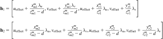
with ![]() a zero-mean Gaussian measurement noise with covariance matrix
a zero-mean Gaussian measurement noise with covariance matrix ![]() . Defining the vector:
. Defining the vector:
![]()
and the ![]() dimensional state vector:
dimensional state vector:
![]()
the measurement equation can take the linear form:
![]() (13.7)
(13.7)
with:
![]()
where, under the assumption that all the components of the state vector ![]() are measurable:
are measurable:
![]()
In the following, a small representative set of simulation results are provided with the following data [33,34]:
• Robot base location in the camera frame: ![]()
• Mirror frame location (with origin at sphere’s center) in the camera frame: ![]()
• Camera intrinsic parameters: ![]()
• Landmarks’ midpoint in robot frame: ![]()
• Landmarks’ connecting line initial orientations: ![]()
• Desired landmarks’ midpoint in robot frame: ![]()
• Landmarks’ connecting line desired orientations: ![]()
• Deviation of camera intrinsic and extrinsic parameters from their real values: average ![]()
Figure 13.47A–D shows a set of results.
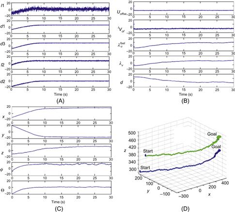
Figure 13.47 (A) Time evolution of the image features’ errors. (B) Camera parameters’ estimates. (C) Midpoint frame pose. (D) 3D trajectories of the landmarks. Source: Reprinted from Ref. [34], with permission from International Society for Optical Engineering (SPIE).
These results verify the decay over time of the features’ errors, the accuracy of the EKF estimates of the camera parameters and image features, and show the actual trajectories of the landmarks in the 3D workspace.
References
1. Gholipour A, Yazdanpanah MJ. Dynamic tracking control of nonholonomic mobile robot with model reference adaptation for uncertain parameters. In: Proceedings of 2003 European control conference (ECC’2003), Cambridge, UK; September 1–4, 2003.
2. Pourboghrat F, Karlsson MP. Adaptive control of dynamic mobile robots with nonholonomic constraints. Comput Electr Eng. 2002;28:241–253.
3. Zhang Y, Hong D, Chung JA, Velinky SA. Dynamic model based robust tracking control of a differentially steered wheeled mobile robot. In: Proceedings of American control conference. Philadelphia, PA; June 1988. p. 850–55.
4. Aicardi M, Casalino G, Bicchi A, Balestrino A. Closed-loop steering of unicycle vehicles via Lyapunov techniques. In: IEEE robotics and automation magazine. March 1995. p. 27–33.
5. Devon D, Bretl T. Kinematic and dynamic control of a wheeled mobile robot. In: Proceedings of 2007 IEEE/RSJ international conference on intelligent robots and systems. San Diego, CA; October 29–November 2, 2007. p. 4065–70.
6. Watanabe K, Yamamoto T, Izumi K, Maeyama S. Underactuated control for nonholonomic mobile robots by using double integrator model and invariant manifold theory. In: Proceedings of 2010 IEEE/RSJ international conference on intelligent robots and systems. Taipei, Taiwan; October 18–22, 2010. p. 2862–67.
7. Rigatos GG, Tzafestas CS, Tzafestas SG. Mobile robot motion control in partially unknown environments using a sliding-mode fuzzy-logic controller. Rob Auton Syst. 2000;33:1–11.
8. Rigatos GG, Tzafestas SG, Evangelidis GJ. Reactive parking control of nonholonomic vehicles via a fuzzy learning automaton. IEE Proc Control Theory Appl. 2001;148(2):169–179.
9. Carelli R, Soria CM, Morales B. Vision-based tracking control for mobile robots. In: Proceedings of twelfth international conference on advanced robotics (ICAR’05). Seatle, WA; July 18–20, 2005. p. 148–52.
10. Gilioli M, Melchiori C. Coordinated mobile manipulator point-stabilization using visual-servoing techniques. In: Proceedings of IEEE/RSJ international conference on intelligent robots and systems (IROS’2002). vol. 1. Lausanne, CH; 2002. p. 305–10.
11. Tsakiris D, Rives P, Samson C. Extending visual servoing techniques to nonholonomic mobile robots. In: Hager G, Kriegman D, Morse S, eds. Vision and control (LNCIS). Berlin: Springer; 1998.
12. Okamoto Jr J, Grassi Jr V. Visual servo control of a mobile robot using omnidirectional vision. In: Van Amerongen J, Jonker B, Regtien P, Stramigiolis S, eds. Proceedings of mechatronics conference 2002. University of Twente June 24–26, 2002;413–422.
13. Abdelkader HH, Mezouar Y, Andreff N, Martinet P. Image-based control of mobile robot with central catadioptric cameras. In: Proceedings of 2005 IEEE international conference on robotics and automation (ICRA 2005). Barcelona, Spain; April 2005. p. 3533–38.
14. Mezouar Y, Abdelkader HH, Martinet P, Chaumette F. Central catadioptric visual servoing from 3D straight lines. In: Proceedings of IEEE/RS international conference on intelligent robots and systems (IROS’04). Sendai, Japan; 2004. p. 343–49.
15. Tzafestas SG, Melfi A, Krikochoritis T. Kinematic/dynamic modeling and control of an omnidirectional mobile manipulator. In: Proceedings of fourth IEEE/IFIP international conference on information technology for balanced automation systems in production and transportation (BASYS2000). Berlin, Germany; 2000.
16. Papadopoulos E, Poulakakis J. Trajectory planning and control for mobile manipulator systems. In: Proceedings of eighth IEEE Mediterranean conference on control and automation (MED’00). Patras, Greece; July 17–19, 2000.
17. Yamamoto Y, Yun X. Coordinating locomotion and manipulation of a mobile manipulator. In: Proceedings of thirty-first IEEE conference on decision and control. Tucson, AZ; 1992. p. 2643–48.
18. Yamamoto Y, Yun X. Modeling and compensation of the dynamic interaction of a mobile manipulator. In: Proceedings of IEEE conference on robotics and automation. San Diego, CA; 1994. p. 2187–92.
19. Zavlangas PG, Tzafestas SG, Althoefer K. Navigation for robotic manipulators employing fuzzy logic. In: Proceedings of third world conference on integrated design and process technology (IDPT’98). vol. 6. Berlin, Germany; 1998. p. 278–83.
20. Zavlagas PG, Tzafestas SG. Integrated fuzzy global path planning and obstacle avoidance for mobile robots. In: Proceedings of European workshop on service and humanoid robots (SERVICEROB’2001). Santorini, Greece; 2001.
21. Tzafestas SG, Stamou G. A fuzzy path planning algorithm for autonomous robots moving in an unknown and uncertain environment. In: Proceedings of European robotics and intelligent systems conference (EURISCON’94). Malaga, Spain; August 1994. p. 140–49.
22. Vidal Calleja TA. Visual navigation in unknown environments. PhD thesis. Barcelona: IRI, The Universitat Politècnica de Catalunya; 2007.
23. Rekleitis I, Dudek G, Milios E. Multirobot collaboration for robust exploration. Ann Math Artif Intell. 2001;31(1–4):7–40.
24. Rekleitis I, Dudek G, Milios E. Probabilistic cooperative localization and mapping in practice. In: Proceedings of IEEE international conference on robotics and automation. vol. 2. Taipei, Taiwan; 2003. p. 1907–12.
25. Velagic J, Osmic N, Lacevic B. Neural network controller for mobile robot motion control. World Acad Sci Eng. 2008;23:193–198.
26. Awad HA, Al-zorkany M. Mobile robot navigation using local model network. Trans Eng Comput Technol. 2004;VI:326–331.
27. Skoundrianos EN, Tzafestas SG. Fault diagnosis via local neural networks. Math Comput Simul. 2002;60:169–180.
28. Skoundrianos EN, Tzafestas SG. Finding fault: diagnosis on the wheels of a mobile robot using local model neural networks. IEEE Rob Autom Mag. 2004;11(3):83–90.
29. Tzafestas SG, Raptis S. Fuzzy image processing: a review and comparison of methods. Image Process Commun. 1999;5(1):3–24.
30. Castillo O, Aguilar LT, Cardenas S. Fuzzy logic tracking control for unicycle mobile robots. Eng Lett. 2006;13(2):73–77 [EL.13-2-4].
31. Yang F, Wang C. Adaptive tracking control for uncertain dynamic nonholonomic mobile robots based on visual servoing. J Control Theory Appl. 2012;10(1):56–63.
32. Wang C, Liang Z, Du J, Liang S. Robust stabilization of nonholonomic moving robots with uncalibrated visual parameters. In: Proceedings of 2009 American control conference. Hyatt Regency River Front, St. Louis, MO; 2009. p.1347–51.
33. Zhang Y. Visual servoing of a 5-DOF mobile manipulator using panoramic vision system. M.A.Sc. thesis. Regina, Canada: Faculty of Engineering, University of Regina; 2007.
34. Zhang Y, Mehrandezh M. Visual servoing of a 5-DOF mobile manipulator using a catadioptric vision system. Proc SPIE Conf Optomechatronic Syst Control III. 2007;6719:6–17.
1In the Takagi–Sugeno method, the rules have the form IF ![]() is
is ![]() AND … AND
AND … AND ![]() , THEN
, THEN ![]() where
where ![]() are crisp-valued coefficients. The total conclusion of this fuzzy system is
are crisp-valued coefficients. The total conclusion of this fuzzy system is ![]() , where
, where ![]() are the weights of the averaging process.
are the weights of the averaging process.