
Mobile Robot Localization and Mapping
Localization and mapping are two of the basic operations needed for the navigation of a robot, the other operations being path planning and motion planning studied in Chapter 11. Other fundamental capabilities and functions of an integrated mobile robotic system, from the task/mission specification to the motion/task execution, are cognition of the task specification, perception of the environment, and control of the robot motion. This chapter is devoted to the localization and map building operations.
Specifically, the objectives of the chapter are (i) to provide the background concepts on stochastic processes, Kalman estimation, and Bayesian estimation employed in WMR localization, (ii) to discuss the sensor imperfections that have to be taken care in their use, (iii) to introduce the relative localization (dead reckoning) concept and present the kinematic analysis of dead reckoning in WMRs, (iv) to study the absolute localization methods (trilateration, triangulation, map matching), (v) to present the application of Kalman filters for mobile robot localization, sensor calibration, and sensor fusion, and (vi) to treat the simultaneous localization and mapping problem via the extended Kalman filter, Bayesian estimation, and particle filter.
Keywords
Mobile robot localization; mobile robot mapping; Kalman filter; extended Kalman filter; Bayesian learning; state prediction; least-squares estimator; sensor imperfections; relative localization; dead reckoning; absolute localization; localization by map matching; resampling; Kalman filter-based localization; Kalman filter-based sensor fusion; simultaneous localization and mapping; Bayesian estimator SLAM; particle filter SLAM
12.1 Introduction
As described in Section 11.3.1, localization and mapping are two of the three basic operations needed for the navigation of a robot. Very broadly, other fundamental capabilities and functions of an integrated robotic system from the task/mission specification to the motion control/task execution (besides path planning) are the following:
A pictorial illustration of the interrelations and organization of the above functions in a working wheel-driven mobile robot (WMR) is shown in Figure 12.1.

The robot must have the ability to perceive the environment via its sensors in order to create the proper data for finding its location (localization) and determining how it should go to its destination in the produced map (path planning). The desired destination is found by the robot through processing of the desired task/mission command with the help of the cognition process. The path is then provided as input to the robot’s motion controller which drives the actuators such that the robot follows the commanded path. The path planning operation was discussed in Chapter 11. Here we will deal with the localization and map building operations. Specifically, the objectives of this chapter are as follows:
• To provide the background concepts on stochastic processes, Kalman estimation, and Bayesian estimation employed in WMR localization
• To discuss the sensor imperfections that have to be taken care in their use
• To introduce the relative localization (dead reckoning) concept, and present the kinematic analysis of dead reckoning in WMRs
• To study the absolute localization methods (trilateration, triangulation, map matching)
• To present the application of Kalman filters for mobile robot localization, sensor calibration, and sensor fusion
• To treat the simultaneous localization and mapping (SLAM) problem via the extended Kalman filter (EKF), Bayesian estimation, and particle filter (PF)
12.2 Background Concepts
Stochastic modeling, Kalman filtering, and Bayesian estimation techniques are important tools for robot localization. Here, an introduction to the above concepts and techniques, which will be used in the chapter, is provided [1–3].
12.2.1 Stochastic Processes
Stochastic process is defined to be a collection (or ensemble) of time functions ![]() of random variables corresponding to an infinitely countable set of experiments
of random variables corresponding to an infinitely countable set of experiments ![]() , with an associated probability description, for example,
, with an associated probability description, for example, ![]() (see Figure 12.2). At time
(see Figure 12.2). At time ![]() ,
, ![]() is a random variable with probability
is a random variable with probability ![]() . Similarly,
. Similarly, ![]() is a random variable with probability
is a random variable with probability ![]() . Here,
. Here, ![]() is a random variable over the ensemble every time, and so we can define first and higher-order statistics for the variables
is a random variable over the ensemble every time, and so we can define first and higher-order statistics for the variables ![]() .
.

First-order statistics is concerned only with a single random variable ![]() and is expressed by a probability distribution
and is expressed by a probability distribution ![]() and its density
and its density ![]() for the continuous-time case, or its distribution function
for the continuous-time case, or its distribution function ![]() for the discrete-time case.
for the discrete-time case.
Second-order statistics is concerned with two random variables ![]() and
and ![]() at two distinct time instances
at two distinct time instances ![]() and
and ![]() . In the continuous-time case, we have the following probability functions for
. In the continuous-time case, we have the following probability functions for ![]() and
and ![]() .
.
![]()
![]()
![]()
![]()
Using the above probability functions we get the first- and second-order averages (moments) as follows:
![]()
![]()
![]()
![]()
The sample statistics time averages of order ![]() over the sample functions of the continuous-time process
over the sample functions of the continuous-time process ![]() are defined as:
are defined as:
![]()
and the time averages of the discrete-time process ![]() as:
as:
![]()
Stationarity: A stochastic process is said to be stationary if all its marginal and joint density functions do not depend on the choice of the time origin. If this is not so, then the process is called nonstationary.
Ergodicity: A stochastic process is said to be ergodic if its ensemble moments (averages) are equal to its corresponding sample moments, that is, if:
![]()
Ergodic stochastic processes are always stationary. The converse does not always hold.
Stationarity and Ergodicity in the Wide Sense: Motivated by the normal (Gaussian) density, which is completely described by its mean and variance, in practice we usually employ only first- and second-order moments. If a process is stationary or ergodic up to second-order moments, then it is called a stationary or ergodic process in the wide sense.
Markov Process: A Markov process is the process in which for ![]() the following property (called Markovian property) is true:
the following property (called Markovian property) is true:
![]() (12.1)
(12.1)
This means that the p.d.f. of the state variable ![]() at some time instant
at some time instant ![]() depends only on the state
depends only on the state ![]() at the immediately previous time
at the immediately previous time ![]() (not on more previous times).
(not on more previous times).
12.2.2 Stochastic Dynamic Models
We consider an n-dimensional linear discrete-time dynamic process described by:
![]() (12.2a)
(12.2a)
![]() (12.2b)
(12.2b)
where ![]() ,
, ![]() ,
, ![]() are matrices of proper dimensionality depending on the discrete-time index
are matrices of proper dimensionality depending on the discrete-time index ![]() , and
, and ![]() ,
, ![]() are stochastic processes (the input disturbance and measurement noise, respectively) with properties:
are stochastic processes (the input disturbance and measurement noise, respectively) with properties:
 (12.3)
where ![]() is the Kronecker delta defined as
is the Kronecker delta defined as ![]() ,
, ![]()
![]() .
.
The initial state ![]() is a random (stochastic) variable, such that:
is a random (stochastic) variable, such that:
![]() (12.4)
(12.4)
The above properties imply that the processes ![]() and
and ![]() and the random variable
and the random variable ![]() are statistically independent. If they are also Gaussian distributed, then the model is said to be a discrete-time Gauss–Markov model (or Gauss–Markov chain), since as can be easily seen, the process
are statistically independent. If they are also Gaussian distributed, then the model is said to be a discrete-time Gauss–Markov model (or Gauss–Markov chain), since as can be easily seen, the process ![]() is Markovian. The continuous-time counterpart of the Gauss–Markov model has an analogous differential equation representation.
is Markovian. The continuous-time counterpart of the Gauss–Markov model has an analogous differential equation representation.
12.2.3 Discrete-Time Kalman Filter and Predictor
We consider a discrete-time Gauss–Markov system of the type described by Eqs. (12.2)–(12.4), with available measurements ![]() . Let
. Let ![]() and
and ![]() be the estimate of
be the estimate of ![]() with measurements up to
with measurements up to ![]() and
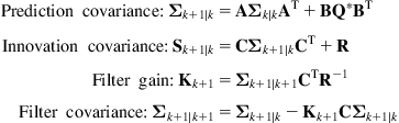
and ![]() , respectively. Then, the discrete-time Kalman filter for the stochastic system (12.2a) with measurement process (12.2b) is described by the following recursive equations:
, respectively. Then, the discrete-time Kalman filter for the stochastic system (12.2a) with measurement process (12.2b) is described by the following recursive equations:
![]() (12.5)
(12.5)
![]() (12.6)
(12.6)
![]() (12.7)
(12.7)
![]() (12.8)
(12.8)
where ![]() is the covariance matrix of the estimate
is the covariance matrix of the estimate ![]() on the basis of data up to time i:
on the basis of data up to time i:
![]() (12.9a)
(12.9a)
![]() (12.9b)
(12.9b)
and the notation ![]() ,
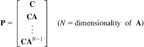
, ![]() , etc. is used. These equations can be represented in the block diagram (Figure 12.3).
, etc. is used. These equations can be represented in the block diagram (Figure 12.3).

Figure 12.3 Block diagram representation of the Kalman filter and predictor (![]() =unit matrix,
=unit matrix, ![]() is the delay operator
is the delay operator ![]() ).
).
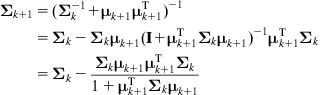
An alternative expression of ![]() is obtained by applying the matrix inversion Lemma, and is the following:
is obtained by applying the matrix inversion Lemma, and is the following:
![]() (12.10)
(12.10)
The initial conditions for the state estimate Eq. (12.5) and the covariance equation (12.7) are:
![]() (12.11)
(12.11)
State Prediction: Using the filtered estimate ![]() of
of ![]() at the discrete-time instant
at the discrete-time instant ![]() , we can compute a predicted estimate
, we can compute a predicted estimate ![]() ,
, ![]() ,
, ![]() of the state
of the state ![]() on the basis of measurements up to the instant
on the basis of measurements up to the instant ![]() . This is done by using the equations:
. This is done by using the equations:
![]() (12.12a)
(12.12a)
![]() (12.12b)
(12.12b)
![]() (12.12c)
(12.12c)
and so on. Therefore:
![]() (12.13)
(12.13)
12.2.4 Bayesian Learning
Formally, the probability of event A occurring, given that the event B occurs, is given by:
![]()
and similarly:
![]()
For notational simplicity, the above formulas are written as:
![]() (12.14)
(12.14)
where ![]() is the probability of
is the probability of ![]() and
and ![]() occurring jointly.
occurring jointly.
Combining the two formulas (12.14), we get the so-called Bayes formula:
![]() (12.15a)
(12.15a)
Now, if ![]() where
where ![]() is a hypothesis (about the truth or cause), and
is a hypothesis (about the truth or cause), and ![]() where
where ![]() represents observed symptoms or measured data or evidence, Eq. (12.15a) gives the so-called Bayes updating (or learning) rule:
represents observed symptoms or measured data or evidence, Eq. (12.15a) gives the so-called Bayes updating (or learning) rule:
![]() (12.15b)
(12.15b)
where ![]() . Here,
. Here, ![]() is the “prior” probability of the hypothesis
is the “prior” probability of the hypothesis ![]() (before any evidence is obtained),
(before any evidence is obtained), ![]() is the probability of the evidence, and
is the probability of the evidence, and ![]() is the probability that the evidence is true when
is the probability that the evidence is true when ![]() holds. The term
holds. The term ![]() is the “posterior” probability (i.e., the “updated” probability) of
is the “posterior” probability (i.e., the “updated” probability) of ![]() after the evidence is obtained. Consider now the case that two evidences
after the evidence is obtained. Consider now the case that two evidences ![]() and
and ![]() about
about ![]() are observed one after the other. Then, Eq. (12.15b) gives:
are observed one after the other. Then, Eq. (12.15b) gives:

Clearly, the above equation says that ![]() , that is, the order in which the evidence (data) are observed does not influence the resulting posterior probability of
, that is, the order in which the evidence (data) are observed does not influence the resulting posterior probability of ![]() given
given ![]() and
and ![]() .
.
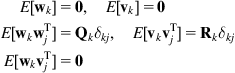
Example 12.1
It is desired to derive the Kalman filter using the least-squares estimation approach.
Solution
The Kalman filter described by Eqs.(12.5)–(12.11) can be derived using several approaches, viz., (i) orthogonality principle, (ii) Gaussian Bayesian technique, and (iii) the least-squares approach (various formulations). Here, the least-squares estimator (3.103) will be used which was derived for the measurement system (3.102). This estimator uses all available data ![]() at once, and provides an off-line estimate of
at once, and provides an off-line estimate of ![]() . The derivation of the Kalman filter (12.5)–(12.11) will be done by converting Eq. (3.103) to recursive form that updates (improves) the estimate
. The derivation of the Kalman filter (12.5)–(12.11) will be done by converting Eq. (3.103) to recursive form that updates (improves) the estimate ![]() (found on the basis of
(found on the basis of ![]() measurements
measurements ![]() ) using the next,
) using the next, ![]() , measurement
, measurement ![]() . To this end, we define:
. To this end, we define:
 (12.16a)
The matrices ![]() and
and ![]() are related as follows:
are related as follows:

Therefore:
![]() (12.16b)
(12.16b)
Now, using Eqs. (3.103) and (12.16a) we get:
![]()
![]()
To express ![]() in terms of
in terms of ![]() we must eliminate
we must eliminate ![]() from the above equations. The first of these equations gives
from the above equations. The first of these equations gives ![]() . Thus, the second equation can be written as:
. Thus, the second equation can be written as:
 (12.17a)
Equation (12.17a) provides the desired recursive least-squares estimator. The new estimate ![]() is a function of the old estimate
is a function of the old estimate ![]() , the new data pair
, the new data pair ![]() and the matrix
and the matrix ![]() . Actually, the new estimate
. Actually, the new estimate ![]() is equal to the old estimate
is equal to the old estimate ![]() plus a correction term equal to an adaptation (or learning) gain vector
plus a correction term equal to an adaptation (or learning) gain vector ![]() multiplied by the prediction (learning) error or innovation process
multiplied by the prediction (learning) error or innovation process ![]() . For this reason Eq. (12.17a) is also called “least-squares learning equation or rule.” We now have to find how
. For this reason Eq. (12.17a) is also called “least-squares learning equation or rule.” We now have to find how ![]() can be found from
can be found from ![]() .
.
From Eq. (12.16b) we obtain:1
 (12.17b)
for ![]() (since
(since ![]() is a scalar). The full recursive least-squares estimation algorithm given by Eqs. (12.17a) and (12.17b) is initiated using selected initial values
is a scalar). The full recursive least-squares estimation algorithm given by Eqs. (12.17a) and (12.17b) is initiated using selected initial values ![]() and
and ![]() . One may also start from
. One may also start from ![]() , by using the first
, by using the first ![]() measurements to get
measurements to get ![]() and
and ![]() directly:
directly:
![]()
Now, using in Eqs. (12.17a) and (12.17b) the following variable substitutions:
![]()
we get the Kalman filter Eqs. (12.5)–(12.11).
The initial conditions for the state estimate Eq. (12.5) and the covariance equation (12.7) are:
![]()
To see how the Kalman filter works, we consider a scalar time-invariant discrete-time Gauss–Markov system:
![]()
with ![]() ,
, ![]() ,
, ![]() , and
, and ![]() . The Kalman filter Eqs. (12.5)–(12.11) give:
. The Kalman filter Eqs. (12.5)–(12.11) give:
![]()
![]()
![]()
![]()
Since ![]() , the second equation tells us that
, the second equation tells us that ![]() , that is, the one-step prediction accuracy is at minimum equal to the variance of the input disturbance
, that is, the one-step prediction accuracy is at minimum equal to the variance of the input disturbance ![]() . From the third equation, we see that
. From the third equation, we see that ![]() . The fourth equation implies that
. The fourth equation implies that ![]() . Thus,
. Thus, ![]() . This means that if
. This means that if ![]() , the use of the first measurement
, the use of the first measurement ![]() gives
gives ![]() , that is, it provides a drastic reduction in the estimation error. Using the given values
, that is, it provides a drastic reduction in the estimation error. Using the given values ![]() ,
, ![]() ,
, ![]() , and
, and ![]() , the variance equations give the results as shown in Table 12.1.
, the variance equations give the results as shown in Table 12.1.
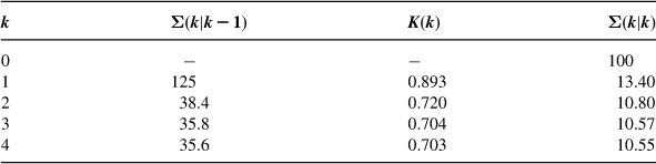
The steady-state value of ![]() is found by setting
is found by setting ![]() , in which case we obtain
, in which case we obtain ![]() . Since
. Since ![]() , the acceptable solution is
, the acceptable solution is ![]() . Thus,
. Thus, ![]() , and
, and
![]()
1Using the following matrix inversion lemma: ![]() with
with ![]() ,
, ![]() , and
, and ![]() .
.
12.3 Sensor Imperfections
The primary prerequisite for an accurate localization is the availability of reliable high-resolution sensors. Unfortunately, the practically available real-life sensors have several imperfections that are due to different causes. As we saw in Chapter 4, the usual sensors employed in robot navigation are range finders via sonar, laser and infrared technology, radar, tactile sensors, compasses, and GPS. Sonars have very low spatial bandwidth capabilities and are subject to noise due to wave scattering, and so the use of laser range sensing is preferred. But despite laser sensors possess a much wider bandwidth, they are still affected by noise. Furthermore, lasers have a restricted field of view, unless special measures are taken (e.g., incorporation of rotating mirrors in the design).
Since both sonar-based and laser-based navigation have the above drawbacks, robotic scientists have strengthened their attention to vision sensors and camera-based systems. Vision sensors can offer a wide field of view, millisecond sampling rates, and are easily applicable for control purposes. Some of the drawbacks of vision are the lack of depth information, image occlusion, low resolution, and the need for recognition and interpretation. However, despite the relative advantages and disadvantages, the use of monocular cameras as a sensor for navigation leads to a competitive selection.
In general, the sensor imperfections can be grouped in: sensor noise and sensor aliasing categories [4–8]. The sensor noise is primarily caused by the environmental variations that cannot be captured by the robot. Examples of this in vision systems are the illumination conditions, the blooming, and the blurring. In sonar systems, if the surface accepting the emitted sound is relatively smooth and angled, much of the signal will be reflected away, failing to produce a return echo. Another source of noise in sonar systems is the use of multiple sonar emitters (16–40 emitters) that are subject to echo interference effects. The second imperfection of robotic sensors is the aliasing, that is, the fact that sensor readings are not unique. In other words, the mapping from the environmental states to the robot’s perceptual inputs is many-to-one (not one-to-one). The sensor aliasing implies that (even if no noise exists) the available amount of information is in most cases not sufficient to identify the robot’s position from a single sensor reading. The above issues suggest that in practice special sensor signal processing/fusion techniques should be employed to minimize the effect of noise and aliasing, and thus get an accurate estimate of the robot position over time. These techniques include probabilistic and information theory methods (Bayesian estimators, Kalman filters, EKFs, PFs, Monte Carlo estimators, information filters, fuzzy/neural approximators, etc).
12.4 Relative Localization
Relative localization is performed by dead reckoning, that is, by the measurement of the movement of a wheeled mobile robot (WMR) between two locations. This is done repeatedly as the robot moves and the movement measurements are added together to form an estimate of the distance traveled from the starting position. Since the individual estimates of the local positions are not exact, the errors are accumulated and the absolute error in the total movement estimate increases with traveled distance. The term dead reckoning comes from the sailing days term “deduced reckoning” [4].
For a WMR, the dead reckoning method is called “odometry,” and is based on data obtained from incremental wheel encoders [9].
The basic assumption of odometry is that wheel revolutions can be transformed into linear displacements relative to the floor. This assumption is rarely ideally valid because of wheel slippage and other causes. The errors in odometric measurement are distinguished in:
• Systematic errors (e.g., due to unequal wheel diameters, misalignment of wheels, actual wheel base is different than nominal wheel base, finite encoder resolution, encoder sampling rate).
• Non-systematic errors (e.g., uneven floors, slippery floors, overacceleration, nonpoint contact with the floor, skidding/fast turning, internal and external forces).
Systematic errors are cumulative and occur principally in indoor environment. Nonsystematic errors are dominating in outdoor environments.
Two simple models for representing the systematic odometric errors are:
Error due to unequal wheel diameter:
![]()
Error due uncertainty about the effective wheel base:
![]()
where ![]() ,
, ![]() are the actual diameters of the right and left wheels, respectively, and
are the actual diameters of the right and left wheels, respectively, and ![]() is the wheel base. It has been verified that either
is the wheel base. It has been verified that either ![]() or
or ![]() can cause the same final error in both position and orientation measurement. To estimate the nonsystematic errors, we use the worst possible case, that is, we estimate the biggest possible disturbance. A good measure of nonsystematic errors is provided by the average absolute orientation errors
can cause the same final error in both position and orientation measurement. To estimate the nonsystematic errors, we use the worst possible case, that is, we estimate the biggest possible disturbance. A good measure of nonsystematic errors is provided by the average absolute orientation errors ![]() clockwise and counterclockwise directions, namely
clockwise and counterclockwise directions, namely ![]() and
and ![]() , respectively. Some ways for reducing systematic odometry errors are:
, respectively. Some ways for reducing systematic odometry errors are:
• Addition of auxiliary wheels (a pair of “knife-edge,” nonload-bearing encoder wheels; Figure 12.4).

Methods for reducing nonsystematic odometry errors include:
• Mutual referencing (use of two robots that measure their positions mutually).
• Correction internal position error (two WMRs mutually correct their odometry errors).
Clearly, more accurate odometry reduces the requirements on absolute position updates, but does not eliminate completely the necessity for periodic updating of the absolute position.
12.5 Kinematic Analysis of Dead Reckoning
The robot state (position and orientation) at instant ![]() is
is ![]() . The dead-reckoning (odometry)-based localization of WMRs is to estimate
. The dead-reckoning (odometry)-based localization of WMRs is to estimate ![]() at instant
at instant ![]() , and linear and angular position increments
, and linear and angular position increments ![]() , and
, and ![]() , respectively, between the time instants
, respectively, between the time instants ![]() and
and ![]() , where
, where ![]() ,
, ![]() , and
, and ![]() . Assuming that
. Assuming that ![]() is very small, we have the following approximations:
is very small, we have the following approximations:
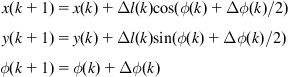
To determine the position and angle increments from the wheel movements (i.e., the encoder values), we must use the kinematic equations of the WMR under consideration. We therefore investigate the localization problem for differential drive, tricycle drive, synchrodrive, Ackerman steering, and omnidirectional drive.
12.5.1 Differential Drive WMR
In this case, two optical encoders are sufficient. They supply the increments ![]() and
and ![]() of the left and right wheels. If
of the left and right wheels. If ![]() is the distance of the two wheels, and
is the distance of the two wheels, and ![]() the instantaneous curvature radius, we have:
the instantaneous curvature radius, we have:
![]()
and therefore:
![]()
Now
 (12.18a)
and
![]() (12.18b)
(12.18b)
These formulas give ![]() and
and ![]() in terms of the encoders’ values
in terms of the encoders’ values ![]() and
and ![]() .
.
12.5.2 Ackerman Steering
We work using the robot’s diagram of Figure 1.28 denoted by ![]() the length of the vehicle (from the rotation axis of the back wheels to the axis of the front axis). We have:
the length of the vehicle (from the rotation axis of the back wheels to the axis of the front axis). We have:
![]()
where ![]() is the actual steering angle of the vehicle (i.e., the angle of the virtual wheel located in the middle of the two front wheels), and
is the actual steering angle of the vehicle (i.e., the angle of the virtual wheel located in the middle of the two front wheels), and ![]() ,
, ![]() are the steering angles of the outer and inner wheel, respectively.
are the steering angles of the outer and inner wheel, respectively.
Working as in the differential drive case, we find:
![]() (12.19a)
(12.19a)
![]() (12.19b)
(12.19b)
Here, we also find:
![]() (12.20)
(12.20)
Two encoders are sufficient to provide ![]() and
and ![]() using the two relations (12.19a) and (12.19b). To use Eq. (12.20) we need a third encoder. But the result can be used to decrease the errors of the other two encoders.
using the two relations (12.19a) and (12.19b). To use Eq. (12.20) we need a third encoder. But the result can be used to decrease the errors of the other two encoders.
12.5.3 Tricycle Drive
Here, the solution is the same as that for the Ackerman steering:
![]() (12.21)
(12.21)
![]() (12.22)
(12.22)
12.6 Absolute Localization
12.6.1 General Issues
Landmarks and beacons form the basis for absolute localization of a WMR [10]. Landmarks may or may not have identities. If the landmarks have identities, no a priori knowledge about the navigating robot’s position is needed. Otherwise, if landmarks have no identities some rough knowledge of the position of the robot must be available. If natural landmarks are employed, then the presence or not of identities depends on the environment. For example, in an office building, one of the rooms may have a large three-glass window, which can be used as a landmark with identity.
The landmarks (beacons) are distinguished in:
An active landmark emits some kind of signal to enable easy detection. In general, the detection of a passive landmark needs more of the sensor. To simplify the detection of passive landmarks, we may use an active sensor together with a passive landmark that responds to this activeness. For example, use of bar codes on walls and visual light to detect them for building topological maps. It is preferable that natural landmarks can be employed with sustainable robustness of the navigational system. They can provide increased flexibility to the adaptation to new environments with minimum requirement of engineering design. For example, natural landmarks in indoor environments can be chairs, desks, and tables.
According to Borenstein [4], localization using active landmarks is distinguished in:
12.6.2 Localization by Trilateration
In trilateration, the location of a WMR is determined using distance measurements to known active beacon, ![]() . Typically, three or more transmitters are used and one receiver on the robot. The locations of transmitters (beacons) must be known. Conversely, the robot may have one transmitter onboard and the receivers can be placed at known positions in the environment (e.g., on the walls of a room). Two examples of localization by trilateration are the beacon systems that use ultrasonic sensors (Figure 12.5) and the GPS system (Figure 4.24b).
. Typically, three or more transmitters are used and one receiver on the robot. The locations of transmitters (beacons) must be known. Conversely, the robot may have one transmitter onboard and the receivers can be placed at known positions in the environment (e.g., on the walls of a room). Two examples of localization by trilateration are the beacon systems that use ultrasonic sensors (Figure 12.5) and the GPS system (Figure 4.24b).
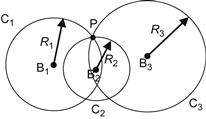
Figure 12.5 Graphical illustration of localization by trilateration. The robot ![]() lies at the intersection of the three circles
lies at the intersection of the three circles ![]() centered at the beacons
centered at the beacons ![]() with radii
with radii ![]()
![]() .
.
Ultrasonic-based trilateration localization systems are appropriate for use in relatively small area environments (because of the short range of ultrasound), where no obstructions that interfere with the wave transmission exist. If the environment is large, the installation of multiple networked beacons throughout the operating area is of increased complexity, a fact that reduces the applicability a sonar-based trilateration. The two alternative designs are:
• Use of a single transducer transmitting from the robot with many receivers at fixed positions.
• Use of a single listening receiver on the robot, with multiple fixed transmitters serving as beacons (this is analogous to the GPS concept).
The position ![]() of the robot in the world coordinate system can be found by least-squares estimation as follows. In Figure 12.5, let
of the robot in the world coordinate system can be found by least-squares estimation as follows. In Figure 12.5, let ![]() be the known world coordinates of the beacons
be the known world coordinates of the beacons ![]() and
and ![]() the corresponding robot–beacon distances (radii of the intersecting circles). Then, we have:
the corresponding robot–beacon distances (radii of the intersecting circles). Then, we have:
![]()
Expanding and rearranging gives:
![]()
To eliminate the squares of the unknown variables ![]() and
and ![]() , we pairwise subtract the above equations, for example, we subtract the kth equation from the ith equation to get:
, we pairwise subtract the above equations, for example, we subtract the kth equation from the ith equation to get:
![]()
where:
![]()
Overall, we obtain the following overdetermined system of linear equations with two unknowns:
![]()

The solution of this linear algebraic system is given by (see Eqs. (2.7) and (2.8a)):
![]()
under the assumption that the matrix ![]() is invertible.
is invertible.
An alternative way of computing ![]() is to apply the general iterative least-squares technique for nonlinear estimation. To this end, we expand the nonlinear function:
is to apply the general iterative least-squares technique for nonlinear estimation. To this end, we expand the nonlinear function:
![]()
in Taylor series about an a priori position estimate ![]() , and keep only first-order terms, namely:
, and keep only first-order terms, namely:
![]()
where:
![]()
and ![]() is the Jacobian matrix of
is the Jacobian matrix of ![]() evaluated at
evaluated at ![]() :
:
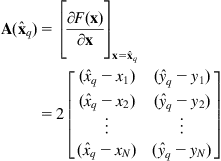
Therefore, we get the following iterative equation for updating the estimate ![]() :
:
![]()
where ![]() is known.
is known.
The iteration is repeated until ![]() becomes smaller than a predetermined small number
becomes smaller than a predetermined small number ![]() or the number of iterations arrives at a maximum number
or the number of iterations arrives at a maximum number ![]() .
.
In practice, due to measurement errors in the positions of the beacons and the radii of the circles, the circles do not intersect at a single point but overlap in a small region. The position of the robot is somewhere in this region. Each pair of circles gives two intersection points, and so with three circles (beacons) we have six intersection points. Three of these points are clustered together more closely than the other three points. A simple procedure for determining the smallest intersection (clustering) region is as follows:
• Compute the distance between each pair of circle intersection points.
• Select the two closest intersection points as the initial cluster.
• Compute the centroid of this cluster (The x,y coordinates of the centroid are obtained by the averages of the x,y coordinates of the points in the cluster).
• Find the circle intersection point which is closest to the cluster centroid.
• Add this intersection point to the cluster and compute again the cluster centroid.
• Continue in the same manner until N intersection points have been added to the cluster, where N is the number of beacons (circles).
• The location of the robot is given by the centroid of the final cluster.
As an exercise, the reader may consider the case of two beacons (circles) and compute geometrically the positions of their intersection points. Also, the conditions under which the solution is nonsingular must be determined.
12.6.3 Localization by Triangulation
In this method, there are three or more active beacons (transmitters) mounted at known positions in the workspace (Figure 12.6). A rotating sensor mounted on the robot ![]() registers the angles
registers the angles ![]() ,
, ![]() , and
, and ![]() at which the robot “sees” the active beacons relative to the WMR’s longitudinal axis
at which the robot “sees” the active beacons relative to the WMR’s longitudinal axis ![]() . Using these three readings, we can compute the position
. Using these three readings, we can compute the position ![]() of the robot, where x stands for X0 and y stands for Y0.
of the robot, where x stands for X0 and y stands for Y0.

Figure 12.6 Triangulation method. A rotating sensor head measures the angles ![]() between the three active beacons
between the three active beacons ![]() ,
, ![]() , and
, and ![]() and the robot’s longitudinal axis.
and the robot’s longitudinal axis.
The active beacons must be sufficiently powerful in order to be able to transmit the appropriate signal power in all directions. The two design alternatives of triangulation are:
It must be noted that when the observed angles are small, or the observation point is very near to a circle containing the beacons, the triangulation results are very sensitive to small angular errors. The three-point triangulation method works efficiently only when the robot lies inside the boundary of the triangle formed by the three beacons. The geometric circle intersection shows large errors when the three beacons and the robot all lie on or are very close to the same circle. In case the Newton–Raphson method is used to determine the robot’s location, no solution can be provided if the initial guess of the robot’s position/orientation is in the exterior of a certain bound. A variation of the triangular method creates a virtual beacon as follows: a range or angle obtained from a beacon at time ![]() can be used at time
can be used at time ![]() , provided that the cumulative movement vector, recorded since the reading was obtained, is added to the position vector of the beacon. This generates a new virtual beacon.
, provided that the cumulative movement vector, recorded since the reading was obtained, is added to the position vector of the beacon. This generates a new virtual beacon.
Referring to Figure 12.6, the basic trigonometric equation, which relates x,y, and ![]() with the measured angles
with the measured angles ![]() of the beacons, is:
of the beacons, is:
![]()
where ![]() are the coordinates of the beacon
are the coordinates of the beacon ![]() . Three beacons are sufficient for computing
. Three beacons are sufficient for computing ![]() under the condition that the measurements are noise free. Then, we will have a nonlinear algebraic system of three equations with three unknowns which can be solved by approximate numerical techniques such as the Newton–Raphson technique and its variations. But if the measurements are noisy (as it typically happens in practice), we need more beacons. In this case, we get an overdetermined noisy nonlinear algebraic system which can be solved by the iterative least-squares technique, in analogy to the above-mentioned trilateration method [11].
under the condition that the measurements are noise free. Then, we will have a nonlinear algebraic system of three equations with three unknowns which can be solved by approximate numerical techniques such as the Newton–Raphson technique and its variations. But if the measurements are noisy (as it typically happens in practice), we need more beacons. In this case, we get an overdetermined noisy nonlinear algebraic system which can be solved by the iterative least-squares technique, in analogy to the above-mentioned trilateration method [11].
The results obtained are more accurate if the artificial beacons are optimally placed (e.g., if they are about ![]() apart in the three-beacon case). Otherwise, the robot position and orientation may have large variations with respect to an optimal value. Moreover, if all beacons are identical, it is very difficult to identify which beacon has been detected. Finally, mismatch is likely to occur if the presence of obstacles in the environment obscures one or more beacons. A natural way to overcome the problem of distinguishing one beacon from another is to manually initialize and recalibrate the robot position when the robot is lost. However, such a manual initialization/recalibration is not convenient in actual applications. Therefore, many automated initialization/recalibration techniques have been developed for use in robot localization by triangulation. One of them uses a self-organizing neural network (Kohonen network) which is able to recognize and distinguish the beacons [12] (see also Section 12.7).
apart in the three-beacon case). Otherwise, the robot position and orientation may have large variations with respect to an optimal value. Moreover, if all beacons are identical, it is very difficult to identify which beacon has been detected. Finally, mismatch is likely to occur if the presence of obstacles in the environment obscures one or more beacons. A natural way to overcome the problem of distinguishing one beacon from another is to manually initialize and recalibrate the robot position when the robot is lost. However, such a manual initialization/recalibration is not convenient in actual applications. Therefore, many automated initialization/recalibration techniques have been developed for use in robot localization by triangulation. One of them uses a self-organizing neural network (Kohonen network) which is able to recognize and distinguish the beacons [12] (see also Section 12.7).
12.6.4 Localization by Map Matching
Map-matching-based localization is a method in which a robot uses its sensors to produce a map of its local environment [13]. When we talk about a map in real life, we usually imagine a geometrical map like the map of a country or a town with names of places and streets. To find our way in a map of a city using street names, we walk up to a street corner, read the name (i.e., the landmark) and compare the name with what is written in the map. Now, if we know where we wish to go, we plan a path to this goal. In our way, we use natural landmarks (e.g., street corners, buildings, streets, blocks) to keep track of where we are along the planned path. If we lose track we have to revert the reading signs and matching the street names to the map. If a road is closed, dead-end, or one-way street, then we plan an alternative path. This methodology is in principle used by WMRs in map generation and matching, of course with landmarks suitable for the robot’s environment in each case.
The robot compares its local map to a global map already stored in the computer’s memory. If a match is found, then the robot can determine its actual position and orientation in the environment. The prestored map may be a CAD model of the environment, or it can be created from prior sensor data.
The basic structure of a map-based localization system is shown in Figure 12.7.
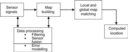
Figure 12.7 Structure of map-based localization (search can be reduced if the initial position guess is close to the true position).
The benefits of the map-based positioning method are the following:
• No modification of the environment is required (only structured natural landmarks are needed).
• Generation of an updated map of the environment can be made.
• The robot can learn a new environment and enhance positioning accuracy via exploration.
Some drawbacks are as follows:
• A sufficient number of stationary, easily distinguishable, features are needed.
• The accuracy of the map must be sufficient for the tasks at hand.
• A substantial amount of sensing and processing power is required.
Maps are distinguished as follows:
Topological maps: They are suitable for sensors that provide information about the identity of landmarks. A real-life topological map example is the subway map which provides information only on how you get from one station (place) to another (no information about distances is given). To enable easy orientation when changing trains, color codings are provided. Topological maps model the world by a network of arcs and nodes.
Geometrical maps: These maps can be constructed from topological maps if the proper equipment for measuring distance and angle is available. Geometrical maps suit sensors that provide geometrical information (e.g., range), like sonar and laser range finders. In general, it is easier to use geometrical maps in conjunction with sensors of this type, than using topological maps, since less advanced perception techniques are needed. In extreme situations, the sensor measurements can be directly matched to the stored map.
Currently, used maps are often CAD drawings or they have been measured by hand. The human is deciding on which parts of the environment should be included in the map. It is also up to the human to decide which sensor is the most appropriate to use (taking of course into account its price), and how it will respond to the environment. Ideally, it is desired that the WMR is able to construct maps autonomously by itself. In this direction, a solid methodology called simultaneous localization and mapping has been developed which will be examined in the following text.
12.7 Kalman Filter-Based Localization and Sensor Calibration and Fusion
The Kalman filter described by Eqs. (12.5)–(12.11) can be used for three purposes, namely:
12.7.1 Robot Localization
The steps of the localization algorithm that is based on Kalman filter are the following:
Step 1—One-Step Prediction
The predicted robot position ![]() at time
at time ![]() , given the known filtered position
, given the known filtered position ![]() at time
at time ![]() , is given by Eq. (12.12a), that is:
, is given by Eq. (12.12a), that is:
![]() (12.24)
(12.24)
where ![]() represents the kinematic equation of the robot. The corresponding position uncertainty is given by the covariance matrix
represents the kinematic equation of the robot. The corresponding position uncertainty is given by the covariance matrix ![]() described by Eq. (12.8), that is:
described by Eq. (12.8), that is:
![]() (12.25)
(12.25)
with ![]() (a known value). The respective prediction
(a known value). The respective prediction ![]() of the sensors’ measurements is given by:
of the sensors’ measurements is given by:
![]()
Step 2—Sensor Observation
At this step, a new set of sensor measurements ![]() at time
at time ![]() is taken.
is taken.
Step 3—Matching
The measurement innovation process:
 (12.26)
![]() (12.27)
(12.27)
is constructed.
Step 4—Position Estimation
Calculate the Kalman filter gain matrix ![]() using Eq. (12.10), that is:
using Eq. (12.10), that is:
![]() (12.28)
(12.28)
and the updated position estimate ![]() is given by Eqs. (12.5)–(12.8), that is:
is given by Eqs. (12.5)–(12.8), that is:
![]() (12.29)
(12.29)
![]() (12.30)
(12.30)
where ![]() and
and ![]() are given by Eqs. (12.26) and (12.25), respectively. The initial value
are given by Eqs. (12.26) and (12.25), respectively. The initial value ![]() of the estimate’s covariance, as well as the values of
of the estimate’s covariance, as well as the values of ![]() and
and ![]() needs to be determined experimentally (before the application of the method) using the available information about the sensors and their models. Typically,
needs to be determined experimentally (before the application of the method) using the available information about the sensors and their models. Typically, ![]() and
and ![]() Taking into account that the measurement (sensor observation) vector
Taking into account that the measurement (sensor observation) vector ![]() may involve data from several sensors (usually of different type), we can say that the Kalman filter provides also a sensor fusion and integration method (see Example 12.5).
may involve data from several sensors (usually of different type), we can say that the Kalman filter provides also a sensor fusion and integration method (see Example 12.5).
In all cases, it is advised to check if the new measurements are statistically independent from the previous measurements and disregard them if they are statistically dependent, since they do not actually provide new information. This can be done at the matching step on the basis of the innovation process (or residual) ![]() and its covariance
and its covariance ![]() given by Eqs. (12.26) and (12.27). The process
given by Eqs. (12.26) and (12.27). The process ![]() expresses the difference between the new measurement
expresses the difference between the new measurement ![]() and its expected value
and its expected value ![]() according to the system model.
according to the system model.
To this end, we use the so-called normalized innovation squared (NIS) defined as:
![]()
The process ![]() follows a chi-square
follows a chi-square ![]() distribution with
distribution with ![]() degrees of freedom (more precisely when the innovation process
degrees of freedom (more precisely when the innovation process ![]() is Gaussian). Therefore, we can read from the chi-square, the bounding values (confidence interval) for a
is Gaussian). Therefore, we can read from the chi-square, the bounding values (confidence interval) for a ![]() random variable with
random variable with ![]() degrees of freedom, and discard a measurement, if its
degrees of freedom, and discard a measurement, if its ![]() is outside the desired confidence interval. More specifically, if the criterion:
is outside the desired confidence interval. More specifically, if the criterion:
![]()
is satisfied, then the measurement ![]() is considered to be independent from
is considered to be independent from ![]() and so it is included in the filtering process. Measurements that do not satisfy the above criterion are ignored. The random variable
and so it is included in the filtering process. Measurements that do not satisfy the above criterion are ignored. The random variable ![]() is defined as follows. Consider two random variables (sensor signals)
is defined as follows. Consider two random variables (sensor signals) ![]() and
and ![]() which are independent if the probability distribution of
which are independent if the probability distribution of ![]() is not affected by the presence of
is not affected by the presence of ![]() . Then, the chi-square variable is given by:
. Then, the chi-square variable is given by:
![]()
where ![]() is the observed frequency of events belonging to both the ith category of
is the observed frequency of events belonging to both the ith category of ![]() and
and ![]() category of
category of ![]() , and
, and ![]() is the corresponding expected frequency of events if
is the corresponding expected frequency of events if ![]() and
and ![]() are independent. The use of chi-square (or contingency table) is described in books on statistics (see, e.g., in http://onlinestatbook.com/stat_sim/chisq_theory/index.html).
are independent. The use of chi-square (or contingency table) is described in books on statistics (see, e.g., in http://onlinestatbook.com/stat_sim/chisq_theory/index.html).
12.7.2 Sensor Calibration
The Kalman filter provides also a method for sensor calibration, which is based on the minimization of the error between the actual measurements and the simulated measurement of the sensor with the parameters at hand. The parameters that have to be calibrated may be intrinsic or extrinsic. Intrinsic parameters cannot be directly observed, but extrinsic parameters can. For instance, the focal distance, the location of the optical center, and the distortion of a camera are intrinsic parameters, but the position of the camera is an extrinsic parameter.
To perform sensor calibration with the aid of the Kalman filter, we use the parameters under calibration, as the state vector of the model, in place of the robot’s position/orientation. The prediction step gives simulated values of the parameters at the present state (i.e., with their present values). The state observation step provides a set of sensor captions taken at different robot positions, and not during the motion of the robot (as we did for robot localization, i.e., for position estimation and mapping). The use of Kalman filters for sensor calibration is general and independent of the nature of the sensor (range, vision, etc.). The only things that change are the state vector ![]() and the measurement vector with the associated matrices
and the measurement vector with the associated matrices ![]() ,
, ![]() , and
, and ![]() , and the noises
, and the noises ![]() and
and ![]() .
.
12.7.3 Sensor Fusion
Sensor fusion is the process of merging data from multiple sensors such that to reduce the amount of uncertainty that may be involved in a robot navigation motion or task performing. Sensor fusion helps in building a more accurate world model in order for the robot to navigate and behave more successfully. The three fundamental ways of combining sensor data are the following:
• Redundant sensors: All sensors give the same information for the world.
• Complementary sensors: The sensors provide independent (disjoint) types of information about the world.
• Coordinated sensors: The sensors collect information about the world sequentially.
The three basic sensor communication schemes are [14]:
• Decentralized: No communication exists between the sensor nodes.
• Centralized: All sensors provide measurements to a central node.
• Distributed: The nodes interchange information at a given communication rate (e.g., every five scans, i.e., one-fifth communication rate).
The centralized scheme can be regarded as a special case of the distributed scheme where the sensors communicate to each other every scan. A pictorial representation of the fusion process is given in Figure 12.8.

Consider, for simplicity, the case of two redundant local sensors (N=2). Each sensor processor ![]() provides its own prior and updated estimates and covariances
provides its own prior and updated estimates and covariances ![]() ,
, ![]() and
and ![]() ,
, ![]() ,
, ![]() . Assume that the fusion processor has its own total prior estimate
. Assume that the fusion processor has its own total prior estimate ![]() and
and ![]() . The fusion problem is to compute the total estimate
. The fusion problem is to compute the total estimate ![]() and covariance matrix
and covariance matrix ![]() using only those local estimates and the total prior estimate. The total updated estimate can be obtained using linear operations on the local estimates, as:
using only those local estimates and the total prior estimate. The total updated estimate can be obtained using linear operations on the local estimates, as:

![]()
When the local processors and the fusion processor have the same prior estimates, the above fusion equations can be simplified as:
 (12.31a)
![]() (12.31b)
(12.31b)
This means that the common prior estimates (i.e., the redundant information) are subtracted in the linear fusion operation. The above equations constitute the fusion processor shown in Figure 12.8. Typically, the sensor processors ![]() are Kalman filters.
are Kalman filters.
Example 12.2
We will derive the formula for fusing the measurements ![]() provided for a quantity
provided for a quantity ![]() (e.g., the position of a WMR) by
(e.g., the position of a WMR) by ![]() independent sensors. It is assumed that the measurement
independent sensors. It is assumed that the measurement ![]() of the kth sensor is normally distributed (Gaussian) with variance
of the kth sensor is normally distributed (Gaussian) with variance ![]() .
.
We will apply the maximum likelihood estimation method in which the joint probability distribution ![]() of
of ![]() is maximized with respect to the fused value
is maximized with respect to the fused value ![]() and fused variance
and fused variance ![]() . The joint Gaussian distribution
. The joint Gaussian distribution ![]() is:
is:
![]()
The likelihood function ![]() is defined as the logarithm of
is defined as the logarithm of ![]() , that is:
, that is:
![]()
To maximize L, we equate to zero the derivative of ![]() with respect to
with respect to ![]() , that is:
, that is:
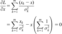
Thus, the fused estimate ![]() of the
of the ![]() sensors is equal to:
sensors is equal to:

The variance ![]() of
of ![]() is given by:
is given by:
![]()
The partial derivative ![]() is:
is:
![]()
Therefore:
![]()
or
![]()
To illustrate the meaning of the above formulas for ![]() and
and ![]() , we consider the case of two sensors
, we consider the case of two sensors ![]() , for example, a laser range finder sensor and an ultrasonic range sensor, namely:
, for example, a laser range finder sensor and an ultrasonic range sensor, namely:
![]()
![]()
or
![]()
We see that the variance of the fused estimate is smaller than all the variances of the individual sensor measurements (similarly to the connection of pure resistances in parallel) (see Figure 12.9). The formula for ![]() can be written as:
can be written as:
![]()

Thus, we get the following sensor estimate updating formula:
![]()
![]()
with ![]() and
and ![]() . The updated variance
. The updated variance ![]() of
of ![]() is found to be:
is found to be:
![]()
The above sequential equations for ![]() and
and ![]() represent a discrete Kalman filter (see Section 12.2.3 and Example 12.1) that can be used when the sensors collect and provide their data sequentially.
represent a discrete Kalman filter (see Section 12.2.3 and Example 12.1) that can be used when the sensors collect and provide their data sequentially.
In the above analysis, the variable ![]() was assumed to have a fixed value (e.g., when the WMR is not moving). If the variable
was assumed to have a fixed value (e.g., when the WMR is not moving). If the variable ![]() changes, and the change can be expressed by a dynamic stochastic system, then the dynamic Kalman filter should be used and
changes, and the change can be expressed by a dynamic stochastic system, then the dynamic Kalman filter should be used and ![]() is decreasing with time (see Table 12.1).
is decreasing with time (see Table 12.1).
12.8 Simultaneous Localization and Mapping
12.8.1 General Issues
The SLAM problem deals with the question if it is possible for a WMR to be placed at an unknown location in an unknown environment, and for the robot to incrementally build a consistent map of this environment while simultaneously determining its location within this map.
The foundations for the study of SLAM were made by Durrant-Whyte [15] by establishing a statistical basis for describing relationships between landmarks and manipulating geometric uncertainty. The key element was the observation that there must be a high degree of correlation between estimates of the location of several landmarks in a map and that these correlations are strengthened with successive observations. A complete solution to the SLAM problem needs a joint state, involving the WMR’s pose and every landmark position, to be updated following each landmark observation. Of course, in practice this would need the estimator to employ a very high dimensional state vector (of the order of the number of landmarks maintained in the map) with computational complexity reduction proportional to the number of landmarks. A wide range of sensors, such as sonars, cameras, and laser range finders, has been used to sense the environment and achieve SLAM ([5–8]).
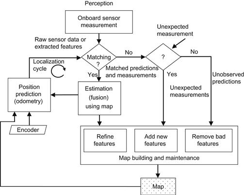
A generic self-explained diagram showing the structure and interconnections of the various functions (operations) for performing SLAM is provided in Figure 12.10.
The three typical methods for implementing SLAM are:
EKF is an extension of Kalman filter to cover nonlinear stochastic models, which allows to study observability, controllability, and stability of the filtered system. Bayesian estimators describe the WMR motion and feature observations directly using the underlying probability density functions and the Bayes theorem for probability updating. The Bayesian approach has shown a good success in many challenging environments. The PF (or as otherwise called, sequential Monte Carlo method) is based on simulation [15]. In the following sections, all these SLAM methods will be outlined.
12.8.2 EKF SLAM
The motion of the WMR and the measurement of the map features are described by the following stochastic nonlinear model [16]:
![]() (12.32a)
(12.32a)
![]() (12.32b)
(12.32b)
where the state vector ![]() contains the m-dimensional position
contains the m-dimensional position ![]() of the vehicle, and a vector
of the vehicle, and a vector ![]() of n stationary d-dimensional map features, that is,
of n stationary d-dimensional map features, that is, ![]() has dimensionality
has dimensionality ![]() :
:
![]() (12.33)
(12.33)
The l-dimensional input vector ![]() is the robot’s control command, and the l-dimensional process
is the robot’s control command, and the l-dimensional process ![]() is a Gaussian stochastic zero-mean process with constant covariance matrix
is a Gaussian stochastic zero-mean process with constant covariance matrix ![]() . The function
. The function ![]() represents the sensor model, and
represents the sensor model, and ![]() represents the inaccuracies and noise. It is also assumed that
represents the inaccuracies and noise. It is also assumed that ![]() is a zero-mean Gaussian process.
is a zero-mean Gaussian process.
Given a set of measurements ![]() for the current map estimate
for the current map estimate ![]() the expression:
the expression:
![]() (12.34a)
(12.34a)
gives an a priori noise-free estimate of the new locations of the robot and map features after the application of the control input ![]() . In the same way:
. In the same way:
![]() (12.34b)
(12.34b)
provides a noise-free a priori estimate of the sensor measurements.
If ![]() and
and ![]() are linear, then the Kalman filter, Eqs. (12.5)–(12.10), can be directly applied. But, in general
are linear, then the Kalman filter, Eqs. (12.5)–(12.10), can be directly applied. But, in general ![]() and
and ![]() are nonlinear in which case we use the following linearizations (first-order Taylor approximations):
are nonlinear in which case we use the following linearizations (first-order Taylor approximations):
![]() (12.35a)
(12.35a)
![]() (12.35b)
(12.35b)
where ![]() ,
, ![]() , and
, and ![]() are the Jacobian matrices:
are the Jacobian matrices:
![]()
Given that the landmarks are assumed stationary, their a priori estimate is:
![]()
Thus, the overall state model of the vehicle and map dynamics is:
![]()
![]()
or
![]() (12.36)
(12.36)
![]() (12.37)
(12.37)
where:
![]() (12.38a)
(12.38a)
![]() (12.38b)
(12.38b)
Using the augmented linearized model for the dynamics of the position and environmental landmarks, we can apply directly the same steps as those given in Section 12.7 for the linear localization problem.
For convenience, we repeat here the sequence of the covariances:
 (12.39)
Under the condition that the pair ![]() is completely observable, the filter covariance tends to a constant matrix
is completely observable, the filter covariance tends to a constant matrix ![]() which is given by the following steady-state (algebraic) Riccati equation:
which is given by the following steady-state (algebraic) Riccati equation:
![]() (12.40)
(12.40)
It is noted that in SLAM the complete observability condition is not satisfied in all cases. Clearly, the steady-state covariance matrix ![]() depends on the values of
depends on the values of ![]() ,
, ![]() and
and ![]() , as well as on the total number
, as well as on the total number ![]() of landmarks. The solution of (12.40) can be found by standard computer packages (e.g., Matlab).
of landmarks. The solution of (12.40) can be found by standard computer packages (e.g., Matlab).
The EKF-SLAM solution is well developed and possesses many of the benefits of the application of the EKF technique to navigation or tracking control problems. However, since EKF-SLAM uses linearized models of nonlinear dynamics and observation models, it leads sometimes to inevitable and critical inconsistencies. Convergence and consistence can only by assured in the linear case as illustrated in the following example.
Example 12.3
Consider a one-dimensional WMR (monorobot) with state ![]() , and a one-dimensional landmark
, and a one-dimensional landmark ![]() as shown in Figure 12.11 [16].
as shown in Figure 12.11 [16].
The WMR’s position error dynamics is:
![]() (12.41)
(12.41)
and the landmarks dynamics is:
![]() (12.42)
(12.42)
The map generated by this system is a single static landmark ![]() . The observation (measurement) model for this landmark is:
. The observation (measurement) model for this landmark is:
![]() (12.43)
(12.43)
where ![]() is the landmark’s measurement error. Equations (12.41)–(12.43) can be written in the standard form of Eqs. (12.2a) and (12.2b), that is:
is the landmark’s measurement error. Equations (12.41)–(12.43) can be written in the standard form of Eqs. (12.2a) and (12.2b), that is:
![]() (12.44)
(12.44)
![]() (12.45)
(12.45)
where:
![]()
For the filtering problem, the term ![]() is just an additive term, and has no influence on the filtered estimate. The filtered estimate is given by:
is just an additive term, and has no influence on the filtered estimate. The filtered estimate is given by:
![]()
Here, the matrix ![]() is equal to:
is equal to:
![]() (12.46)
(12.46)
which has the eigenvalues ![]() and
and ![]() . We see that
. We see that ![]() is always equal to 1 regardless of the filter gain matrix
is always equal to 1 regardless of the filter gain matrix ![]() . Therefore, the filter in this case is only marginally stable (i.e., it performs constant amplitude oscillations). This can easily be verified via simulation. To overcome this problem which is caused by a partially observable system, we can use several techniques to assure complete observability of the pair
. Therefore, the filter in this case is only marginally stable (i.e., it performs constant amplitude oscillations). This can easily be verified via simulation. To overcome this problem which is caused by a partially observable system, we can use several techniques to assure complete observability of the pair ![]() , that is, the matrix:
, that is, the matrix:
 (12.47)
is of full rank ![]() , in which case it is invertible. These methods include [17]:
, in which case it is invertible. These methods include [17]:
• use of fixed global references,
• use of the relative position of the landmark with respect to the position of the robot instead of global positioning.
Therefore, let us assume that we add an anchor in the measurement process of Eq. (12.43) with state ![]() and noise
and noise ![]() . Then, the measurement model of Eq. (12.45) has:
. Then, the measurement model of Eq. (12.45) has:
![]() (12.48)
(12.48)
Now, the gain matrix ![]() becomes:
becomes:
![]() (12.49)
(12.49)
and the matrix ![]() is:
is:
![]() (12.50)
(12.50)
The matrix gain ![]() is given by Eqs. (12.10), (12.7), and (12.8). If
is given by Eqs. (12.10), (12.7), and (12.8). If ![]() and
and ![]() are the standard deviations of
are the standard deviations of ![]() and
and ![]() , respectively, then using the present form of the matrices
, respectively, then using the present form of the matrices ![]() , and
, and ![]() (see Eq. (12.48)), we can verify that:
(see Eq. (12.48)), we can verify that:
 (12.51)
where:
![]() (12.52)
(12.52)
Now, we can see that the eigenvalues of ![]() given by Eq. (12.50) always lie inside the unit circle of the complex
given by Eq. (12.50) always lie inside the unit circle of the complex ![]() plane, and so adding the “anchor” the filter becomes stable.
plane, and so adding the “anchor” the filter becomes stable.
12.8.3 Bayesian Estimator SLAM
In probabilistic (Bayesian) form, the SLAM problem is to compute the conditional probability [18–21]:
![]() (12.53)
(12.53)
where:
![]()
![]()
![]()
represent the history of landmark observations ![]() and the history of control inputs
and the history of control inputs ![]() , respectively. This probability distribution represents the joint posterior density of the landmark locations and WMR state (at time
, respectively. This probability distribution represents the joint posterior density of the landmark locations and WMR state (at time ![]() ) given the recorded observations and control inputs up to and including the time
) given the recorded observations and control inputs up to and including the time ![]() together with the initial state
together with the initial state ![]() of the robot. The Bayesian SLAM is based on Bayesian learning, discussed in Section 12.2.4. Starting with an initial estimate for the distribution:
of the robot. The Bayesian SLAM is based on Bayesian learning, discussed in Section 12.2.4. Starting with an initial estimate for the distribution:
![]() (12.54)
(12.54)
at time ![]() the joint posterior probability, following a control
the joint posterior probability, following a control ![]() and observation
and observation ![]() is computed by Bayes learning (updating) formula (12.15b). The steps of the algorithm are as follows:
is computed by Bayes learning (updating) formula (12.15b). The steps of the algorithm are as follows:
Step 1—Observation Model
Determine the observation model that describes the probability of making an observation ![]() when the WMR location and landmark locations are known. In general, this model has the form:
when the WMR location and landmark locations are known. In general, this model has the form:
![]() (12.55)
(12.55)
Of course, we tacitly assume that once the robot’s location and the map are defined, the observations are conditionally independent given the map and the current WMR state.
Step 2—WMR Motion Model
Determine the motion model of the vehicle which is described by the Markovian conditional probability:
![]() (12.56)
(12.56)
This probability indicates that the state ![]() at time
at time ![]() depends only on the state
depends only on the state ![]() at time
at time ![]() and the exerted control
and the exerted control ![]() , and does not depend on the observations and the map.
, and does not depend on the observations and the map.
 (12.57)
Step 4—Measurement Update
According to Bayes update law:
 (12.58)
Equations (12.57) and (12.58) provide a recursive algorithm for calculating the joint posterior probability ![]() for the WMR state
for the WMR state ![]() and map
and map ![]() at time
at time ![]() using all observations
using all observations ![]() and all control inputs
and all control inputs ![]() up to and including time
up to and including time ![]() . This recursion uses the WMR model
. This recursion uses the WMR model ![]() and the observation model
and the observation model ![]() . We remark that here the map building can be formulated as computing the conditional density
. We remark that here the map building can be formulated as computing the conditional density ![]() . This needs the location
. This needs the location ![]() of the WMR to be known at all times, under the condition that the initial location is known. The map is then produced through the fusion of observations from different positions. On the other hand, the localization problem can be formulated as the problem of computing the probability distribution
of the WMR to be known at all times, under the condition that the initial location is known. The map is then produced through the fusion of observations from different positions. On the other hand, the localization problem can be formulated as the problem of computing the probability distribution ![]() . This requires the landmark locations to be known with certainty. The goal is to compute an estimate of the WMR location with respect to these landmarks.
. This requires the landmark locations to be known with certainty. The goal is to compute an estimate of the WMR location with respect to these landmarks.
The above formulation can be simplified by dropping the conditioning on historical variables in Eq. (12.54) and write the joint posterior probability as ![]() . Similarly, the observation model
. Similarly, the observation model ![]() makes explicit the dependence of observations on both the vehicle and landmark locations. But, here the joint posterior probability cannot be partitioned in the standard way, that is, we have:
makes explicit the dependence of observations on both the vehicle and landmark locations. But, here the joint posterior probability cannot be partitioned in the standard way, that is, we have:
![]() (12.59)
(12.59)
Thus, care should be taken not to use the partition shown in Eq. (12.59) because this could lead to inconsistencies.
However, the SLAM problem has more intrinsic structure not visible from the above discussion. The most important issue is that the errors in landmark location estimates are highly correlated, for example, the joint probability density of a pair of landmarks, ![]() , is highly peaked even when the independent densities
, is highly peaked even when the independent densities ![]() may be very dispersed. Practically, this means that the relative location
may be very dispersed. Practically, this means that the relative location ![]() of any two landmarks
of any two landmarks ![]() may be estimated much more accurately than their individual positions where
may be estimated much more accurately than their individual positions where ![]() may be quite uncertain. In other words, the relative location of landmarks always improves and never diverges, regardless of the WMR’s motion. Probabilistically, this implies that the joint probability density on all landmarks
may be quite uncertain. In other words, the relative location of landmarks always improves and never diverges, regardless of the WMR’s motion. Probabilistically, this implies that the joint probability density on all landmarks ![]() becomes monotonically more peaked as more observations are made.
becomes monotonically more peaked as more observations are made.
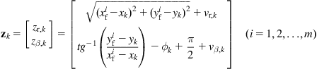
Example 12.4
We consider a differential drive WMR mapping two-dimensional landmarks ![]() ,
, ![]() (Figure 12.12) [16]. The state space of the robot is three dimensional, where the state vector is:
(Figure 12.12) [16]. The state space of the robot is three dimensional, where the state vector is:
![]() (12.60)
(12.60)
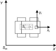
The robot is controlled by a linear velocity ![]() and an angular velocity
and an angular velocity ![]() .
.
Let ![]() be the distance from the center of the wheel axis to the location of the center of projection for any given sensor, and
be the distance from the center of the wheel axis to the location of the center of projection for any given sensor, and ![]() the discrete-time step. The dynamic model of the trajectory of the center of projection of the sensor, which includes the noises
the discrete-time step. The dynamic model of the trajectory of the center of projection of the sensor, which includes the noises ![]() and
and ![]() , is:
, is:
![]() (12.61)
(12.61)
or in detailed form:
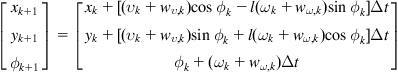 (12.62)
Differentiating Eq. (12.62) with respect to ![]() and
and ![]() , we find the Jacobian matrices:
, we find the Jacobian matrices:
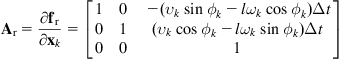
 (12.63)
The measurement model of the sensor (here a laser range scanner) is:
 (12.64)
where ![]() and
and ![]() are the range and bearing of an observed point landmark with respect to the laser center of projection. The position of the ith landmark is
are the range and bearing of an observed point landmark with respect to the laser center of projection. The position of the ith landmark is ![]() and the measurement noises are
and the measurement noises are ![]() and
and ![]() . The Jacobian matrix of this nonlinear model is:
. The Jacobian matrix of this nonlinear model is:
 (12.65a)
where:
![]() (12.65b)
(12.65b)
The measurement model of a global reference, fixed at the origin, for the nonlinear vehicle is:
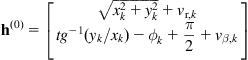
which has the Jacobian matrix:
![]() (12.66)
(12.66)
where ![]() . Thus, the overall measurement matrix
. Thus, the overall measurement matrix ![]() is:
is:
![]() (12.67)
(12.67)
It can be verified that with the addition of the global reference at the origin, the observability matrix ![]() given by Eq. (12.47) is of full rank and so the EKF is stable and provides a steady-state covariance matrix
given by Eq. (12.47) is of full rank and so the EKF is stable and provides a steady-state covariance matrix ![]() (see Eq. (12.40)). This has also been verified experimentally [16].
(see Eq. (12.40)). This has also been verified experimentally [16].
12.8.4 PF SLAM
The purpose of the PF is to estimate the robot’s position and map parameters ![]() (see Eq. (12.53)) for
(see Eq. (12.53)) for ![]() on the basis of the data
on the basis of the data ![]() ,
, ![]() . The Bayes method computes the
. The Bayes method computes the ![]() using the posterior probability
using the posterior probability ![]() . The Markov sequential Monte Carlo (MSMC) method (PF) is based on the total probability distribution
. The Markov sequential Monte Carlo (MSMC) method (PF) is based on the total probability distribution ![]() [18,22,23].
[18,22,23].
Here, the Markov stochastic model given by Eqs. (12.32a) and (12.32b) of the system is described in a probabilistic way as follows [18]:
1. ![]() is a first-order Markov process such that:
is a first-order Markov process such that:
![]() corresponds to
corresponds to ![]() with initial distribution
with initial distribution ![]() .
.
2. Assuming that ![]() are known, the observations
are known, the observations ![]() are conditionally independent, that is,
are conditionally independent, that is, ![]() is described by
is described by ![]() .
.
Particle methods belong to the sampling statistical methods which generate a set of samples that approximate the filtering probability distribution ![]() .2 Therefore, with
.2 Therefore, with ![]() samples, the expectation with respect to the filtering distribution is approximately given by:
samples, the expectation with respect to the filtering distribution is approximately given by:
![]()
where ![]() can give, by the Monte Carlo technique, all moments of the distribution up to a desired degree. The particle method which is mostly used is the so-called sequential importance resampling (SIR) method proposed by Gordon and colleagues [18]. In this method, the filtering distribution
can give, by the Monte Carlo technique, all moments of the distribution up to a desired degree. The particle method which is mostly used is the so-called sequential importance resampling (SIR) method proposed by Gordon and colleagues [18]. In this method, the filtering distribution ![]() is approximated by a set of
is approximated by a set of ![]() particles (multiple copies) of the variable of interest:
particles (multiple copies) of the variable of interest:
![]()
where ![]() are weights that signify the relative quality of the particles, that is, they are approximations to the relative posterior probabilities (densities) of the particles such that:
are weights that signify the relative quality of the particles, that is, they are approximations to the relative posterior probabilities (densities) of the particles such that:
![]()
SIR is a recursive (sequential, iterative) form of importance sampling where the expectation of a function ![]() is approximated by a weighted average:
is approximated by a weighted average:
![]()
One of the problems encountered in PFs is the depletion of the particle population in some regions of space after some iterations. As most of the particles have drifted far enough, their weights become very small (close to zero) and they no longer contribute to estimates of ![]() (i.e., they can be omitted).
(i.e., they can be omitted).
The samples of ![]() are drawn using a proposed probability distribution
are drawn using a proposed probability distribution ![]() . Usually, as proposed probability distribution we select the transition prior distribution
. Usually, as proposed probability distribution we select the transition prior distribution ![]() , which facilitates the computations.
, which facilitates the computations.
The PF algorithm consists of several steps. At each step, for ![]() , we do the following:
, we do the following:
1. Draw from the proposed distribution ![]() samples
samples ![]() :
:
![]()
2. Update the importance (or quality) weights up to a normalizing constant:
![]() (12.68a)
(12.68a)
If as proposed distribution, the prior distribution ![]() is used, that is,
is used, that is, ![]() , the above expression for
, the above expression for ![]() reduces to:
reduces to:
![]() (12.68b)
(12.68b)
3. Compute the normalized weights as:
![]() (12.69)
(12.69)
4. Compute an estimate of the effective sample size (i.e., number of particles) ESS as:
![]() (12.70)
(12.70)
5. If ![]() , where
, where ![]() is a maximum (threshold) number of particles, then perform population resampling as described below.
is a maximum (threshold) number of particles, then perform population resampling as described below.
The PF method can be applied to the mobile robot localization problem.
Actually, we have three phases:
1. Prediction—use a model for the simulation of the effect that a control action has on the set of particles with the noise added (see Eq. (12.32a)).
2. Update—use information obtained from sensors to update the weights such that to improve the probability distribution of the WMR’s motion (see Eq. (12.32b)).
3. Resampling—draw ![]() particles from the current set of particles with probabilities proportional to their weights and replace the current set of particles with this set selecting the weights as
particles from the current set of particles with probabilities proportional to their weights and replace the current set of particles with this set selecting the weights as ![]() .
.
Note 1: Resampling is performed if ESS in Eq. (12.70) is ![]() (see Section 13.13, Phase 3).
(see Section 13.13, Phase 3).
Note 2: A Matlab code for EKF- and PF-based SLAM can be found in:
http://www.frc.ri.cmu.edu/projects/emergencyresponse/radioPos/index.html.
A schematic representation of the PF loop is as shown in Figure 12.13:

We recall that after a certain number of iterations, ![]() , most weights become nearly zero and therefore the corresponding particles have negligible importance. This fact is indeed faced by the resampling process which replaces these low-importance particles with particles of higher importance.
, most weights become nearly zero and therefore the corresponding particles have negligible importance. This fact is indeed faced by the resampling process which replaces these low-importance particles with particles of higher importance.
12.8.5 Omnidirectional Vision-Based SLAM
The main issue in SLAM is that the robot can build a map of the environment and localize its position/posture in this map on the basis of noisy measurements of characteristic points (landmarks) from the images. The measurements of a catadioptric camera are particularly suited for use in conjunction with EKF in which every state variable or output variable is represented by its mean and covariance. The motion of the WMR and the measurements are described by Eqs. (12.32a) and (12.32b), where ![]() and
and ![]() are nonlinear functions of their arguments. The state vector
are nonlinear functions of their arguments. The state vector ![]() at time
at time ![]()
![]() contains the position vector
contains the position vector ![]() of the vehicle, and the vector
of the vehicle, and the vector ![]() of the map features. The disturbances/noises
of the map features. The disturbances/noises ![]() and
and ![]() are assumed Gaussian with zero means and known covariances. The EKF equations involve the Jacobian matrices of
are assumed Gaussian with zero means and known covariances. The EKF equations involve the Jacobian matrices of ![]() and
and ![]() . For the catadioptric camera system, these matrices have been derived in Example 9.4, and can be used to formulate the EKF equations in a straightforward way. Two examples of this application are provided in Refs. [24,25].
. For the catadioptric camera system, these matrices have been derived in Example 9.4, and can be used to formulate the EKF equations in a straightforward way. Two examples of this application are provided in Refs. [24,25].
Example 12.5
In this example, we will develop the full EKF equations for the localization of a unicycle-type WMR using (fusing) two kinds of sensors [26]:
• Encoders on the powered wheels that provide a measure of the incremental rotation angles over a possibly varying sampling period ![]() .
.
• A set of sonar sensors mounted on the platform of the WMR.
The WMR kinematic equations ![]() ,
, ![]() , and
, and ![]() are discretized using the first-order approximation
are discretized using the first-order approximation ![]() , giving the discrete-time model:
, giving the discrete-time model:
 (12.71)
where ![]() (or
(or ![]() for simplicity) and
for simplicity) and ![]() (constant). This model is nonlinear in the state vector:
(constant). This model is nonlinear in the state vector:
![]() (12.72a)
(12.72a)
The control vector is:
![]() (12.72b)
(12.72b)
The disturbance inputs ![]() are zero-mean Gaussian white noises with known identical variances
are zero-mean Gaussian white noises with known identical variances ![]() . The model in Eq. (12.71) can be written in the compact form of Eq. (12.32a):
. The model in Eq. (12.71) can be written in the compact form of Eq. (12.32a):
![]() (12.73)
(12.73)
where:
 (12.74)
with additive disturbance ![]() . The linear approximation of Eq. (12.73) is (see Section 12.8.2):
. The linear approximation of Eq. (12.73) is (see Section 12.8.2):
![]() (12.75)
(12.75)
where ![]() is the current estimate of
is the current estimate of ![]() (based on measurements up to time
(based on measurements up to time ![]() ), and:
), and:
 (12.76a)
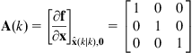 (12.76b)
 (12.76c)
Let ![]() be the coordinates of the ith sonar sensor in the vehicles coordinate frame
be the coordinates of the ith sonar sensor in the vehicles coordinate frame ![]() , and
, and ![]() the orientation angle of the ith sonar in
the orientation angle of the ith sonar in ![]() as shown in Figure 12.14.
as shown in Figure 12.14.

The discrete-time kinematic equations in Oxy of the ith sonar are:
 (12.77)
Now, consider a plane (surface) ![]() as shown in Figure 12.15, and a sonar
as shown in Figure 12.15, and a sonar ![]() with beam width
with beam width ![]() (all sonars are assumed to have the same beam width
(all sonars are assumed to have the same beam width ![]() ). Each plane
). Each plane ![]() can be represented in Oxy by
can be represented in Oxy by ![]() and
and ![]() , where:
, where:
• ![]() is the (normal) distance of
is the (normal) distance of ![]() from the origin
from the origin ![]() of the world coordinate frame.
of the world coordinate frame.
• ![]() is the angle between the normal line to the plane
is the angle between the normal line to the plane ![]() and the Ox direction.
and the Ox direction.
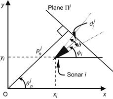
The distance ![]() of sonar
of sonar ![]() from the plane
from the plane ![]() is (see Figure 12.15):
is (see Figure 12.15):
![]() (12.78a)
(12.78a)
![]() (12.78b)
(12.78b)
The measurement vector ![]() contains the encoder and sonar measurements and has the form:
contains the encoder and sonar measurements and has the form:
![]() (12.79)
(12.79)
where ![]() is a Gaussian zero-mean white measurement noise with covariance matrix
is a Gaussian zero-mean white measurement noise with covariance matrix ![]() , and:
, and:
![]() (12.80a)
(12.80a)
![]() (12.80b)
(12.80b)
with ![]() (
(![]() is the number of sonars),
is the number of sonars), ![]() the distance measurement with respect to the plane
the distance measurement with respect to the plane ![]() provided by the ith sonar,
provided by the ith sonar, ![]() (
(![]() is the number of planes), and
is the number of planes), and ![]()
For simplicity, we assume (without loss of generality) that only one sensor and one plane are used (i.e., ![]() and
and ![]() , in which case:
, in which case:
![]() (12.81)
(12.81)
Linearizing the measurement Eq. (12.79) about ![]() , where
, where ![]() is the estimate of
is the estimate of ![]() using measurement data up to time
using measurement data up to time ![]() , and noting that
, and noting that ![]() does not depend on
does not depend on ![]() , we get:
, we get:
![]() (12.82)
(12.82)
![]() (12.83a)
(12.83a)
 (12.83b)
Now, having available the linearized model of Eqs. (12.75) and (12.82), we can use directly the linear Kalman filter Eqs. (12.5)–(12.12). For the robot localization we use the steps described in Section 12.7.1.
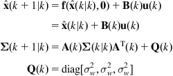 (12.84)
Step 2: Sensor Observation
A new set of sensors’ measurements ![]() is taken at time
is taken at time ![]()
Step 3: Matching
The measurement innovation process:
![]() (12.85)
(12.85)
is constructed.
![]() (12.86a)
(12.86a)
![]() (12.86b)
(12.86b)
![]() (12.86c)
(12.86c)
with ![]() a given symmetric positive definite matrix.
a given symmetric positive definite matrix.
Any valid controller that guarantees the stability of the closed-loop system can be used. Here, a dynamic state feedback linearizing and decoupling controller derived by the method of Example 6.7 will be used [26,27]:
We select the output vector:
![]() (12.87a)
(12.87a)
and differentiate it to obtain:
![]() (12.87b)
(12.87b)
Clearly, ![]() does not influence
does not influence ![]() , and so we introduce a dynamic compensator
, and so we introduce a dynamic compensator
![]() (12.88)
(12.88)
where ![]() is the linear WMR acceleration. Therefore, Eq. (12.87a) takes the form:
is the linear WMR acceleration. Therefore, Eq. (12.87a) takes the form:
![]() (12.89)
(12.89)
Differentiating Eq. (12.89) we get:
![]() (12.90)
(12.90)
where ![]() is the nonsingular decoupling matrix:
is the nonsingular decoupling matrix:
![]() (12.91)
(12.91)
with ![]() .
.
Thus, defining new inputs ![]() and
and ![]() such that:
such that:
![]() (12.92)
(12.92)
and solving Eq. (12.90) for ![]() we get:
we get:
![]()
which is the desired dynamic state feedback linearizing and decoupling controller:
![]() (12.93a)
(12.93a)
![]() (12.93b)
(12.93b)
![]() (12.93c)
(12.93c)
![]() (12.93d)
(12.93d)
Numerical Results—We consider the following values of the system parameters and initial conditions:
![]()
The desired trajectory starts at ![]() ,
, ![]() and is a straight line that forms an angle of
and is a straight line that forms an angle of ![]() with the world coordinate
with the world coordinate ![]() axis as shown in Figure 12.16.
axis as shown in Figure 12.16.
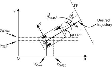
The new feedback controller ![]() is designed, as usual, using the linear PD algorithm:
is designed, as usual, using the linear PD algorithm:
![]()
![]()
Figure 12.17A shows the trajectory obtained using odometric and sonar measurements and the desired trajectory. Figure 12.17B shows the desired orientation ![]() , and the real orientation
, and the real orientation ![]() obtained using the EKF fusion. As we see, the performance of the EKF fusion is very satisfactory.
obtained using the EKF fusion. As we see, the performance of the EKF fusion is very satisfactory.

Figure 12.17 (A) Actual trajectory obtained using both kinds of sensors versus the desired trajectory (![]() ) and (B) corresponding curves for the orientation
) and (B) corresponding curves for the orientation ![]() (
(![]() …) and
…) and ![]() (—).
(—).
However, the experiment showed that the trajectories obtained by pure odometric measurements, and by combined odometric and sonar data are similar. This is perhaps due to modeling reasons. Here, the case of using both sensors was treated jointly by a single EKF. A better picture of the improvement can be obtained by using the sensor fusion process of Figure 12.8 by first computing separately the (local) estimates provided by each individual kind of sensor, and then finding the combined estimate according to (12.31a) and (12.31b) which eliminates the effect of any redundant information.
Further improvement in the accuracy of the state vector estimation can be obtained using the PF approach. This is because the EKF assumes Gaussian disturbances and noise processes which in general is not so, whereas in the PF no assumptions are made about the probability distributions of the stochastic disturbances and noises. In PF, a set of weighted particles (state vector estimates) is employed, which evolve in parallel. Each iteration of the PF involves particle updating and weight updating, and convergence is assured through resampling by which particles with low weights are replaced by particles of high weights. Indeed, simulation experiments using PF for the above sensor fusion system example, with number of particles ![]() , have shown that the PF is superior than the EKF. As the number of particles was increased, better estimates of the WMR state vector were obtained, of course with higher computational effort.
, have shown that the PF is superior than the EKF. As the number of particles was increased, better estimates of the WMR state vector were obtained, of course with higher computational effort.
Example 12.6
It is desired to give a solution to the problem of estimating the leader’s velocity ![]() in a leader–follower vision-based control system (Figure 12.18).
in a leader–follower vision-based control system (Figure 12.18).
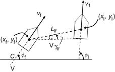
Solution
The image processing algorithms give the range and bearing data [28], that is:
![]() (12.94a)
(12.94a)
![]() (12.94b)
(12.94b)
Differentiating ![]() and
and ![]() we get:
we get:
![]() (12.95a)
(12.95a)
![]() (12.95b)
(12.95b)
where:
![]() (12.95c)
(12.95c)
Defining the angle ![]() as:
as:
![]() (12.96)
(12.96)
and assuming that ![]() and
and ![]() , we find that the state vector under estimation is described by the nonlinear model:
, we find that the state vector under estimation is described by the nonlinear model:
![]() (12.97a)
(12.97a)
where ![]() is a Gaussian stochastic disturbance input process with zero-mean and known covariance matrix and:
is a Gaussian stochastic disturbance input process with zero-mean and known covariance matrix and:
 (12.97b)
The measured output ![]() is:
is:
![]() (12.97c)
(12.97c)
where ![]() is the zero-mean sensor measurement Gaussian noise with known covariance matrix.
is the zero-mean sensor measurement Gaussian noise with known covariance matrix.
Discretizing Eqs. (12.97a)–(12.97c) with first-order approximation and sampling period ![]() gives the nonlinear discrete-time model:
gives the nonlinear discrete-time model:
![]() (12.98a)
(12.98a)
![]() (12.98b)
(12.98b)
where:
 (12.98c)
We will apply the EKF technique to the nonlinear model given by Eqs. (12.98a)–(12.98c) which is linearized, as usual, about the current estimate ![]() to give (see Eqs. (12.32a)–(12.35b)):
to give (see Eqs. (12.32a)–(12.35b)):
![]() (12.99a)
(12.99a)
where the estimate ![]() is based on measurements
is based on measurements ![]() , and:
, and:
 (12.99b)
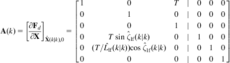 (12.99c)
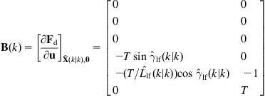 (12.99d)
The measurement Eq. (12.97c) is linear by its own, and can be written as:
![]() (12.100a)
(12.100a)
where:
![]() (12.100b)
(12.100b)
The linear state-space and measurement model given by Eqs. (12.99a)–(12.99d), (12.100a), and (12.100b) has the standard form of Eqs. (12.2a) and (12.2b) or Eqs. (12.75) and (12.82), and so the formulation of the EKF equations is straightforward. As an exercise the reader can write down these equations and write a computer program with proper values of the parameters.
Example 12.7
Given that a sensor is available to measure the range and the bearing of observed landmarks, it is desired to outline an algorithm that updates the pose (position and orientation) of a car-like WMR.
Solution
The algorithm is similar to the velocity estimation algorithm of the previous example. Here, the kinematic model of the car-like WMR is:
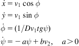 (12.101)
where “![]() ” is the decay parameter of the steering angle
” is the decay parameter of the steering angle ![]() , which is assumed to be constrained as
, which is assumed to be constrained as ![]() , and
, and ![]() is an input gain.
is an input gain.
The control vector is:
![]()
To use the EKF for updating the position and orientation of the WMR, we first discretize (as usual) this model and get (see Eqs. (12.98a) and (12.98b)):
![]() (12.102a)
(12.102a)
 (12.102b)
where ![]() and
and ![]() are zero-mean Gaussian white processes with known covariance matrices
are zero-mean Gaussian white processes with known covariance matrices ![]() and
and ![]() , respectively, and
, respectively, and ![]() is the position of the ith landmark:
is the position of the ith landmark:
![]() (12.102c)
(12.102c)
The output function ![]() is:
is:
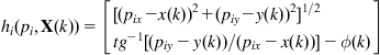 (12.102d)
The function ![]() is given by:
is given by:
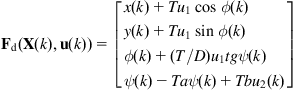 (12.103a)
where:
![]() (12.103b)
(12.103b)
The linearized state and measurement model is found to be:
![]() (12.104a)
(12.104a)
![]() (12.104b)
(12.104b)
where:
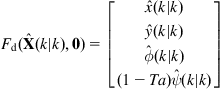


![]()
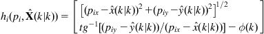

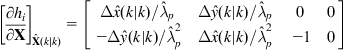
where ![]() ,
, ![]() , and
, and ![]() .
.
Again, the model given by Eqs. (12.104a) and (12.104b) is a standard linear time-varying stochastic model to which the EKF is applied directly. The four steps:
provide the solution (see Section 12.7.1). In the matching step, we can use the ![]() criterion to validate the matching (independence) of each landmark (sensor) measurement. Measurements that do not satisfy this criterion are ignored. It is remarked that the control input
criterion to validate the matching (independence) of each landmark (sensor) measurement. Measurements that do not satisfy this criterion are ignored. It is remarked that the control input ![]() in the term
in the term ![]() of Eq. (12.104a) is assumed to be known (since our aim here is purely the estimation of
of Eq. (12.104a) is assumed to be known (since our aim here is purely the estimation of ![]() ). This input can be selected by a proper method (Chapters 5–9) for achieving a desired control objective as it was done in Example 12.5.
). This input can be selected by a proper method (Chapters 5–9) for achieving a desired control objective as it was done in Example 12.5.
References
1. Papoulis A. Probability, random variables and stochastic processes New York, NY: Mc Graw-Hill; 1965.
2. Meditch JS. Stochastic optimal linear estimation and control New York, NY: Mc Graw-Hill; 1969.
3. Anderson BDO, Moore JB. Optimal filtering Prentice Hall, NJ: Englewood Cliffs; 1979.
4. Borenstein J, Everett HR, Feng L. Navigating mobile robots: sensors and techniques Wellesley, MA: A.K. Peters Ltd; 1999.
5. Adams MD. Sensor modeling design and data processing for automation navigation Singapore: World Scientific; 1999.
6. Davies ER. Machine vision: theory, algorithms, practicalities San Francisco, CA: Morgan Kaufmann; 2005.
7. Bishop RH. Mechatronic systems, sensors and actuators: fundamentals and modeling Boca Raton, FL: CRC Press; 2007.
8. Leonard JL. Directed sonar sensing for mobile robot navigation Berlin: Springer; 1992.
9. Kleeman, L. Advanced sonar and odometry error modeling for simultaneous localization and map building. In: Proceedings of the 2004 IEEE/RSJ international conference on intelligent robots and systems, Sendai, Japan, 2004, p. 1866–71.
10. Betke M, Gurvis L. Mobile robot localization using landmarks. IEEE Trans Rob Autom. 1997;13(2):251–263.
11. Andersen CS, Concalves JGM. Determining the pose of a mobile robot using triangulation: a vision based approach. Technical Report No I. 195-159, European Union Joint Research Center, December 1995.
12. Hu H, Gu D. Landmark-based navigation of industrial mobile robots. Int J Ind Rob. 2000;27(6):458–467.
13. Castellanos JA, Tardos JD. Mobile robot localization and map building: a multisensor fusion approach Berlin: Springer; 1999.
14. Chang KC, Chong CY, Bar-Shalom Y. Joint probabilistic data association in distributed sensor networks. IEEE Trans Autom Control. 1986;31:889.
15. Durrant-Whyte HF. Uncertainty geometry in robotics. IEEE Trans Rob Autom. 1988;4(1):23–31.
16. Vidal Calleja TA. Visual navigation in unknown environments. Ph.D. Thesis, IRI, Univ. Polit. de Catalunya, Barcelona, 2007.
17. Guivant JE, Nebot EM. Optimization of the simultaneous localization and map-building algorithm for real-time implementation. IEEE Trans Rob Autom. 2001;17(3):242–257.
18. Gordon NJ, Salmond DJ, Smith AFM. Novel approach to nonlinear/nonGaussian Bayesian estimation. Proc IEE Radar Signal Process. 1993;140(2):107–113.
19. Rekleitis I, Dudek G, Milios E. Probabilistic cooperative localization and mapping in practice. Proc IEEE Rob Autom Conf. 2003;2:1907–1912.
20. Rekleitis I, Dudek G, Milios E. Multirobot collaboration for robust exploration. Ann Math Artif Intell. 2001;31(1–4):7–40.
21. Bailey T, Durrant–Whyte H. Simultaneous localization and mapping (SLAM), Part I. IEEE Rob Autom Mag. 2006;13(2):99–110 Part II, ibid, (3):108–17.
22. Doucet A, De Freitas N, Gordon NJ. Sequential Monte Carlo methods in practice Berlin: Springer; 2001.
23. Crisan D, Doucet A. A survey of convergence results on particle filtering methods for practitioners. IEEE Trans Signal Process. 2002;50(3):736–746.
24. Rituerto A, Puig L, Guerrero JJ. Visual SLAM with an omnidirectional camera. In: Proceedings of twentieth international conference on pattern recognition (ICPR), Istanbul, Turkey, 23–26 August, 2010, p. 348–51.
25. Kim JM, Chung MJ. SLAM with omnidirectional stereo vision sensor. In: Proceedings of 2003 IEEE/RSJ international conference on intelligent robots and systems, Las Vegas, NV, October, 2003, p. 442–47.
26. Rigatos GG, Tzafestas SG. Extended Kalman filtering for fuzzy modeling and multi-sensor fusion. Math Comput Model Dyn Sys. 2007;13(3):251–266.
27. Oriolo G, DeLuca A, Venditteli M. WMR control via dynamic feedback linearization: design implementation and experimental validation. IEEE Trans Control Sys Technol. 2002;10(6):835–852.
28. Das AK, Fierro R, Kumar V, Southall B, Spletzer J, Taylor CJ. Real-time mobile robot. In: Proceedings of 2001 international conference on robotics and automation, Seoul, Korea, 2001, p. 1714–19.
2For convenience, we drop the dependence on the inputs ![]() .
.