
17
Introduction to Laser Beam Profiling
Introduction
Lasers produce light with many characteristics that are unique compared to other light sources. For example, the monochromatic nature of a laser beam means that it emits photons at a single wavelength with very little energy at wavelengths other than the central peak. The temporal nature of a laser beam enables it to vary from a continuous wave (CW) to an extremely short pulse providing very high power densities. The coherence of a laser enables it to travel in a narrow beam with a small and well-defined divergence or spread. This allows a user to exactly define the area irradiated by the laser beam. Because of this coherence, a laser beam can also be focused to a very small and intense spot, resulting in a highly concentrated energy density. This property makes the laser beam useful for many applications in physics and chemistry and in medical and industrial applications. Finally, a laser beam has a unique spatial intensity profile that gives it very significant characteristics. The beam profile is the quantitative pattern of the distribution of the irradiance across the beam.
Case For Laser Beam Profiling
There are many laser applications in which the beam profile is of critical importance. Because the beam profile is important, it is usually necessary to measure it to ensure that the proper profile exists. For some lasers and applications this may only be necessary during design or fabrication of the laser. In other cases, it is necessary to monitor the laser profile continuously during the process. For example, scientific laser applications often force the laser to its operational limits, and continuous or periodic measurement of the beam profile is necessary to ensure that the laser is still operating as expected. Some industrial laser applications require periodic beam profile monitoring to eliminate scrap produced when the laser beam quality degrades. In medical laser applications, the practitioner often does not have the capability to tune the laser. The laser manufacturer measures the beam profile in the design phase to ensure that the laser provides reliable performance at all times and is responsible for guaranteeing that the spatial beam profile remains stable. However, there are medical uses of lasers, such as photorefractive keratotomy (PRK), for which periodic checking of the beam profile can considerably enhance the reliability of the operation. PRK is an example of laser beam shaping, a process by which the irradiance of the laser beam is changed along its cross section. For this laser beam shaping to be effective, it is necessary to be able to measure the degree to which the irradiance pattern or beam profile has been modified by the shaping medium.
The importance of the beam profile is that the total energy density at the target, the spatial uniformity, and the collimation of the light are all affected by it. In addition, the propagation of the beam through space is significantly affected by the beam profile. Figure 17.1 shows three laser beam profiles among the variety of spatial profiles that can exist. Because almost every laser has a unique beam profile, it is essential to measure the profile to ensure that the spatial distribution is appropriate for the application.
Brief History Of Spatial Laser Beam Profiling
Several nonelectronic methods of laser beam profile measurement have been used ever since lasers were invented. The first and by far the simplest and least expensive method is observance of a laser beam reflected from a wall or other object. The problem with this method is that the response of the human eye is logarithmic and can differentiate only among orders of magnitude differences in light irradiance. In a single order of magnitude, a well-trained observer can distinguish only 8–12 shades of gray. Thus, it is nearly impossible for a visual inspection of a laser beam to provide anything even approaching a quantitative measurement of the beam size and shape. The beam width measurement by eye may have as much as 100% error.
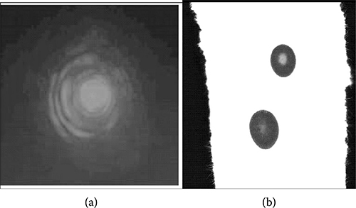
Figure 17.2a is a photograph of a HeNe laser beam reflected from a wall (photographic film has even less dynamic range than the human eye). The image appears to be a very intense beam at the center, but a very large amount of structure far out from the center. This structure, however, which one might mistake as part of the laser beam, is less than 1% of the total energy in the beam. Yet, the eye and the film give erroneous importance to this region of low energy. In addition, the eye cannot really distinguish structure in a laser beam with less than 2-to-1 magnitude variation.
Figure 17.1
Various laser beam profiles: (a) HeNe, (b) excimer, and (c) nitrogen ring laser. Each has a unique and different spatial beam profile. (Courtesy of Ophir-Spiricon Inc.)

Burn paper, photographic film, and some polymers, such as Kaptan, have also been used for making beam profile measurements. Figure 17.2b illustrates thermal paper irradiated by a laser beam. The burn paper typically has a dynamic range of only three levels: unburned paper, blackened paper, and paper turned to ash. Sometimes, skilled operators can distinguish in between these levels and increase the dynamic range to five levels. The main objection to this manual method is that the spot size is highly dependent on the duration of the irradiance of the beam. With longer exposure times, the center of the burn spot may not change, but the width of the darkened area could change by 50% or more.
Wooden tongue depressors and burn spots on metal plates have also been used because the depth of the burn can often yield additional insight into the laser irradiance profile. Sometimes, operators learn from experience with these burn spots so that a specific pattern is indicative of an acceptable beam profile for a specific application. However, this measurement system is archaic, crude, and nonquantitative; subjective to the experience of the operator; and therefore quite unreliable.
Figure 17.2
(a) Photograph of a HeNe laser beam as (b) it appears on a scattering surface and burn spots on paper. The human eye is logarithmic and will incorrectly determine the true beam width. (Courtesy of Ophir-Spiricon Inc.)
Another method involves the use of fluorescing plates, typically used to view CO2 laser beams. Energy from the laser quenches the fluorescing property roughly proportional to the intensity, and this pattern can be viewed by the technician. However, fluorescing plates have limited dynamic range, which adds to the dynamic range problem already described when viewing reflected beams.
As requirements for laser beam profiling became more stringent, electromechanical methods were developed. They generally involved the use of a single-element electronic or thermoelectronic detector to measure the total power of the beam and a sharp blade on a mechanical translation device that could accurately block the beam. This knife-edge method would allow the scientist to record the points on the translation stage at which the power reaching the detector was reduced by known amounts, typically 10% and 90% of the total. The difference in the location of the knife edge at these two points was then given as the beam width.
Once this method was in general use, several other calculated beam widths were defined, such as full width at half maximum; 1/e and 1/e2; percentage of peak; and percentage of energy. The proliferation of these measurements was that they all yielded different beam widths, even on the same laser beam. This prompted one researcher to comment that “Measuring a beam width is like trying to measure the width of a cotton ball with a caliper.”
The International Organization for Standardization (ISO) has standardized the measurement of beam width under their specification 11146, which has made the measurement of laser beam characteristics unambiguous and identical for all beams. The standard measurement D4σ, commonly called the second moment, is clearly defined and can be made on all types of laser beams.
Spatial Profiling Requirements
Of course, modern beam-profiling techniques make spatial laser beam profiling quite simple compared to the early days of the laser. However, unless one takes particular care in defining the conditions under which the measurement is to be made, the results will not be representative of the laser beam. In general, the following must be given thorough consideration before a spatial beam measurement is performed:
The type of laser to be measured.
What kind of laser is it?
What is the main wavelength of the laser?
The operating condition of the laser.
Is the laser running in pulsed mode or CW mode?
The total average power of the laser.
If CW, then what is the total average power (expressed in watts)?
The energy per pulse of the laser.
If the laser is pulsed, then what is the energy per pulse (expressed in joules)?
In addition, what is the pulse rate (expressed in pulses per second or hertz)?
What is the pulse duration, expressed in time units (milliseconds to femtoseconds)?
The anticipated beam diameter (expressed in millimeter).
If the beam is parallel (e.g., unfocused) or focused.
Once these issues have been properly addressed, it is then possible to define the instrumentation that can be used to spatially profile the laser.
Types Of Beam-Profiling Systems
Mechanical Scanning Devices
One of the earliest methods of measuring laser beams electronically was using a mechanical scanning device. This usually consists of a rotating drum containing a knife edge, slit, or pinhole that moves in front of a single-element detector. This method provides excellent resolution, sometimes to less than 1 μm. The limit of resolution is set by diffraction from the edge of the knife edge or slit, and roughly 1 μm is the lower limit set by this diffraction. These devices can be used directly in the beam of medium-power lasers with little or no attenuation because only a small part of the beam is impinging on the detector element at any one time. Most of the time, the scanning drum is reflecting the beam away from the detector.
However, mechanical scanning methods are suitable only for CW (not pulsed) lasers. They also have a limited number of axes for measurement (usually two) and integrate the beam along those axes. Thus, they do not give detailed information about the structure of the beam perpendicular to the direction of travel of the edge. However, rotating drum systems with knife edges on seven different axes provide multiple axis cuts to the beam. This can assist somewhat in obtaining more detailed information about the beam along the various axes. These beam profile instruments are adaptable for work in the visible, ultraviolet (UV), and infrared (IR) by using different types of single-element detectors for the sensor. In addition, software has been developed that will display two-dimensional (2D) and three-dimensional (3D) beam profiles as well as fairly detailed quantitative measurements from the scanning system. This software now exists in the PC-based Windows operating system for easy use.
A variation of the rotating drum system includes a lens mounted in front of the drum (Sasnett, 1990). The lens is mounted on a moving axis and thus focuses the beam to the detector at the back side of the drum. By moving the lens in the beam, a series of measurements can be made by the single-element detector that enables calculation of M 2. A photograph of a seven-axis measuring instrument and readout is given in Figure 17.3.
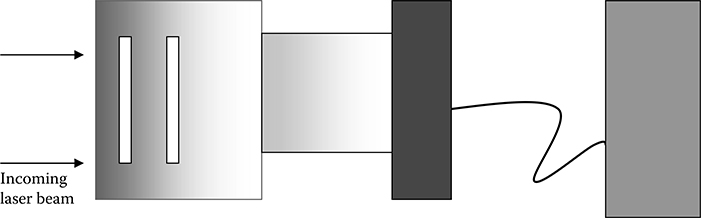
For electronic laser beam profile analysis, it is nearly always necessary to attenuate the laser beam, at least to some degree, before measuring the beam with an electronic instrument. The degree of attenuation required depends on two factors. The first is the irradiance of the laser beam being measured. The second is the sensitivity of the beam profile sensor. Figure 17.4 shows a typical setup for when the maximum amount of attenuation is required before the sensor measures the beam.
Typically when measuring the beam profile of higher-power lasers (i.e., in excess of 50–100 W), the irradiance of the beam is sufficient to destroy most sensors that might be placed in the beam path. Therefore, the first element of Figure 17.4, the beam-sampling assembly, is typically used regardless of the beam-profiling sensor. It should be noted, however, that there are some beam-profiling sensors that can be placed directly into the path of a high-power beam of 10 kW for short periods of time under very specific operating conditions.
For mechanical scanning instruments, the beam-sampling assembly is usually sufficient to reduce the signal from high-power lasers down to the level that is acceptable by such instruments. For mechanical scanning instruments, lasers up to 50 W can be measured directly without using the beam-sampling assembly because the rotating drum blocks the energy from the laser during most of the duty cycle of the sensor; therefore, high power is not placed on the sensing element.
Figure 17.3
Typical readout from seven-axis system.
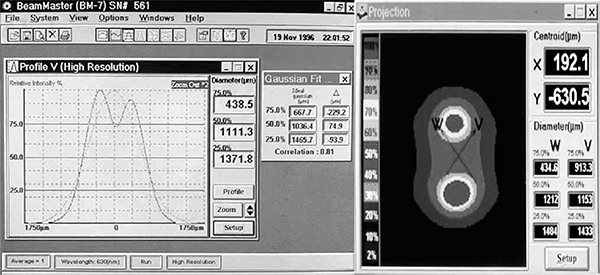
Figure 17.4
Schematic diagram for beam profiling.

Another mechanical scanning system consists of a rotating needle that is placed directly in the beam. This needle has a small opening that allows a very small portion of the beam to enter the needle. A 45° mirror at the end of the needle reflects the sampled part of the beam to a single-element detector (see Figure 17.15 later in the chapter). The needle is both rotated and translated across the beam to sample it, much as a fax machine scans a document. The advantage of a rotating needle system is that it can be placed directly in the beam of high-power industrial lasers for near- and mid-IR wavelengths. It introduces a small distortion in the process beam, so many users restrict its use. In addition, the translation of the needle can be made extremely small for focused spots or large for unfocused beams. It has, however, some characteristics of the rotating drum mentioned. Specifically, it is not very useful for pulsed lasers because of the synchronization problem between the position of the needle and the timing of the laser pulse. These rotating needle systems also have extensive computer processing of the signal with beam displays and quantitative calculations in Windows-based systems.
Camera-Based Imaging Systems
Camera-based imaging systems are used to provide simultaneous, whole 2D laser beam measurements in real time. Unlike mechanical scanning instruments, camera-based systems work with both pulsed and CW lasers. Most laser beam-profiling applications occur from the UV (193-nm) region to the near-IR at 1.1 μm. For these applications, silicon-based cameras are ideal because of their low cost and high resolution. Figure 17.5 illustrates the detail in the structure of a laser made capable with charge-coupled device (CCD) technology. Other types of cameras will image in the x-ray and deep UV regions, the far-IR above 1.4 μm into the terahertz band, and beyond, above 2000 μm.
One drawback of camera-based systems is that, in direct imaging, the resolution of the beam width calculations is often limited to approximately the size of the pixels. In CCD cameras, this is roughly 4.4 μm, and for most IR cameras the pixel size ranges from 25 to 100 μm. However, a focused spot can be reimaged with lenses to provide a larger image for viewing on the camera, which provides a resolution down to approximately 1 μm. In this case, the resolution for a camera-based system is limited by diffraction in the optics.
Figure 17.5
Highly structured laser beam measured with a charge-coupled device camera and shown in both two and three dimensions. (Courtesy of Ophir-Spiricon Inc.)
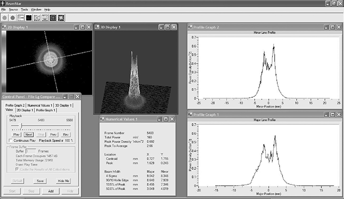
Cameras are now available with a variety of interfaces to connect to a computer. Current computer software packages provide very detailed 2D and 3D beam displays, as shown in Figure 17.6. The software (Figure 17.7) also provides very sophisticated numerical analysis of the beam profile.
A camera-based beam-profiling system includes a computer; an interface (Frame grabber, FireWire, USB-II, or similar) to digitize the signal; and software to control the camera, display the beam profiles, and make quantitative calculations (Figure 17.4). A silicon CCD camera can be used from 190 to 1300 nm, covering the UV to the near-IR range. A pyroelectric, lead sulfide (PbS or Vidicon), indium gallium arsenide (InGaAs), or other camera is used for wavelengths to about 2.2 μm. CCD cameras have extremely sensitive sensors and can measure nanowatts of power. Other types of cameras can image from about 1 μW. Therefore, laser beam attenuation is almost always needed before it enters the camera. Often, the beam is either too large or too small, and beam sizing optics or other techniques must be used to size the beam for the camera. Figure 17.4 illustrates schematically the steps necessary for proper beam profiling.
Figure 17.6
Examples of scientific-based beam-profiling software. The two-dimensional and three-dimensional images are displayed in real time, giving the user a powerful intuitive tool for visualizing and diagnosing the beam structure. (Courtesy of Ophir-Spiricon Inc.)
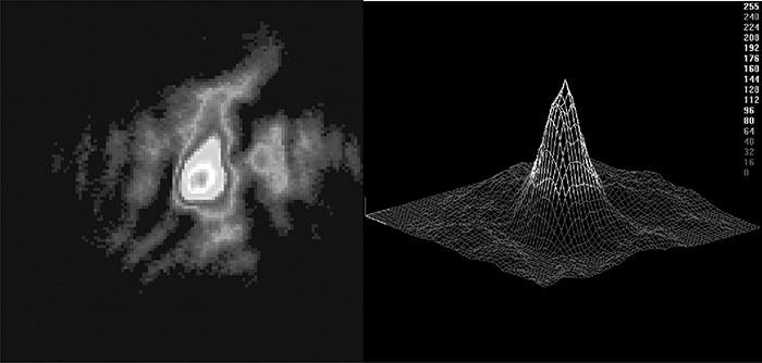
Figure 17.7
Example of industrial beam-profiling software. (Courtesy of OphirSpiricon Inc.)
Wavelength Dependencies of Camera-Based Systems
Selection of the proper camera technology for each application is critical to proper imaging. Each type of camera has advantages and disadvantages for various applications. The most common type of camera for laser beam diagnostics uses a silicon-based sensor. These cameras consist of two types, charge injection devices and CCDs. Silicon-based cameras cover the wavelength range from 190 nm to 1.3 μm when the protective glass window is removed, which would otherwise attenuate the UV and also cause interference fringes in the image because of the parallel surfaces of the window. These cameras are fairly inexpensive, and because they cover the visible region, they are the most common cameras used. At slightly longer wavelengths, lead sulfide (Vidicon) sensors cover the region from the visible to 2.2 μm. A newer solid-state camera technology based on an InGaAs sensor also covers the range from visible to about 2 μm. The most common cameras for IR lasers of wavelengths longer than 1 μm are pyroelectric solid-state cameras. These are fairly low resolution at 124 × 124 pixels with 100-μm elements but cover the wavelength range from 1 μm to beyond 2000 μm, as well as work in the UV range from 190 to 350 nm. In addition, ferroelectric (microbolometer) sensors have been tried for the range of 4–12 μm, but their baseline characteristics have not been satisfactory for quantitative measurements, and they are seldom used for laser beam profiling. Finally, there are many cooled IR cameras that can be used for the wavelength range from 1 to about 12 μm. In general, their initial cost and the use of liquid nitrogen make them unsuitable for all but the most demanding applications.
In addition, there are many considerations when choosing a camera for beam profiling, especially when using pulsed laser sources in the near-IR region (1064 nm) as many sensors will produce a ghost image when the photons from the laser excite both the charge-coupled sensor and the silicon substrate. This technology is constantly evolving, and the user is advised to contact the major beam-profiling vendors to ensure that the latest camera sensors are used for best results.
How To Choose A System Based On Applications
The real challenge in beam profiling is how to determine the optimum combination of attenuation, sizing, sensors, and analysis for each application. Fortunately, Figure 17.4 enables both the experimentalist and industrial user alike to make the correct choices with a minimum of error. Recall the spatial beam-profiling considerations at the beginning of the chapter; it is now possible to choose the instruments best suited for the application.
The most important selection will be the detector as it must be capable of imaging the wavelength of the laser tested. Once the detector has been selected, the size of the beam to be measured will determine if the user must either enlarge or shrink the beam to fit onto the detector. In particular, the user must pay attention to the propagation of the beam under consideration (i.e., if the beam is focused or unfocused). Next, the average power of the laser output will then determine the amount of attenuation necessary. Finally, the user may select the best software package for the application.
The market for laser beam profiling is quite active and crowded. For this reason, the user should rely on major manufacturers of these instruments for their expertise so that a valid measurement may be made. If adherence to the ISO specification is required, it should be the responsibility of the experimentalist to verify that the vendor understands this requirement.
Temporal Beam Analysis
Another critical parameter of the laser is its temporal profile, that is, the power or energy delivered during a single pulse of the laser. The temporal profile can be as important in laser processing as the spatial profile. Most laser manufacturers can shape a temporal laser pulse. This process has many applications in industry, such as treating metal components to improve strength and corrosion resistance. Other applications of temporal pulse shaping include drilling via holes in multilayer printed circuit boards. It follows that one needs to measure the temporal profile to verify that the laser is responding properly to the input waveform.
For most lasers, this measurement is fairly simple to perform. All that is required is a fast photodiode with a response that lies in the wavelength range of the laser and a suitable recording device such as an oscilloscope.
Width Measurements And Why They Are Important
The most fundamental laser profile measurement is the beam width. It is a measurement of primary significance because it affects many other beam parameters. The beam width gives the size of the beam at the point where it is measured. However, this can be significant in terms of determining the correct diameters of the elements in the optical train. Measurement of beam width is also a part of measuring the divergence of the laser beam, which is significant in predicting what size the beam will be at some other point in the optical train. The beam width is critical for the performance of most nonintegrating beam-shaping systems. Statistical measurement of the width of the beam is also a significant factor in determining the stability of the laser output. Finally, measurement of the beam width is essential in calculating the M 2 of the laser. In spite of its significance, the beam width is sometimes a very difficult measurement to perform accurately.
Recent ISO standards (Sasnett and Johnston, 1991; Siegman, 1990a–c, 1993; Woodward, 1990) have defined a second moment beam width, abbreviated D4σ, that for many cases gives the most realistic measure of the actual beam width. The equation for the second moment beam width is given in Equation 17.1. Equation 17.1 is an integral of the irradiance of the beam multiplied by the square of the distance from the centroid of the beam and then divided by the integrated irradiance of the beam. This equation is called the second moment because of the analogy to the second moment of mechanics and is abbreviated D4σ because it is the diameter at ±2σ, which is equivalent to ±1/e2 for Gaussian beams. This second moment definition of a beam width enables a user to accurately predict what will happen to the beam as it propagates, its real divergence, and the size of the spot when the beam is focused.
|

|

where (x – X) and (y – Y) are the distances to the centroids in the X and Y axes, respectively.
Sometimes, there are conditions of laser beams for which the second moment measurement is not an appropriate measurement. This is particularly true when there are optical elements in the beam smaller than twice the 1/e2 beam width, which cause diffraction of part of the energy in the beam. This diffraction will put energy further out into the wings of the beam, which, when measured by the second moment method, will cause a measurement of the beam width much larger than is significant for the central portion of the beam. In Equation 17.1, the (x – X)2 term overemphasizes small signals far from the centroid. This requires judgment on the part of the users regarding whether measurement of this diffracted energy is significant for their application. If the diffracted energy, which typically diverges more rapidly than the central lobe, is not significant, it is possible to place a physical or software aperture around the main lobe of the beam and make second moment measurements only within this aperture and disregard the energy in the wings. However, if the application is dependent on the total amount of energy and it is important to know that part of this energy is diffracted, then one would want to place this aperture such that it includes all the beam energy in making the calculation.
When using a camera-based profiler, a number of camera characteristics must be carefully considered and accounted for in accurately measuring beam width. Among these considerations is the signal-to-noise ratio, that is, the magnitude of the beam signal relative to the background noise in the camera. The amount of attenuation used for the camera is usually adjusted to enable the peak pixel in the camera to be as near to saturation as possible without overdriving the camera. If the beam width is very small in a very large field of camera pixels, the beam may represent a very small amount of signal compared with the random noise of all the pixels. Proper treatment of this noise must be performed.
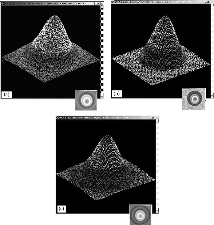
The camera baseline offset is another factor that must be accurately controlled. Because the energy of a laser does not abruptly fall to zero but trails off to a width roughly four times the standard deviation, or twice the 1/e2 width, there is a lot of low-power energy that must be accounted for in accurately measuring the width of the beam (Roundy, 1993, 1996; Roundy et al., 1993). (The percentage of total energy in a Gaussian beam is 68% in ±1σ, 95% in ±2σ, and 99.7% in ±3σ. Nevertheless, experiments have shown that as an aperture cuts off the beam at less than ±4σ, the measured beam width begins to decrease.) Correct and incorrect baseline controls are shown in Figure 17.8a through c. In Figure 17.8a, the baseline is set too low, and the digitizer cuts off all the energy in the wings of the beam. The beam is seen to rise out of a flat, noiseless baseline. This means that without the wings of the laser beam, a measurement would report a width much too small. In Figure 17.8b, the baseline offset is too high, as seen by observing the beam baseline relative to the small corner-defining mark. In this case, the software will interpret the baseline as part of the laser beam. A calculation of beam width will be much too large. In Figure 17.8c, the baseline is set precisely at zero. Both positive and negative noise components are retained out beyond the wings of the beam where there is no beam energy. The software will interpret the average of the positive and negative signals as nearly zero.
Figure 17.8
(a) The baseline is well above the zero mark, and the beam width is calculated 24% too large. (b) The beam rises out of a flat background, which shows clipping of the wings of the beam by the analog-to-digital converter. The width is calculated 26% too small. (c) The baseline is calibrated correctly, as seen by the wings just going to zero. (Courtesy of Ophir-Spiricon Inc.)
Because the energy of the beam in the wings can have a significant effect on the width measurement, it becomes necessary to be able to characterize the noise in the wings of the beam. Both the noise components that are above and the noise components that are below the average noise in the baseline must be considered. The noise below the average baseline is called negative noise. Any software that does not correctly account for this negative noise will not yield correct beam width calculations.
Since the size of the beam measurement is affected by the total amount of laser beam energy relative to the noise of the camera, it has been found that software apertures placed around the beam can have a very strong effect in improving the signal-to-noise ratio. For a nonrefracted beam, an aperture approximately two times the 1/e2 width of the beam can be placed around the beam, and all noise outside the aperture can be set to zero in the calculation. This greatly improves the relative signal-to-noise ratio when small beams are measured in a large camera field.
M2 And Why It Is Useful
Increasingly, M 2, or k in Europe (k = 1/M 2), has become important in describing the beam propagation characteristics of a laser beam (Borghi and Santarsiero, 1998; Chapple, 1994; Herman and Wiggins, 1998; Johnston, 1990, 1998; Lawrence, 1994; Sasnett and Johnston, 1991; Siegman, 1990a–c, 1993; Woodward, 1990). In many applications, especially those in which a Gaussian beam is the desired profile, M 2 is the most important characteristic describing the relative characteristics of the beam. Figure 17.9 shows the essential features of the concept of M 2 as defined by Equations 17.2a and b. As shown in Figure 17.9, if a given input beam of width Din is focused by a lens, the focused spot size and divergence can be readily predicted. If the input beam is a pure TEM00, the spot size equals a minimum defined by Equation 17.2a and d00 in Figure 17.9. However, if the input beam Din is composed of modes other than pure TEM00, the beam will focus to a larger spot size, namely, M 2 times larger than the minimum, as shown mathematically in Equation 17.2b and d0 in Figure 17.9. The ISO definition for the beam propagation factor of a laser beam uses M 2 as the fundamental measurement parameter:
|

Figure 17.9
Curve showing M2. (Characteristics and equations relating M2 to the beam-focused spot size.)

|

where λ is the wavelength of the laser, f the focal length of the lens, and Din the width of the input beam at the waist.
In measuring and depicting M 2, it is essential that the correct beam width be defined. The ISO standard and beam propagation theory indicate that the second moment is the most relevant beam width measurement in defining M 2. Only the second moment measurement follows the beam propagation laws, so that the future beam size will be predicted by Equations 17.2a and b. Beam width measured by other methods may or may not give the expected width in different parts of the beam path.
M2 is not a simple measurement to make. It cannot be found by measuring the beam at any single point. Instead a multiple set of measurements must be made as shown in Figure 17.10, in which an artificial waist is generated by passing the laser beam through a lens with known focal length. One additional requirement is to measure the beam width exactly at the focal length of the lens. This gives the divergence of the beam. Other measurements are made near the focal length of a lens to find the width of the beam and the position at the smallest point. The values of beam widths along the propagation axis are fitted to a hyperbolic function using a cubic fit. The coefficients of the cubic fit are then used to solve the M 2 equation in Figure 17.2b. In addition, measurements are made beyond the Rayleigh range of the beam waist to confirm the divergence measurement. With these multiple measurements, one can then calculate the divergence and minimum spot size; then, going backward through Equation 17.2b, one can find the M 2 of the input beam.
Figure 17.10
Multiple measurements made for M2.

The measurement shown in Figure 17.10 can be made in a number of ways. In commercial instruments, shown in Figures 17.11 and 17.12, a detector is placed behind a rotating drum with knife edges, and then the lens is moved in the beam to effect ively enable the measurement of the multiple spots without having to move the detector. This instrument works extremely well as long as the motion of the lens is in a relatively collimated part of the laser beam. However, if the beam is either diverging or converging in the region where the lens is moving, the resultant M 2 measurement can be misleading. It also violates ISO 11146: The lens to laser must remain fixed!
Figure 17.11
M2 measuring instrument and readout based on scanning slit.
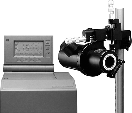
Figure 17.12
Schematic diagram of a slit-based M2 measuring instrument.

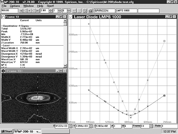
The ISO (1993) method for measuring M 2 requires the lens at a fixed position, then making multiple detector position measurements as shown in Figure 17.10. This can be done by placing a lens on a rail and then moving the camera along the rail through the waist and through the far-field region. There are commercially available instruments that perform this measurement automatically without having to manually position the camera along the rail. One of these is shown in Figure 17.13, where the lens and the camera are fixed, but folding mirrors are mounted on a translation table and moved to change the path length of the beam after the focusing lens. A typical readout of an M 2 measurement is shown in Figure 17.14. In this case, a collimated laser diode was measured, which gave a much greater divergence in the X axis than in the Y axis. The steep V curve displayed is the X axis of the beam coming to a focus following the lens. The more gradual curve is the focus of the less-divergent Y axis. Notice that while for most of the range the X axis has a wider beam width, at focus the X axis focuses smaller than the Y axis. Also, the X-axis M 2 was 1.46, whereas the Y-axis M 2 was only 1.10. The M 2 reported in the number section is calculated from the measurements of the beam width at the focal length (by fitting the data to the hyperbolic function and extracting the coefficients, then solving the equation), the minimum width, and the divergence in the far field according to the equations in the ISO standard.
Figure 17.13
Schematic diagram of a camera-based instrument with fixed-position lens for measuring M2.
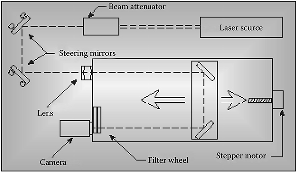
Figure 17.14
M2 measurement display and calculation readout.
One of the difficulties of accurately measuring M2 is accurately measuring the beam width. This is one of the reasons so much effort has been made to define the second moment beam width and create algorithms to accurately make this measurement. Another difficulty in measuring this beam width is that the irradiance at the beam focus is much greater than it is far from the Rayleigh length. This necessitates that the measurement instrument operates over a wide dynamic range. Multiple neutral density filters are typically used to enable this measurement. An alternative exists with cameras or detectors that have extremely wide dynamic range, typically 12 bits, so that sufficient signal-to-noise ratio is obtained when the irradiance is low, still not saturating the detector near the focused waist.
There are some cases when M 2 is not a significant measure of the functionality of a laser beam. For example, flat-top beams for surface processing typically have a very large M 2, and M 2 is not at all relevant to the functionality of the beam. Nevertheless, for many applications in nonlinear optics, industrial laser processing, and many others, the smallest possible beam with the M 2 closest to 1 is the ideal. Some flat-top beam shapers are designed for an input Gaussian beam; then, the M 2 of the input beam should be very close to 1, and the beam widths should closely match the design width.
Measurement At Focus
Until recently, measuring the spatial profile of a focused beam was limited to two technologies: the spinning slit and spinning wire or hollow-needle instruments. Rotating slit measurements use a cylinder on which one or more microscopically thin slits have been placed. The beam is directed onto the cylinder, and a single-element detector assembles a major and minor axis beam profile from the intensity–time relationship, which correlates to spatial location. The spinning wire/hollow-needle method (Figure 17.15) depends on either a micron-size pinhole in a hollow tube or an equally small reflector at the end of a needle that passes through the beam, and again the spatial image is assembled from the repeated passes of the wire or needle through the beam, in much the same way as a fax machine assembles a replica of the original on a remote machine (Green, 2004).
A new accessory has been developed that can be attached to almost any CCD camera-based system that performs the attenuation steps in an extremely short distance, so that the array can be positioned at or near the focus of the beam. The system uses standard quartz wedges, which reflect only 4% of the incoming energy and pass the rest through the bulk of the wedge material. By placing additional wedges in proximity to each other, enough attenuation can be achieved by the time the focused spot arrives at the camera array. In this manner, the beam profile of the focused spot as well as just before and just after the focus can be displayed in real time. In addition, for shorter focal length focusing lenses, a negative lens can be attached to translate the focus further away, so the focus can be imaged on the camera. Figure 17.16 shows this device attached to a CCD camera.
Figure 17.15
Spinning wire, hollow-needle, and slit devices all make composite images, taking as much as 10 seconds per image. The gaps in the image occur when a pulsed laser is not emitting. (Courtesy of Primes GmbH, Prometec GmbH.)

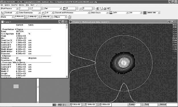
It can be seen from Figure 17.17 that small focused spots can be imaged even with short (fast) focal length lenses. In this case, a 75-mm focal length lens produced a spot of only 65 μm.
Location of Focus and Why It Is Critical to Processes
The location of the focused spot and its size is critical to every process. Most processes are dependent on the irradiance of the beam squared. Since the irradiance is proportional to the area of the beam, it follows that the irradiance of the beam is proportional to the radius of the beam squared. Thus, the irradiance of the beam at the point of contact at the process is proportional to the radius to the fourth power. The beam width then plays a critical role in the size of the processing window. The ability to measure the actual focused beam width and its location can provide the user with new insights into the ability of the beam to produce the proper process ability.
Figure 17.16
Negative lens and quartz wedges allow imaging of focused spots on a charge-coupled device camera. (Courtesy of Ophir-Spiricon Inc.)

Figure 17.17
A 65-μm spot imaged from a 75-mm focal length lens. (Courtesy of OphirSpiricon Inc.)
Newer techniques are being developed almost monthly. The scientist and industrial user alike will no doubt wish to contact the major vendors of laser beam-profiling instrumentation to determine the best solution for each application.
REFERENCES
Borghi, R., and Santarsiero, M. (1998). Modal decomposition of partially coherent flat-topped beams produced by multimode lasers. Opt. Lett., 23: 313–315.
Chapple, P. B. (1994). Beam waist and M2 measurement using a finite slit. Opt. Eng., 33: 2461–2466.
Green, I. (2004). Process monitoring of industrial CO2 lasers. In Proceedings of the 2004 Advanced Laser Applications Conference and Expositions, eds. D. Roessler and N. Uddin, 107–113. ALAC: Ann Arbor, MI.
Herman, R. M., and Wiggins, T. A. (1998). Rayleigh range and the M 2 factor for Bessel–Gauss beams. Appl. Opt., 37: 3398–3400.
International Organization for Standardization. (1993). Test methods for laser beam parameters: Beam widths, divergence angle and beam propagation factor (Document ISO/11146).
Johnston, T. F. Jr., (1990). M-squared concept characterizes beam quality. Laser Focus World, 26: 173–183.
Johnston, T. F. Jr., (1998). Beam propagation (M 2) measurement made as easy as it gets; The four-cuts method. Appl. Opt., 37: 4840–4850.
Lawrence, G. N. (1994). Proposed international standard for laser-beam quality falls short. Laser Focus World, 30: 109–114.
Roundy, C. B. (1993). Digital imaging produces fast and accurate beam diagnostics. Laser Focus World, 29: 117.
Roundy, C. B. (1996). Twelve-bit accuracy with an 8-bit digitizer. NASA Tech Briefs, p. 55H.
Roundy, C. B., Slobodzian, G. E., Jensen, K., and Ririe, D. (1993). Digital signal processing of CCD camera signals for laser beam diagnostics applications. Electro Optics, 23: 11.
Sasnett, M. W. (1990). Characterization of Laser Beam Propagation. Coherent ModeMaster Technical Notes.
Sasnett, M. and Johnston, T. F. Jr., (1991). Beam characterization and measurement of propagation attributes. SPIE, 1414, 21–32.
Siegman, A. E. (1990a). Conference on Laser Resonators. Los Angeles, CA: SPIE/OE LASE ’90.
Siegman, A. E. (1990b). Conference on Lasers and Electro-Optics. Anaheim, CA: CLEO/ IQEC.
Siegman, A. E. (1990c). New developments in laser resonators. SPIE, 1224: 2–14.
Siegman, A. E. (1993). Output beam propagation and beam quality from a multimode stable-cavity laser. IEEE J. Quantum Elec., 29: 1212–1217.
Woodward, W. (1990). A new standard for beam quality analysis. Photon. Spectra, 24: 139–142.