Chapter 6

Foundations of Logic Programming

6.1. Specifications and programming

The most important task of a programmer (at least till now) can be characterized as filling the gap g below:

Specification of a problem (Cannot be run) ← g → Program (Can be run)

Logic programming (LP) tends to reduce this gap (and possibly obtain g = 0) when the specification is given in a logical language (or a language close to a logical one).

It envisions calculus as a controlled deduction. This is related to the paradigm:

In LP, the emphasis is put on what the program computes and paying as little attention as possible to how it computes. It is a declarative form of programming (as opposed to imperative programming).

We give a first glimpse of such a type of programming.

EXAMPLE 6.1.– Imagine that in the following graph, we want to know whether there are paths from A to I, and if so, which ones.

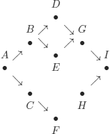
a) We describe the graph using a unary predicate (which corresponds to a property).

Att(x): x is attainable

Premises

Att(A); % Must not be forgotten!

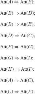
The conclusion:

Two essential questions:

i) which inference rule(s) should we use for deduction?

ii) with what strategy(ies) (forward chaining, backward chaining, others)?

In all cases, it is simple to deduce that in this graph, there are two paths from A to I paths that cannot be found if Att(A) is forgotten.

b) We describe the graph using a binary predicate (that corresponds to a relation):

Path(x, y): there is a path from x to y

As far as questions (i) and (ii) given above are concerned, we decide¹ to use:

i) the resolution rule (the conclusion is also called a question). As usual, the conclusion is negated and we try to derive (contradiction);

ii) backward chaining with the following rules on the stack for the resolvents: we always resolve the first clause in the order 1,2,3…, with the last resolvent obtained (at the beginning, the question) and on the last literal that was pushed (at the beginning, the first literal of the question).

1)	Path(A, B)
2)	Path(A, C)
3)	Path(B, D)
4)	Path(B, E)
5)	Path(C, F)
6)	Path(D, G)
7)	Path(E, G)
8)	Path(G, I)
9)	Path(H, I)
10)	Path(x, y) V Path(x, z) V Path(z, y)	% non-elementary path
11)	Path(A, I)	% (neg) question
12)	Path(A, z) V Path(z, I)	(11,1) — (10, 1) {x ← A, y ← I}
13)	Path(B, I) memorize(12,1) — (2,1)	(12,1) – (1,1) {z ← B}
14)	Path(B, z) Path(z, I) (13, 1) — (10,1) {x1 ← B, y1 ← I}
15)	Path(D, I) memorize(14,1) — (4,1)	(14,1) — (3,1) {z ← D}
16)	Path(D, z) Path(z, I) (15,1) — (10,1) {x2 D,y2 ← I}
17)	Path(G, I)	(16,1) — (6,1) {z ← G}
18)		(17,1) — (8,1)

Note that, as was mentioned in section 5.7.1, each time clause 10 was used, its variables were renamed.

If we want to find all solutions, we need to return to the memorized choices.

REMARK 6.1.– (FOL and databases). In a travel agency, the flights that connect cities are represented as a graph, with vertices representing cities and edges representing direct flights between the cities (labelled by, say, .

We will say that a connection between two cities is acceptable if we can go from one to the other with at most two stops (i.e. three direct flights).

We want to answer questions of the form:

Acceptable-flight(city-a, city-b);

We specify the notion of acceptability in FOL:

by applying the rules used in the proof of theorem 5.3 to transform a formula into a clausal form, we obtain:

which is a Horn clause. By adding this clause to the program describing the graph of flights, we could answer any question on acceptable flights.

EXAMPLE 6.2.– We proceed with a well-known example for computer scientists: appending two lists.

We will use the fact that every list is a tree, for example, the list [a, b, c] is represented by the tree:

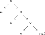
where o denotes the list constructor cons; for example, cons(a[b, c, d]) = [a, b, c, d] and of course, nil denotes the empty list.

Predicates (and logical formulas in general) do not deliver values (as functions do). When we want to mention an object (such as the list obtained by appending the list called x and the list called y), we need to name it:

The program also needs to know that if we add an element to the head of list x, then it will be at the head of list z:

The logic program for append is the following (with o replaced by f for the sake of notational coherence, see definition 4.1).

1)

2)

2 reads: if appending list x to list y yields list z, then appending cons(u, x) to y yields the list cons(u, z).

Similar to resolution, we do not write the prefixes:

and

that are always implicit.

We now ask the question

We prove that the answer is yes for the given specification of append by deducing it by resolution (after having negated the conclusion, i.e. the question):

3)

4)

5)

6)

Logic as a programming language is not limited to answering yes or no, it also has the usual capabilities of languages.

The question we will ask will be:

EXAMPLE 6.3.– Instead of the resulting list, we write a variable in which we will recover (if it exists) the list mentioned in the question above.

3)

4)

5)

6)

REMARK 6.2.– As a side effect of deduction, that answers yes, such an object exists, the unification algorithm used in the resolution rule allows us to construct the list we were looking for:

REMARK 6.3.– Since we are specifying relations, the distinction between input and output parameters (as for functions) is of no interest. It is thus natural to ask questions such as:

We obtain as an answer:

6.2. Toward a logic programming language

We also introduce a syntax that is commonly used in practice (others exist):

The intuitive meaning being:

A →; means A is given or, to prove A there is nothing to do.

A → B₁… B_n; means to prove (solve the problem) A it suffices to prove (solve) the goals B₁ …B_n.

→ B₁… B_n; means we must prove the goals B₁… B_n.

Proving a conclusion (answering a question) boils down to finding, or, equivalently, deleting all the goals of the question.

In a clause (also called a rule):

A is the head of C or left-hand side of C,

B₁ …B_n the tail or body of C or right-hand side of C.

Procedure LP can be considered as an abstract interpreter of the Prolog language.

From now on, we will assume that all logic programs are run with LP.

EXERCISE 6.1.– The strategy that is used by LP may provoke surprises. These “traps” are easy to correct when we are aware of them. This is the object of the following exercise.

a) In what is called the cube world, we define the relations on top(x, y) and above(x,y).

We assume the following state of the world:

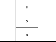
The following specification is proposed for this world:

on top(a, b) →; % i.e. a is on top of b

on top(b, c) →; % i.e. b is on top of c

above(x, y) → on top(x, y); % if x is on top of y, then x is above y.

But this specification is incomplete, as a cube can be above another without being on top of it (for example, a is above c).

Which one of (*) or (**) below must complete the program?

(*) above(u, v) → above(u, z) on top(z, v);

(**) above(u, v) → on top(u, z) above(z, v);

To answer, consider the question:

above(c, a);

and analyze the answers given by LP in each case.

b) Give, as a tree, the trace of the execution of LP with the program:

1) p(a, b)→;

1) P(c, a)→

1) P(x, y) → P(x, z) P(z, y); % transitivity

and the question:

P(u, b);

The syntax of the question has been adapted to existing software.

The question in (b) (and similarly for (a)) can be interpreted as:

– The problem is to know whether there exist objects in relation via P with b;

or, as we used to do in the analysis of reasonings:

– We negate the conclusion, i.e. , and if the reasoning is correct, we must produce.

REMARK 6.4.– We can imagine (and this has indeed been studied and experimented) an interpreter that uses parallelism to handle non-determinism.

With the program:

and the question:

a sequential interpreter does not find any solution and does not halt.

Whereas an interpreter using an AND parallelism (i.e. searching simultaneously for the solution to all the goals of the question) halts without finding a solution, which is normal because it is impossible to solve Q(c).

With the program:

and the question:

a sequential interpreter does not find any solution and does not halt.

Whereas an interpreter using an OR parallelism (i.e. searching simultaneously for all the solutions to one goal of the question) finds a solution.

6.3. Logic programming: examples

EXERCISE 6.2.– Assuming that and elementary arithmetic operations are not incorporated into the interpreter, give the logic programs corresponding to:

a) add (x, y, z): x + y = z

b) mult (x, y, z): x × y = z

c) less (x, y): x < y

d) divides (x, y): x divides y, with mathematical notations, x | y (examples: divides (3, 15), divides (2, 8) divides (3, 10))

e) prime(x): x is a prime number.

EXERCISE 6.3.– Assuming that N and elementary arithmetic operations are not incorporated into the interpreter, give a logic program that permits us to define the relation:

fibonacci(n, x): the value fibonacci(n) is x.

DIGRESSION 6.1.– (regular expressions). Let Σ denote an alphabet (i.e. a finite set of symbols).

The set of regular expressions (r.e.) on Σ is defined as the smallest set such that:

i) ∅ is a r.e.;

ii) the set {} is a r.e. % e denotes the empty string;

iii) if a Σ then {a} is a r.e.

iv) if R and S are r.e., then R S, (R + S), RS, and R* are r.e. (R* is called the Kleene closure)

where:

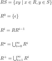
By convention, for singletons, we identify {} with .

EXERCISE 6.4.– Given the following logic program:

1) fact(0,1)→;

2) fact(n +1, (n +1) × y) → fact(n, y);

3) fact(u, v)

where , , γ, below denote the following substitutions (obtained by application of the resolution rule):

and y' take the renaming into account

(2.1) — (3,1) = {u ← n +1, ν ← (n + 1) × y}

Characterize all possible runs of the program using a r.e. that expresses the sequence of substitutions that are applied.

EXERCISE 6.5.– In a commonly used LP language, lists are represented as:

[a, b, c, …,d]

[a₁,a₂,…,a_n | X]: a_i (1 ≤ i ≤ n) is the ith element in the list, and X is what remains.

Define the following predicates (relations) in this language:

a) append (x, y, z): List z is the concatenation of lists x and y;

b) reverse (x, y): List y is list x reversed;

c) palindrome (x): List x is a palindrome;

d) member (x, y): x is a member of list y;

e) subset (x, y): x is a subset of y (where sets are represented by lists);

f) consec (u, v, x): elements u and v are consecutive in list x.

Can we do classical algorithmic in LP?

EXAMPLE 6.4.– (syntactic analysis). Give a logic program that recognizes the words of the grammar whose production rules are:

% This rule does not specify how to associate symbols in the string

We write f (a, b) : a • b % string concatenation

Word(c);

(*) Word(f(a,f(x,b))) → Word(x);

If we want to know whether the word aacbb, which is written as:

a • ((a • (c • b)) • b)

belongs to the language generated by the grammar, we ask the question

Word(f(a,f(f(a,f(c,b)),b)));

that the interpreter will transform into:

Word(f(a,f(c,b)));
Word(c);

and answer:

yes

Note that if we ask the following question:

Word(f (f (a,c), b)), i.e. fortheword acb written: (a • c) • b

the answer will be

no!

This answer may seem surprising at first, but is “normal” as no particular property has been assumed on the functions denoted by functional symbols, in this case associativity (which is known to hold for •, see unification algorithm, section 4.2).

If we wanted a correct answer to this second question, we would have had to write clause (*) as follows:

Word(f(f(a,x),b)) → Word(x);

but in this case, the first question would have resulted in a surprising answer!

Another logic recognition program that avoids these problems would be:

Word(c);
Word(z) → append([a|x], [b], z) Word(x);

In example 9.22, we give another version that is very similar, but uses string constraints, for which there is no problem to be handled by the user.

REMARK 6.5.– If we had had a unification algorithm capable of handling associative functions, i.e. functions f with the property:

We would not have obtained two different answers, depending on the way the symbols in the word were associated.

EXAMPLE 6.5.– (sorting).

sort(x,y) → perm(x,y) ord(y);

% sort(x,y): list y is the sorted list obtained from list x.

% perm(x,y): list y is a permutation of list x.

% ord(y): list y is an ordered list.

perm([], [])→;
perm(z, [x|y]) → delete(x,z,u) perm(u,y);

% delete(x,z,u): u is the list obtained after deleting element x from list z.

delete(x, [x|y], y)→;
delete(x, [y|z], [y|u]) → delete(x,z,u);
ord([])
ord([x])
ord([x,y|z]) → x <= y ord([y|z]);

Other versions:

EXAMPLE 6.6.–

sort(x,y) → perm(x,y) ord(y);
perm([], [])
perm([e |x], z) → insert(e,y,z) perm(x,y);

% insert(e,y,z): list z is obtained by inserting element e in list y

insert(e,x, [e|x])→;
insert (e,[u|x], [u|y]) → insert(e,x,y);

Another one:

EXAMPLE 6.7.–

sort([], [])
sort([u |x], y) → insert(u,z,y) sort(x,z);
insert (x, [], [x])
insert(x,[u |y], [u |z]) → u<x insert (x,y,z) ;
insert(x,[u | y],[x,u | y]) → x<=u;

% is equivalent to [x|u|y]

REMARK 6.6.– This last logic program corresponds to the insertion sort: we remove an element from the list (here the first one), sort the rest of the list and reinsert the element that was removed, while respecting the order.

EXERCISE 6.6.– Give the logic program corresponding to the quick-sort algorithm: we select an element e in a list and divide the list into two sublists, the elements that are smaller than e and those that are greater than e, then e is prefixed by the sorted list of elements that are smaller than e and suffixed by those that are greater than e.

EXERCISE 6.7.– Give the logic program corresponding to the bubble sort algorithm: we test if two adjacent elements are not in the correct order. If so, they are swapped. We repeat the operation until no additional swap is necessary.

EXAMPLE 6.8.– (automaton). We want to define a program that recognizes the words that are accepted by an automaton.

An automaton is defined by a 5-tuple:

where:

Q: set of states;

Σ: vocabulary;

: Q × Σ → Q;

q₀: initial state;

F: set of final states.

For the following automaton (that accepts (ab)*), with initial state q₀ and final state q₀

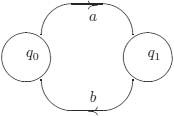
where strings are represented as lists, the program is (q, x, y, z, u) denote variables):

1) initial(q0)→;
2) final(q0)→;
3) delta(q0, a, q1) →;
4) delta(q1,b, q0)→;
5) accepted-string(x) → initial(q) accept(q,x) ;
6) accept(q, []) → final(q) ;
7) accept(q, [x |y]) → delta(q,x,q1) accept-next (q1,y) ;
8) accept-next(q1,[z |u]) → delta(q1,z,q0) accept(q0,u);

a question could be, for example:

accepted-string([a,b,a,b,a,b]);

6.3.1. Acting on the execution control: cut “/”

In principle, it is not necessary in logic programing to know how a program is executed. However, in reality, it is necessary to control executions, which is why imperative characteristics have been introduced into this declarative framework. The cut rule is not very elegant, but is extremely useful, although it must be used very carefully.

The definition given in the use manual is the following:

The “/” is a parasite that can only occur among the terms that make up the righthand side of a rule (in particular, in the question). The choices that remain to be examined and that the deletion (it is always deleted) of “/” removes are as follows:

– the other rules that have the same head as that of the rule where “/” occurs.

– the other rules that could have been used to erase the terms occurring between the beginning of the tail and “/”.

If we represent the execution tree:

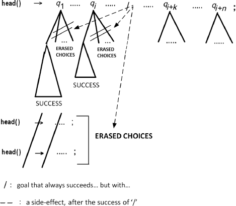
/ : goal that always succeeds… but with…
–-–: a side-effect, after the success of '/'

EXAMPLE 6.9.– (from the manual). The program:

colour (red) →;
colour (blue) →;
size (big) →;
size (small) →;
choicel([x,y]) → colour(x) size(y);
choicel(«that’s all») →;
choice2([x,y]) → / colour(x) size(y);
choice2(«that’s all»)
choice3([x,y]) → colour(x) / size(y);
choice3(«that’s all») →;
choice4([x,y]) → colour(x) size(y) /;
choice4(«that ’ s all») →;

gives the following answers to the asked questions:

choicel(u);
{u= [red,big]}
{u= [red,small]}
{u= [blue,big]}
{u= [blue,small]}
{u= «that’s all»} choice2(u);
{u= [red,big]}
{u= [red,small]}
{u= [blue,big]}
{u= [blue,small]}
choice3(u);
{u= [red,big]}
{u= [red,small]}
choice4(u);
{u= [red,big]}
choicel(u) /;
{u= [red,big]}.

It is not hard to show how useful the cut is; some examples are given below:

6.3.1.1. Translation of imperative structures

For several reasons (for example, because they are more natural, such as in the case of inputs/outputs), we can translate well-known control structures:

if P then Q else R:

if-P-then-Q-else-R → P/Q;

if-P-then-Q-else-R → R;

If P succeeds (is erased), the cut erases the choice of the second rule and problem Q is considered. If P cannot be erased, problem R will be considered.

while R do Q:

P(X) → R(X) /;

P(X) → Q(X,Y) P(Y);

EXERCISE 6.8.– Give the execution trace of the program:

1) R(4) →;
2) 2. Q(1,2) →;
3) 3. Q(2,3) →;
4) 4. Q(3,4) →;
5) 5. P(X) → R(X) /;
6) 6. P(X) → Q(X,Y) P(Y)

with the question:

p(1)

Combination with the predefined predicate repeat.

Here is a predicate that may seem strange if we only think of using it by itself:

repeat →;
repeat →; repeat;

…but here is an example that makes it less strange:

read-spaces (‘ ‘ c) → repeat in-char(c) dif(c,‘ ‘) /;
read-spaces (c,c)→

In this program, in-char (t) : read a character from the input stream.

EXAMPLE 6.10.– (set operations). We represent sets as lists.

member(x,y) → append(u,[x|z], y) ;

other program

member (x, [x|y])→;
member (x, [z|y]) → member (x,y);
non-member(x,[]) →;
non-member(t, [u|x]) → dif(t,u) non-member(t,x) ;
subset ([],x)→;
subset ([z|x], y) → member (z,y) subset (x,y);
inter ([], x, [])→;
inter ([x|u], y, [x|z]) → member (x,y) / inter (u,y,z) ;
inter ([x|u], y,z) → inter (u,y,z) ;
union([], x,x)→;
union([x|u], y, z) → member (x,y) / union(u,y,z) ;
union([x|u], y, [x|z]) → union(u,y,z);

6.3.2. Negation as failure (NAF)

The negation problem is a very delicate problem (including from a philosophical point of view). For example, what can we say about a goal (predicate, problem) that we know we will not be able to prove with the data at our disposal? A solution would be to say “we do not know”.

Another solution is to use the closed world assumption: if we are sure that we cannot prove P (which prevents infinite searches), we conclude P.

This second possibility is the possibility that was chosen. It corresponds to the addition of the rule:

(Here, “no P” means: after an exhaustive search and halting).

Usual implementation of negation in Prolog:

not(Z) → Z / fail;
not(Z)→;

where Z is a predicate variable, meaning that it is mapped to predicates and

fail:: predicate (goal) that always fails (that cannot be erased).

Using not, we can give another definition of if…then… else:

if-P-then-Q-else-R → P Q; if-P-then-Q-else-R → not(P) R;

The choice that was made to treat negation may seem natural, but it leads to several problems, as illustrated in the following examples and exercises.

EXAMPLE 6.11.– The program:

p → not (q) % equivalent to p ∨ q (if not is identified with )

with the question

p;

succeeds, but this means that from p ∨ q, we can deduce p !

EXAMPLE 6.12.

1) correctalg(algol)→;
2) correctalg(algo2)→;
3) correctalg (algo3)→;
4) correctalg(algo4)→;
5) costlyalg(algol)→;
6) costlyalg(algo4)→;
7) reasonablealg(X) → not(costlyalg(X)) ;

with the question:

correctalg(X) reasonablealg(X);

the answer is:

{X = algo2 }
{X = algo3 }

…but with question:

reasonablealg(X) correctalg(X);

the answer is no, as shown by the execution tree:

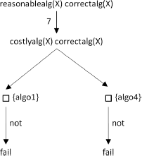
EXERCISE 6.9.– Give the answers to the following questions:

a)

1) man(adam)→;
2) woman(x) → not(man(x));
q1) woman(adam) ; % question 1
q2) woman(eve) ; % question 2
q3) woman(x) eq(x, eve) ;% question 3

% see definition of eq in exercise 6.10 (b).

b)

1) even(0)→;
2) even(s(s(x))) → even(x);
3) odd(s(0))→;
4) odd(s(s(x))) → not(even(x)) ;
q1) even(y); % question 1
q2) odd(y); % question 2

EXAMPLE 6.13.– (beware of non-termination!). We want to write a program that detects whether there is a path from one vertex to another in the graph below (compare with example 6.1).

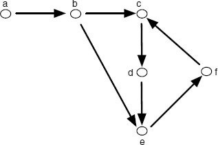
The program that describes the graph and gives the definition of a path is the following:

edge(a,b)→ ;
edge(b,c)→ ;
edge(c,d)→ ;
edge(b,e)→ ;
edge(d,e)→ ;
edge(e,f)→ ;
edge(f,c) → ;
path(x,x)→ ;
path(x,y) → edge(x,z) path(z,y);

It seems obvious that this program is correct, meaning that it describes the world and the desired relations between objects in this world. It is correct, but…let us see what the interpreter LP does (which, as long as there are potential solutions, keeps trying to find them).

We ask the question:

path(a,f);

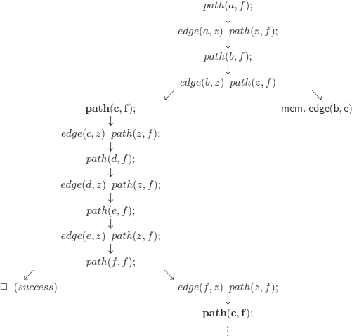
A solution is to replace the last two clauses by the clauses:

path(x,x,t) → ; % t: list of visited nodes
path(x,y,t) → edge(x,z) not(member(z,t)) path(z,y,[z 	]) ;

and the question would then be:

Patch(a,f,[]);

EXERCISE 6.10.– Simulate the interpreter to show that the answers are indeed those given below.

a) consider the program:

1) r(aa)→;

2) q(X) → not(r(X));
3) p(X) → not(q(X));

the question:

p(aa);

succeeds

the question:

p(X)

succeeds and gives as a result the empty substitution (when a goal fails, substitutions are not memorized, which is a reasonable choice).

b) There exists in Prolog a predicateeq (T1,T2), that can be evaluated, and has the following effect when T1 and T2 are variables, say X and Y

eq(X,Y):if X and Y have been linked to the same term, true else if Y (respectively, X) is not yet linked, then it is linked to the same term as X (respectively, Y) else false.

(This does not correspond to usual equality, see section 9.1).

Consider the program:

1) eq(X,X)→;
2) p → not(eq(X,1)) eq(X,2);

the question:

p;

fails.

It should succeed (with X=2)

the question:

not(p);

succeeds.

EXERCISE 6.11.– Give a logic program for the relation merge(X,Y,Z): Z is a sorted list of integers obtained by merging the two sorted lists of integers X and Y.

6.3.2.1. Some remarks about the strategy used by LP and negation as failure

A program containing clauses such as (*) below causes problem at the execution of the program, because it artificially introduces a possibility of non-termination.

The recommended solution is quite natural.

EXAMPLE 6.14.– a) If a program contains the clauses:

(*)cc(X,Y) → cc(Y,X);
cc(s,t) → clause-queue;

with s,t: terms

replace (*) by:

cc(t,s) → clause-queue;

b) If a program contains the clauses:

(*) circ(Y,Z,X) → circ(X,Y,Z)
circ(s,t,u) → clause-queue;

with s, t, u: terms

replace (*) by:

circ(u,s,t) → clause-queue;
circ(t,u,s) → clause-queue;

EXAMPLE 6.15.– (evaluation of formulas). We can sometimes use NAF to evaluate a logical formula in a database that defines the predicates occurring in the formula.

The (very simple) idea is that if we identify not with and the question A₁ A₂… A_n not (B)

– fails then the formula A₁ ∧ A₂ ∧ … ∧ A_n B is evaluated to T;

– succeeds then the formula A₁ ∧ A₂ ∧ … ∧ A_n B is evaluated to F.

For example, if in the database:

3) p(3) → ; 6) q(2,2) → ;

we want to evaluate the formulas:

a) ∀x∀y.F (x) ∧ Q(x, y) F (y)

and:

b) ∀x∀y∀z.Q(x, y) ∧ Q(y, z) ∧ Q(x, z)

Hence, (a) is a valid formula in this world.

Formula (b) is therefore not valid. We could retrieve the substitution:

that corresponds to the counterexample:

6.3.2.2. Can we simply deduce instead of using NAF?

EXAMLPLE 6.16.– (completion (Clark)). The program:

math-class(E106) → ;
math-class(E108) →;

will answer no to the question

math-class(E201);

Using the NAF rule.

To deduce (without any other rule than resolution) this conclusion, we must explicit what is assumed by NAF:

and:

E106 ≠ E108

E106 ≠ E 201
E108 ≠ E 201 E108 ≠ E106
E201 ≠ E106
E201 ≠ E108

The program in clausal form (non-Horn) would then be:

1) math — class(E106)

2) math — class(E108)

3) math — class(x) ∨ (x = E106) ∨ (x = E108)

% Clause 3 is not a Horn clause

4) (E106 = E108)

5) (E106 = E 201)

6) (E108 = E 201)

7) (E108 = E106)

8) (E201 = E106)

9) (E201 = E108)

And we would ask the question

math — class(E201);

we negate the conclusion to obtain:

10) math — class(E201)

and by resolution:

11) E201 = E106 ∨ E201 = E108 (3,1) — (10,1)

12) E201 = E108 (11,1) — (8,1)

13) (12,1) — (9,1).

REMARK 6.7.– (on the utility of studying logic programming). Together with the fact that there are many direct applications that are easy to imagine, starting with examples that have already been seen, the study of the principles of LP is very useful as a first step toward the study of ontology languages (see section 1.2 and digression 8.1), in particular, the so-called description logics in which knowledgebases are made of assertions (i.e. properties of individuals) and terminological axioms (i.e. complex descriptions). The descriptions are specified with unary and binary predicates.

The analogy to LP is obvious.

In the domain of databases, there exists a family of languages (Datalog) based on rules that are clauses (with some restrictions) of FOL. They represent a very important domain of study and can be considered as a “natural” extension of LP.

Datalog perfectly illustrates the deep relationship that exists between logic and computer science.

6.4. Computability and Horn clauses

At this point, the reader who has already written programs in so-called functional languages (Lisp, Scheme, etc.) has probably noticed the similarities between programs in these languages (or simply between the definitions of functions with equations, such as factorial, fibonacci, etc.) and logic programs.

Furthermore, when presented with a new language, say, , it is natural to wonder what its expressive (and computational) power is, in other words, if it enables us to define (and compute) all computable functions.

One way of answering this question is to show that can be used to encode a Turing machine or Markov algorithms, etc. or that it can be used to encode operations that permit us to capture all computable functions (minimization, etc.).

We will choose this way of proceeding, as it will enable us to show the computational power of Horn clauses, and at the same time relate functional programming and LP (also called predicative programming or relational programming).

We first briefly recall the definition of a function that is finitely definable by equations.

We will add to (see signatures in definition 5.1) the constant 0 and the unary function s (for successor), and we shall use the notion of terms (see definition 4.1) on the modified signature, which will be sufficient to suit our needs.

Natural numbers (which are necessary to define functions ) will be denoted by s⁽ⁿ⁾(0).

The variable domain will be the terms of the form s⁽ⁿ⁾(0) (0 ≤ n).

The equations that will occur in the definitions will be term equations, defined on the new signature, with all their variables universally quantified. We shall impose that the subterms t_i (1 ≤ i ≤ n_i) of one of the terms in the equations, say fⁿⁱ_i (t₁,…, t_ni), only contain the functional symbols 0 and s. The (unique) function conventionally denoted by f_i is the function defined by the equational system.

An equational system is a finite set of equations.

We denote the equational systems (and the equations) by (for the sake of readability, we omit the exponent representing the arity; this does not incur any confusion).

f₁,…, f_n and , respectively, represent the set of function symbols and the set of variables that occur in the equations.

DEFINITION 6.1.– (functions definable by equations). A function f_i is finitely definable by an equational system iff there exists an equational system ε such that:

– (meaning that f₁,…, f_n satisfy all the equations in the system);

–for any set of variables , there exists a finite set such that:

and this set uniquely determines

The following theorem (the proof of which can be found in textbooks on computability) characterizes the set of computable functions by functions defined by equational systems.

THEOREM 6.1.– Every recursive function is finitely definable by an equational system.

EXAMPLE 6.17.– (length of a list). We add to the signature (i.e. to ) the function symbols nil, length, cons, add.

length(nil) = 0

length(cons(u, v)) = add(length(v), 1) % we write 1 instead of s(0).

The relationship between equational definitions and computability is established by theorem 6.1, but what is the relationship between these definitions and Horn clauses and their expressive power?

The first key remark is that an equation can be expressed as an implication, in the form of a Horn clause:

Rule I:

with A_i (1 ≤ i ≤ n) and B equational literals (i.e. literals for which the predicate symbol is =), with arguments that are terms of depth 1 or 2 (or 0 or 1 depending on the conventions, see definition 4.2). These terms are called flat terms, meaning that they are of the form:

where

x_i, y: variables (universally quantified) or constants.

The second key remark is that, to obtain flat terms it suffices to name them.

We show how rule I can be used on example 6.17.

1) length(nil) =0 % as nil is a constant, the equation has the desired form

2)

Hence, 2. can be rewritten as:

2')

To get to a logic without equality, we use (the only if part of)

Rule II:

f (x) = y iff F(x,y)

For the example on the length of a list, this yields:

EXAMPLE 6.18.– (length of a list, Horn clauses without =). (We use the syntax from section 6.2)

Length(nil,0)→;

Length(u | v, z) → Length(v,y) Add(y, 1,z); % where u | v is another way of writing cons(u, v)

In a constraint LP language (see section 9.2), the second clause could be written:

Conclusion: rules I and II provide a mechanical way of getting from equational definitions to Horn clauses without equality, which proves that the latter permit us to compute all computable functions.

REMARK 6.8.– The first proof of computability with Horn clauses was produced in 1975-1976. The proof technique consisted of showing that a Turing machine could be encoded with Horn clauses.

More precisely, it was proved that if a function is computable by a Turing machine, then it is computable with Horn clauses containing at most one negative literal (and at most one functional symbol).

An immediate corollary is that the class of Horn clauses is undecidable.

---

1 This decision corresponds to the choice that was made in the most famous of all LP languages: Prolog.