Chapter 12

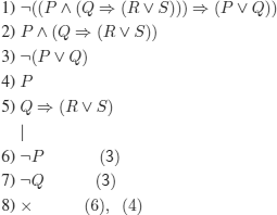
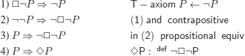
Solutions to the Exercises

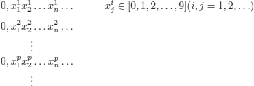
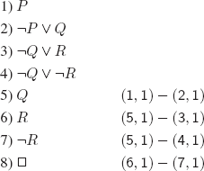
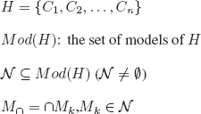
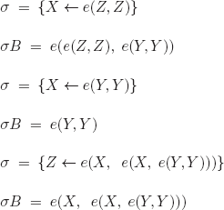
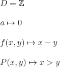
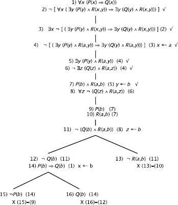
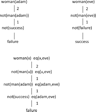
EXERCISE 3.1.– We can represent an interpretation as a subset of Π, with the elements of this subset being the propositional symbols that are evaluated to T in the interpretation.

There are 2^ℵo subsets of Π; hence, there is an uncountably infinite number of interpretations for PL.

A more detailed proof.

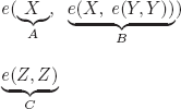
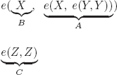
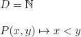
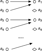
Every interpretation I can be represented by the graph of the function defining it:

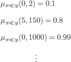
There are infinitely many interpretations, take for example (l ):

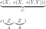
Now if we assume that the set of all interpretations in PL is denumerable, then they can be enumerated (i ):

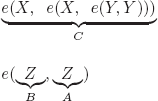
Consider the interpretation defined as follows:

This interpretation is different from every I_i in the list we assumed we were able to construct, at least for the couple (P_i, *).

Therefore, assuming that the set of interpretations for PL is denumerable leads to a contradiction. The set of all interpretations of PL is therefore uncountably infinite.

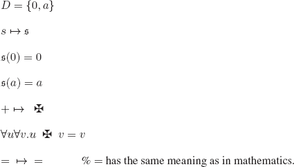
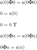
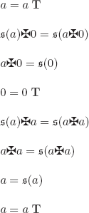
REMARK 12.1.– To avoid the (implicit) use of the axiom of choice, we can encode F : 0 T : 1 and define:

REMARK 12.2.– The argument used here is the same as the argument used to prove that there are uncountably many real numbers in the interval [0,1] (which entails that is uncountably infinite):

We assume that we can enumerate all real numbers between 0 and 1:

But the real number:

is not in this list (it is different from the first number at least at , from the second at least at ,... from the n^th at least at )

A contradiction; hence, the set of real numbers on [0, 1] is not denumerable.

EXERCISE 3.2.–

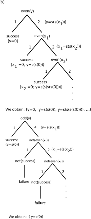
a) A truth function can always be represented by its graph, a its domain and range are finite.

The following example clearly shows how to proceed (it is trivial to transform this method into an algorithm).

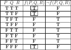
The dnf of f(P, Q, R) is:

The justification is very simple (properties of ∧ and ∨): every other combination of literals that appears in the dnf is equivalent to F (by inspection of the truth table).

The cnf of f(P, Q, R) is:

It is obtained because of the following equivalences:

and:

i.e. we take the conjunction of disjunctions for those f(P, Q, R) = F.

b) Use the equivalence and (a).

c) Use the equivalence and (a).

d) Use the equivalences and (a).

e) Use the equivalences and (c).

f) Use the equivalences and (b).

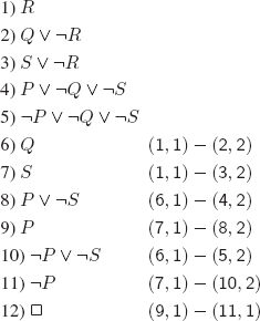
EXERCISE 3.3.– We provide a sufficient condition.

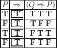
It is true if the only line with value F is the given one (see cnf, solution of exercise 3.2) or if the only line with value T is the one given (see dnf, solution of exercise 3.2).

EXERCISE 3.4.–

a)

EXERCISE 3.5.–

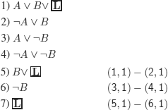
a)

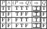
To know whether it is always F, we try to evaluate it to T:

to evaluate to T an implication, it suffices (this is not the only possibility) to fix its consequent to T.

It thus suffices to assign F to S and not bother with the truth values of the other propositional symbols to evaluate the given formula to T. It is not always F.

To know whether it is always T, we try to evaluate it to F:

to evaluate an implication to F, the only possibility is to have its first term evaluate to T and its second term evaluate to F.

We can evaluate it to F with the given assignments. It is not always T.

Conclusion: the given formula is neither contradictory nor a tautology.

b)

As mentioned above, to evaluate an implication to F, the only possibility is to evaluate its first term to T and its second term to F.

To evaluate the second term to F, the only possibility is:

and the only possible assignments are:

hence:

With these assignments, we try to evaluate the first term to T, the only possibility is:

With the only possible assignments for A, D, and E, we must assign C to T and F, which is impossible.

Conclusion: the given formula cannot be evaluated to F.

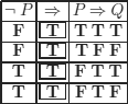
EXERCISE 3.6.– No, is not anti-symmetric (see definition 3.23):

Of course, for example:

But formula F is (syntactically) different from formula F ∨ F.

EXERCISE 3.7.–

a)

If we have P, any proposition implies P.

b)

If P is false, then P implies any proposition.

(a) and (b) are called paradoxes of material implication.

EXERCISE 3.8.– As is customary (in particular in mathematics), we convene that a reasoning is correct if and only if

REMARK 12.3.– This convention (definition) enables us to immediately propose two classes of reasonings that are trivially correct:

contradictory premises (inclusive) or tautological conclusion.

Before any translation, it is necessary to identify the synonyms and propositions that are negations of other propositions.

We propose:

S: Life has a meaning.

M: Life necessarily ends by death.

T: Life is sad.

C: Life is a cosmic joke.

A: Angst exists.

B: Life is beautiful.

B: Life is ugly (life is not beautiful).

M: Life goes on after death.

Most of the time we must make translation choices, but we will assume (this is not important, the important fact is to be aware of the difficulty of translation) that we all agree with the translation.

Once the translation has been made, we try (without forgetting to test the other possibilities if there is a failure) to find an interpretation that permits us to evaluate the conclusion to F and the premises to T.

If we succeed, the reasoning is incorrect and we have produced a counter example.

If we fail, the reasoning is correct.

Therefore, with this formalization, the reasoning is incorrect.

EXERCISE 3.9.–

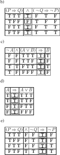
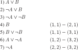
a)

Incorrect reasoning. Which is “natural”: in general, when the conclusion is independent from the premises, the reasoning is incorrect, except in the case of reasonings that are trivially correct (i.e. contradictory premises and/or tautological conclusion).

b)

As there is no other possible way of evaluating the conclusion to F and the premises to T, we conclude that the reasoning is correct.

If we had wanted to go from the premises to the conclusion (forward chaining), we would have done:

(only possibility), hence (contrapositive) (only possibility), hence (contrapositive) , hence (contrapositive) , i.e. ; thus, necessarily, for all the premises to be . We conclude that the reasoning is correct.

EXERCISE 3.10.–

a)

b)

c)

No, for example:

: cnf (a conjunct with three literals)

: dnf (three disjuncts, each with one literal)

d) No, it suffices to apply the distributivity of ∧ w.r.t. ∨

% Note the analogy with Cartesian product:

(i.e. 3 × 2 × 3 = 18 disjuncts)

e)

No.

Consider the wff:

The wffs G and H below:

Are two cnfs of F and they are different.

EXERCISE 3.11.-

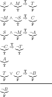
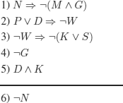
N: There is a unique norm to judge greatness in art.

M: M is a great artist.

G: G is a great artist.

P: P is considered as a great artist.

D: D is considered as a great artist.

W: W is a great artist.

K: K is a great artist.

S: S is a great artist.

The following formalization seems “natural”:

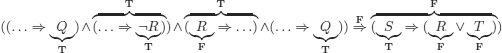
Forward chaining: we try to evaluate the set of premises to T (in every possible way) and verify that all models of this set are also models of the conclusion.

(→ shows the evaluation sequence)

in (4) G → F (only possibility) → in (5) D → T (only possibility); in (5) K → T (only possibility), hence in (3) W → T; hence, in (2) P ∨ D must be evaluated to F: impossible.

As there is no other choice to evaluate the premises to T, we conclude that the premises are contradictory, and hence the reasoning is trivially correct.

Backward chaining: if we can evaluate the conclusion to F and the set of premises to T, then we refute the reasoning.

(→ indicates the evaluation sequence)

in (6) (1) or (5) and (only possibility) (only possibility) must be evaluated to F: impossible. Hence (of course!) the same conclusion, meaning that we cannot refute the reasoning which is correct.

EXERCISE 3.12.–

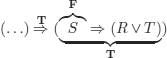
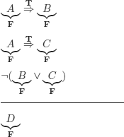
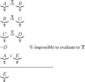
a) As we can evaluate the conclusion independently from the premises, we will be able to evaluate the conclusion to F and the premises to T. In general, the reasoning will therefore be incorrect.

Particular case: trivially correct reasonings (see exercise 3.9).

b) See proof of the following assertion exercise 3.30:

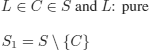
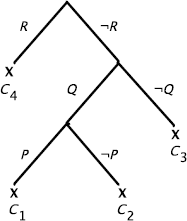
S: set of clauses, L C S, L pure

(*) S is contradictory iff S {C} is contradictory

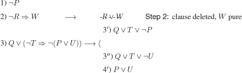
We shall prove that a reasoning is correct by proving that the set of premises together with the negation of the conclusion is contradictory. We can use property (*) for this verification.

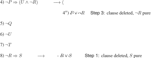
Example:

Step 1: we erase C₄ (T pure)

Step 2: we erase C₃ (U pure)

Step 3: we erase C₁ (R pure)

Step 4: we erase C₁P and Q pure)

S is thus equivalent to ; hence, non-contradictory (satisfiable). The reasoning from which S was generated was therefore incorrect.

EXERCISE 3.13.– We use the following propositional symbols:

C: Someone asked the house servant the question “…”.

R: The house servant answered.

E: Someone heard the house servant (the house servant was heard).

Q: Someone saw the house servant.

T: The house servant was busy polishing cutlery.

U: The house servant was here on the day of the crime.

The reasoning can be formalized as follows:

The reasoning is incorrect: the interpretation {Q}, i.e. Q evaluated to T and all other propositional symbols evaluated to F (see example 3.4) is a counter example.

Instead of verifying the correctness of the reasoning by using the same method as previously, we will do so in a way that is closer to the syntactic point of view of inference, similar to the inference rules used in mathematics, which will be treated in detail in section 3.3.

A major difference with the standard practice of mathematics is that we declare all the inference rules (elementary reasonings) that will be the only rules we will be allowed to use.

Inference rules:

and (intro):

and (lelim):

and (relim):

or (intro):

contrap:

disj. syl.:

abd: % Warning: abd is not a correct rule (see definition 3.12). It is used to discover premises in abduction (see section 8.3).

a) A trivial possibility: add U to the premises.

Other possibilities (closer to the intuitive notion of an explanation)

Forward chaining:

a1) We add Q and we deduce:

Other possibility:

a2) We add and (a1), we obtain U.

Backward chaining:

a3) We add Q and we obtain U as above.

b) There are infinitely many solutions (redundant intermediate chains that can be removed).

c) No: either the added premises are in contradiction with the existing premises, in which case the reasoning is trivially correct, or we carry out the same proof, as we did before the addition of the premises.

The key remark here is that a model of a set of formulas is a model of all the formulas in the set.

Assume and:

can be any formula, in particular, the “strange” case where (because it is impossible to evaluate the premises to T and C to F).

(*) means that there exists an interpretation that is a model of {P₁, P₂, …, P_n, Q} and a counter-model of C.

But a model of {P₁, P₂, …, P_n, Q} is also (by definition) a model of {P₁, P₂, …, P_n}, and every model of {P₁, P₂, …, P_n} is a model of C; hence, (*) is impossible.

REMARK 12.4.– In the formal system (see definition 3.9) whose inference rules are those above, it is possible to prove the ex falso quodlibet principle: “from a contradiction we can deduce any conclusion” (see also exercise 3.26).

EXERCISE 3.14.– only if)

Trivial. By definition:

A B means: every model of A is a model of B. This means that A B cannot be evaluated to F, i.e.:

if

|= A B means that it is impossible to have interpretations that evaluate A to T and B to F, in other words:

EXERCISE 3.15.–

a) Particular case of exercise 3.14.

b)

only if)

All models of are models of C (definition of ), hence, are counter-models of is evaluated to F, then so is is evaluated to T, then C is evaluated to F, and so is . conclusion: is unsatisfiable.

if)

It suffices to restrict ourselves to the interpretations of that are models of .

If is a model of , then by definition of unsatisfiability, , hence therefore, .

EXERCISE 3.16.–

Answer: (b)

We prove so by reductio ad absurdum.

Assume A B, hence:

(definition of )

but (hypothesis)

thus (transitivity of )

contradiction, therefore:

EXERCISE 3.17.–

True.

The reasonings will be of the following form.

Premises:

conclusion:

where for and .

Indeed, a S is minimally unsatisfiable, is satisfiable and every model of S₁ must be a counter-model of f₁ (a S is unsatisfiable), i.e.:

REMARK 12.5.– This property can be viewed as a generalization of the proof technique that consists in proving the contrapositive.

If we have proved

by proving:

unsat,

then we have also proved that

(if C is T, then must be F, otherwise the set would be satisfiable):

i.e.:

or, in other words:

EXERCISE 3.18.–

a) The ideas and remarks that will enable us to construct the interpolant are the following:

1) Each line¹ of the truth table of a formula is an interpretation of (the truth table enumerates all the interpretations of ). We shall mention interpretation with the same meaning as line in the truth table.

2) The interpretations of interpolant to be constructed will, in general, be partial interpretations of {,} (except in the case in which Propset () = Propset()).

3) Key remark. Given an interpretation of , does there exist an interpretation of {, }, that is an extension of and such that:

As, by hypothesis, , i.e. every interpretation satisfying also satisfies , such an interpretation I does not exist.

4) We want hence, if line 1 of the truth table of evaluates to T and l contains line l_C of the truth table of , then we will evaluate line l_C of to T.

5) We want hence, if line l of the truth table of evaluates to F and contains line l_C of the truth table of C, then we will evaluate line l_C of C to F.

6) There cannot be any conflict between steps (4) and (5) (see remark 3).

7) For the cases in which line l evaluates to F (respectively, to T), we can arbitrarily choose to assign values T or F to line l_C of , which means that, in general, there are several possible interpolants (2ⁿ, where n is the number of lines from which we can choose).

8) Points (1)-(7) above are about the truth table of . The method described in exercise 3.2 enables us to construct the dnf (or cnf) of .

(1) -(8) above give the algorithm to construct and prove its correctness at the same time.

b) Propset () = Propset() = Propset() = {A, B, C}

By applying the method of exercise 3.2, we obtain the 8(=2³) possible interpolants:

c) Propset() = {A, B, C}; Propset() = {B, C, D}; Propset() = {B, C}

EXERCISE 3.19.–

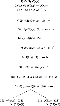
Tree 1

Tree 2

EXERCISE 3.20.–

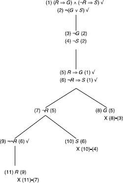
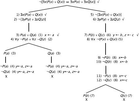
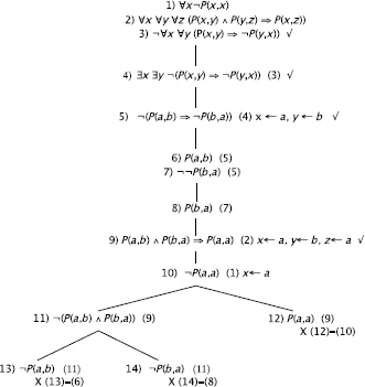
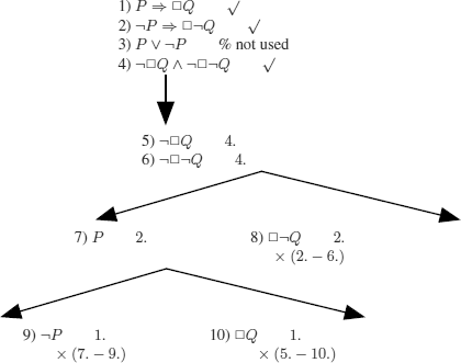
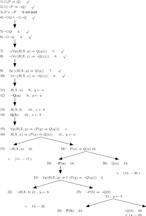
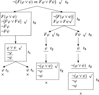
a)

Correct reasoning

The }’s, the 's, and the arrows correspond to the operations:

of the algorithm SEMANTIC TABLEAUX (PL).

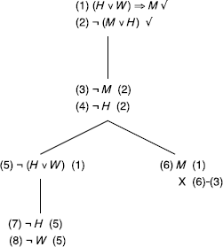
b)

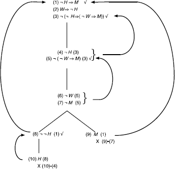
Correct reasoning

c)

Incorrect reasoning, counter example: {¬H, ¬M,¬W}

d)

Incorrect reasoning, counter examples: {¬A, ¬B,C}, {¬B,C}, and {A, ¬B,C}

e)

Incorrect reasoning, counter examples: {P, ¬Q,R, T } and {¬P,Q, ¬S, ¬T }

f)

Incorrect reasoning, counter examples: {P,Q,R, ¬S}, {P,Q,R}, and {P,Q,R, S}

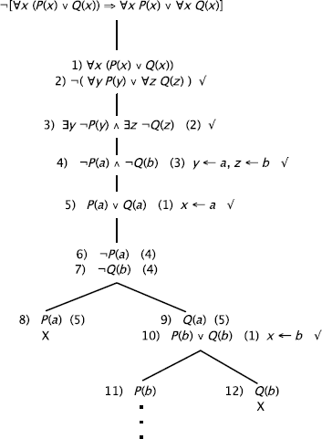
g)

Thus, the initial formula is valid.

EXERCISE 3.21.–

a)

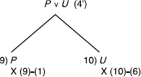
The set of formulas is satisfiable, with models {¬P,R, S, ¬Q} and {Q, P, ¬R, ¬S}

b)

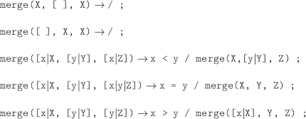
Although this is not necessary at all, sometimes, a preprocessing can enable us to simplify the problem under consideration. We illustrate this by applying the purity principle, i.e. the removal, in a set of clauses, of those clauses containing pure literals, since such an operation preserves the (un)satisfiability of the set (see exercise 3.30).

We must thus transform S₂ into an equivalent set of clauses.

The set of formulas is unsatisfiable.

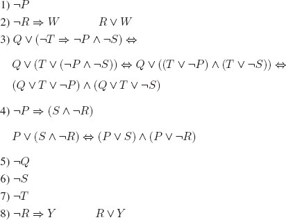
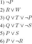
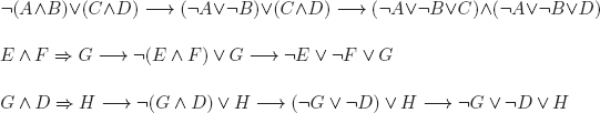
EXERCISE 3.22.– We give two reasons.

1) If they were defined as functions:

– they would either be partial functions, for example:

– or we use a trick:

2) We would like to have, for example:

but also:

This inference rule is clearly not a function, as it gives two distinct values for the same argument.

In general, it is impossible to consider inference rules as functions without any problem arising.

EXERCISE 3.23.– We want to prove:

If , then

PROOF.– By definition, there exists a deduction of starting from Γ

if we add A to the hypotheses, we obtain B by MP on A and , i.e.

EXERCISE 3.24.–

a) MP is correct: every model of A and is necessarily a model of B (otherwise B would be F, by definition of ).

We can easily verify that all the axiom schemas are tautologies (valid wffs). Hence, by definition of a valid wff and by induction on the number of steps in the proof, we conclude that every theorem of S₁ is a valid wff.

b) Assume that there exists such that A and .

As shown in (a) above, every theorem of S₁ is a valid wff. The negation of a valid wff is not a valid wff, hence it is not a theorem (contrapositive).

Therefore, such a wff A cannot exist.

c) Truth tables (semantic tableaux, the Davis and Putnam method, etc.) permit us to decide whether a wff is valid or not. As we admitted that S₁ is adequate, we have a decision procedure for S₁.

REMARK 12.6.– The soundness proved in (a) is not sufficient to prove (c). Indeed, the former says: if not valid then not a theorem. But if adequacy (completeness) is not guaranteed and the wff under consideration is valid, then we cannot be sure that it is a theorem of S₁ (it could be a valid wff that is not captured as a theorem by the formal system).

EXERCISE 3.25.–

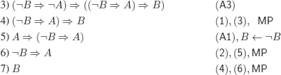
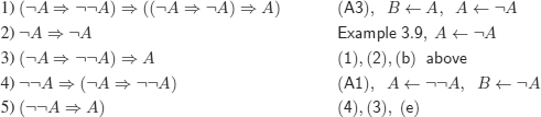
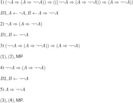
a)

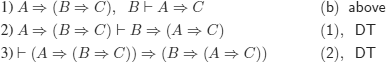
We can always use a theorem that was already proved. The justification is simple: we copy its proof at the beginning of the proof that uses it. The proof thus obtained respects the definition of a proof.

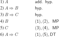
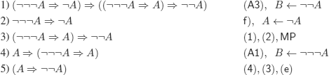
b) We give two deductions, one of which uses the deduction (meta-) theorem (abbreviated as DT).

i) Without using the DT

ii) Using the DT

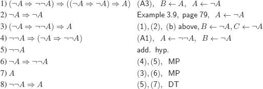
c)

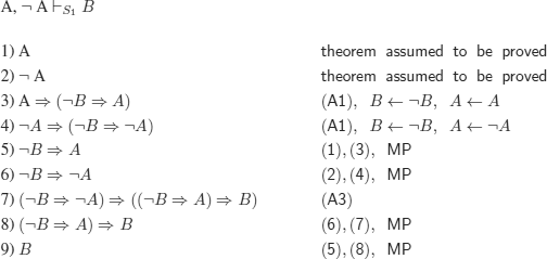
d)

Warning: though tempting, the contrapositive cannot be used (it has not yet been proved that it is a theorem of S₁).

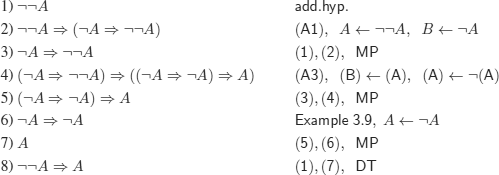
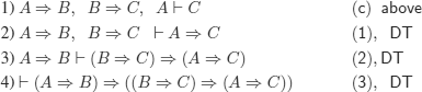
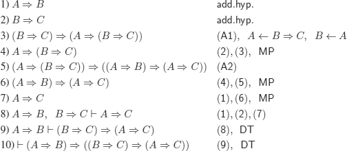
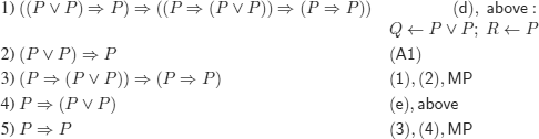
e) We give two deductions, one of which uses the deduction (meta-)theorem (abbreviated as DT).

i) Without using the DT

ii) Using the DT

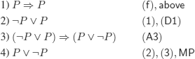
f)

Other proof:

Another one:

g)

h)

Other deduction

i)

EXERCISE 3.26.–

We must prove:

S₁ is consistent w.r.t. negation if S₁ is absolutely consistent.

only if

We prove the contrapositive. We assume that , i.e. that very wff is a theorem. in particular:

hence, S₁ is not consistent w.r.t. negation.

if

We prove the contrapositive. We thus assume that there exists A L such that:

We first prove:

Hence, as B can be replaced by any wff, we conclude that every wff is a theorem.

EXERCISE 3.27.–

a)

b)

c)

d)

e)

f)

g)

h)

EXERCISE 3.28.–

a) Yes, by verifying that:

(B2) is the same axiom schema as (A1) (in S₁);

(B4) is the same axiom schema as (A2) (in S₁);

and by taking remark 3.24 into account.

b)

EXERCISE 3.29.–

a) We will say that two formal systems with the same language (or with languages that can be formally translated from one to the other) are equivalent iff they have the same set of theorems.

b) consider:

– the formal system

– a subset of axioms

– the formal system

is independent iff x, for all x χ.

For example, the formal system (see (c) below), which differs from S₁ only in the set of axioms, is not independent.

c)

(as see example 3.9)

d) (analogous to (b))

Consider:

– the formal system

– a subset of inference rules

– the formal system

is independent iff there exists A and s_i, such that s_j A.

e) Find (it is not guaranteed that this will succeed) a property P such that:

1) the elements of /χ have property P;

2) the rules of R preserve property P;

3) the elements of χ do not have property P.

REMARK 12.7.– This technique was used to prove the independence of the famous “parallel postulate”, which led to non-Euclidean geometry.

Interpretations that are models of the other axioms of Euclidean geometry and counter-models of the parallel postulate have been found.

EXERCISE 3.30.–

(R-0)

Without loss of generality, we assume that S contains a unique tautological clause T.

Let S₁ = S {T}

S is unsatisfiable iff S₁ is satisfiable.

if

We prove the contrapositive:

S satisfiable.

By definition, every subset of a satisfiable set is satisfiable; hence, S₁ is satisfiable.

only if

We prove the contrapositive:

S₁ is sat, with model, say, M.

As T is satisfied by every interpretation, it must be satisfied by M; hence, S is sat.

(R-1a) Trivial. No interpretation can make both L and T.

(R-1b) (To simplify the notation, we assume there is only one unit clause {L} and only one clause of the form . Of course, the reasoning can be repeated.

S₁ = ((S {L}) ({L^c} ∪ α)) ∪ {α}

S unsat iff S₁ unsat.

only if

We prove the contrapositive.

Assume S₁ is sat, let M₁ be a model of S₁. Without loss of generality, we can assume (otherwise, it can be removed from M₁ without any consequence). There exists such that (all the clauses in S₁ must be evaluated to T).

is a model of S. Therefore, S is sat.

if

We prove the contrapositive:

Assume S is sat, let M be a model of S. Necessarily, (and therefore ). There exists K α such that thus, S₁ is sat.

(R2)

We assume without loss of generality that there is a unique pure literal:

S is unsat iff S₁ is unsat.

only if

We prove the contrapositive.

Assume S₁ is sat, let M₁ be a model of S₁, (as L is pure).

is a model of S, which is therefore sat.

if

We prove the contrapositive.

S sat and . cannot be unsat because every model of S is a model of all the clauses in S. Thus, S₁ is sat.

This rule is known as the purity principle.

(R3)

S unsat iff (S₁ unsat and S₂ unsat)

only if

We prove the contrapositive.

S₁ sat or S₂ sat.

Without loss of generality, we assume that S₁ is sat (we do not consider the case in which S₂ is sat, as the proof is similar).

Let M₁ be a model of and there exists .

is a model of S. Hence S is sat.

if

We assume without loss of generality that there is only one clause containing L (say, the clause ) and only one clause containing L^c (say ).

We prove the contrapositive.

S is satisfiable, let M be a model of S. Assume ; hence, . As M is a model of all the clauses in S, there exists a such that hence, S₂ is sat, and S₁ is sat or S₂ is sat. Same reasoning if .

If and , there exists , such that Hence S₁ sat and S₂ sat.

(R4)

S unsat iff S₁ unsat

if

We prove the contrapositive.

S sat. As is sat.

only if

We prove the contrapositive.

S₁ sat, let M₁ be a model of S₁. Of course, M₁ is a model of ; hence (definition of a clause), M₁ is also a model of . Therefore, S is sat.

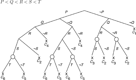
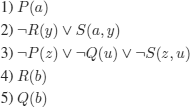
EXERCISE 3.31.– The answer is yes, as shown by the application of the algorithm with the strategy below.

In example 3.13, we implicitly applied the strategy “find a model as soon as possible”.

We now apply the strategy “try to find as many models as possible” (actually, in this particular case, we find all of them).

We thus found the following six models:

EXERCISE 3.32.–

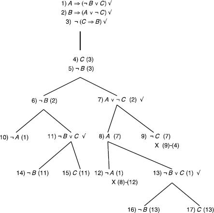
a) We take the following (arbitrary) order for the basic formulas:

O: inference nodes

b)

The interpretation that we can give of the inference nodes is as follows:

The interpretations denoted by the two branches going through an inference node falsify the clauses and ( and : disjunctions of literals). By definition of a clause, the interpretation denoted by the branch that finishes by an inference node falsifies all the literals of and all the literals of . It therefore falsifies the resolvent of C_i and C_j (see definition 3.15).

c)

EXERCISE 3.33.–

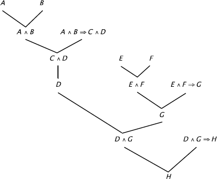
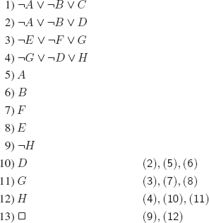
EXERCISE 3.34.– We must prove:

If S is unsat, then (see section 3.7)

We give two proofs of this result.

PROOF 1.– We prove the result by induction on the number of positive literals in S.

1)

Since S is unsatisfiable, S is necessarily of the form:

S = {L, L^c} hence, by applying the resolution rule once we obtain:

ii) n > 1

The idea is to apply a transformation that preserves the unsatisfiability, and strictly decreases the number of literals (to apply the induction hypothesis).

Assume S contains n + 1 literals.

Choose a literal that is not pure.

Consider the sets of clauses:

It was proved (see exercise 3.30) that:

S is unsat 1 iff S₁ is unsat and S₂ is unsat.

By the induction hypothesis, % S₁ contains at most n literals.

There are two cases to consider (the second case itself leads to two cases):

a) the clauses do not occur in the refutation of S₁.

The clauses that occur in the refutation are also in S, hence:

.

b1) the clauses C{L} occur in the refutation of S₁.

In this case, , as can be proved by generalizing the following example.

If we add a pure literal to the first clause:

b2) by repeating exactly the same reasoning for S₂ with L^c instead of L, we conclude that:

Now for S (containing n + 1 literals) we have:

hence, by applying once the resolution rule, we obtain: .

PROOF 2.– We give another proof by using theorem 3.2, and the results of exercise 3.32 (b).

By theorem 3.2, if S is unsat then there exists a closed semantic tree T for S.

First note that in a closed semantic tree, there are always inference nodes, otherwise all clauses would be positive (respectively, negative), and by applying the purity principle (see exercise 3.30), we would obtain an empty set equivalent to S, which would thus be satisfiable.

By eliminating all failure nodes from T, we obtain a closed tree T' (with strictly less nodes than T), corresponding to the set of clauses:

We repeat the reasoning, but this time on S'.

As we are starting with a finite closed tree and at each step we obtain strictly smaller closed trees, we necessarily obtain a finite tree with ¬L and L (of course L denotes an arbitrary literal) as left and right branches, respectively, and the corresponding inference node is .

EXERCISE 3.35.– We must show:

We first prove that if S is unsat then (see the definition of operator (definition 3.16)) is unsat.

The proof is trivial: every superset of an unsat set is unsat.

As we have proved the completeness of resolution for refutation, it suffices to apply rule R-0 of the Davis and Putnam method to Rⁿ(S) (unsatisfiable set of clauses) for every n ≥ 1.

EXERCISE 3.36.– As resolution is complete for refutation, if S is unsat then will be derived after a finite number of steps.

Given a set of clauses S, the problem is to decide whether S is sat or unsat. As S contains a finite number of literals and the application of R_c does not add any new literal, after a finite number of steps, we either generate or we do not generate any new clause. In the latter case, we say we have saturated the set of clauses.

When the set of consequences of S has been saturated, the refutational completeness of S enables us to conclude that S is satisfiable.

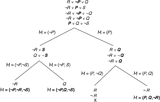
An application example of this decision procedure is the detection of the satisfiability of the set of clauses (1), (2), (3) below:

EXERCISE 3.37.–

a)

b)

c)

There is no way of obtaining different clauses; hence, S is satisfiable.

d)

We give the clausal translation of each formula:

We prove that the set of clauses is unsatisfiable:

e)

i) if we did not know the resolution rule, we would probably give a proof similar to the following:

ii) By applying the resolution rule. We first translate into clausal form:

By negating the conclusion, we obtain the set of clauses 1-9 below and a refutation using resolution.

REMARK 12.8.– In (10), (11), and (12) we used the hyperresolution rule (we “compress” several resolution steps into only one).

f) We must consider the set of clauses 1-8 below, obtain all possible resolvents and reach saturation without generating .

EXERCISE 3.38.– Not necessarily, the set of clauses:

does not contain any pure literal, but contains proper subsets that are unsatisfiable.

EXERCISE 3.39.–

a)

b) No. Take for example the unsatisfiable set of clauses:

We cannot deduce using an input strategy, because the set does not contain any unit clause. Indeed, can only be generated by two complementary unit clauses, one of which must belong to S (this is required by the input strategy).

EXERCISE 3.40.– No. Take the same unsatisfiable set as in exercise 3.39:

We cannot apply the resolution rule with a unit strategy.

EXERCISE 3.41.– Every interpretation I of S can be represented (see example 3.4, point 2.) by:

, where and (see definition 3.8).

As S contains all the clauses of length n that can be formed with n propositional symbols, S contains a clause:

In other words, if L_i is in I then ¬L_i is in C_j and if ¬L_i is in I then L_i is in C_j.

C_j is falsified by I; hence, S is falsified by I.

This reasoning holds for all interpretations of S, which is therefore unsatisfiable.

EXERCISE 3.42.–

a) Every interpretation I of S contains (at least) p literals L₁, L₂,... L_p with the same sign.

By construction, S contains a clause , which will of course be evaluated to F in I.

Therefore, S is unsatisfiable.

b) No.

Take as a counter example n = 2 (say {A, B}); hence, p = 2

, which is satisfiable

(We could have chosen n = 4, n = 6, …)

The explanation of the counter examples is that there could be, with the new hypothesis on p, interpretations containing only q literals of the same sign, with q < p.

EXERCISE 3.43.–

a)

We consider the propositions meaning .

We give the set of clauses specifying that such an injective function exists. This set must therefore be unsatisfiable.

The clauses specifying all possible images of the elements of the domain of cardinality n(S_n):

The clauses specifying that the function is injective will be of the form:

We will thus have:

n × (n - 1) propositional symbols

n clauses of length n - 1 (*)

n × (n - 1)² ÷ 2 clauses of length 2 (**)

The general case:

b) S₃ (clauses 1-9):

REMARK 12.9.– It is possible to prove that the minimal number of clauses necessary to refute the set of clauses specifying the pigeonhole Sn is:

For S₃, the shortest refutation then contains 2 × 5 × 1 = 10 clauses.

The pigeonhole was used to prove that the resolution method is exponential, i.e. that there exists at least a set of clauses for which the shortest refutation is exponential in the number of clauses.

REMARK 12.10.– We sometimes specify the pigeonhole problem by translating: “If we define a function from n + 1 objects onto n objects then there exists (at least) two objects of the domain with the same image”, which translates into the tautological schema:

EXERCISE 3.44.–

No. We give two proofs of this result.

a)

As all clauses are of the form:

with:

P_i: positive literal;

N_j: negative literal;

the interpretations I = {P_i} and J = {N_j} are models of the set of clauses that can therefore not be unsatisfiable.

b)

As the resolution is complete for refutation, we can assume without loss of generality that we are trying to detect the unsatisfiability of the set of clauses using the resolution rule.

The set does not contain any unit clause. indeed, as a unit clause contains only one literal and as a literal is either positive or negative, if the set contained a unit clause, the hypotheses would be violated.

Thus, all clauses are of the form:

Without loss of generality, we reason on clauses of length 2. The application of the resolution rule to

produces a clause of the form:

Therefore, we can never obtain the complementary unit clauses that are necessary to obtain .

The required corollary is trivial to obtain. The question is whether a set of clauses containing a positive clause (respectively, negative clause) but no negative clause (respectively, positive clause) can be unsatisfiable. The answer is no. In the first case, the interpretation

is a model. In the second case, the interpretation

is a model.

Hence the conclusion.

EXERCISE 3.45.– We use the propositional symbol:

: country i is colored with color j.

Each country is colored with exactly one color:

for

By transformation into clausal form (simplifying the clauses containing tautologies and applying the subsumption rule), we obtain the equivalent specification:

(Sch1) for

(Sch1) could also have been obtained by translating: “country i must be colored with a color (first conjunct) and we cannot color it with more than one color (three other conjuncts)”.

The complexity of the specification of these clauses is less than 3 × N, or in other words, O(N).

Two neighboring countries cannot be colored the same way:

(Sch2) for all neighboring countries i, j:

Every country has at most N - 1 neighbors, hence there are less than N² clauses similar to the clause above. Hence, the complexity of the specification of this second part is O(N²).

The global complexity is thus O(N²).

REMARK 12.11.– In the coloring problem of example 9.19, the solution was obtained using a specification with constraints.

We could apply the formula schemata (Sch1) and (Sch2) above to specify the same map and the method of semantic tableaux (see section 3.6) to find all the models (i.e. the solutions to the problem). Of course, the solutions must be the same. It could be interesting to compare both approaches (one numerical, the other logical).

EXERCISE 3.46.–

a)

We assume that the models are represented by the set of propositional symbols that are evaluated to T in the models (form 3 in example 3.4).

Of course, the theorem does not depend on the adopted representation of models.

We note:

PROOF.– To derive a contradiction, we assume:

, hence, for at least one clause :

There are two cases to consider (depending on the different forms of Horn clauses, see definition 3.21).

i) (m = 0 corresponds to a unit positive clause)

To evaluate a clause to F, it is necessary to evaluate all of its literals to F (see definition 3.14), i.e.:

hence, by definition of an intersection, there exists such that:

but then M_k is not a model of H (as it falsifies one of its clauses: C_j). Contradiction.

ii)

To evaluate C_j to F:

hence, by definition of an intersection, for all

but then the M_k’s are not models of H (as they falsify one of its clauses: C_j).

Contradiction.

b) No. Take

and

then , which is not a model of H.

EXERCISE 4.1.–

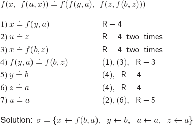
a)

R-4 on = yields:

R-4 on = yields:

R-3 on = yields:

R-4 on = yields:

R-5 on = yields:

There are no rules that can be applied, we halt.

Solution:

b)

c)

d)

Yes, it is always necessary. Consider the equation:

Clearly,

If we do not apply the cycle rule, we have:

i.e.:

which is an infinite term.

A sufficient condition to be able to deal without the cycle rule is:

and (t₁ or t₂) linear (a term t is linear iff all of its variables occurs at most once in t).

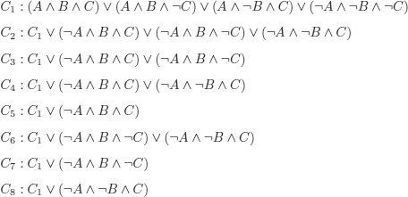
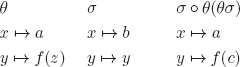
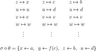
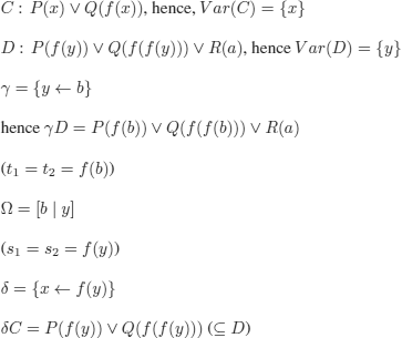
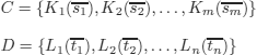
EXERCISE 4.2.– The possibilities of identification of the (sub)formulas corresponding to A, B, C in CD are:

1)

2)

3)

4)

There remains to compute three mgus and three direct consequences in the case in which the mgus exist, cases (3) and (4) are of course identical.

We note that the only useful direct consequence is the first consequence (the others are wffs that coincide with the premises).

EXERCISE 4.4.–

– To be able to compare the rules and verify what is asked, we need to choose a same language to represent the three rules. We choose the language of clauses.

– To be able to apply the UNIFICATION algorithm (as well as the modified UNIFICATION), we consider connectives as functional symbols.

– Terms are formed from functional symbols of fixed arities and , which explains why we use , which ordinarily denotes the empty string of symbols (i.e. the disjunction without any disjunct) in the terms representing the inference rules.

– this is a matching problem; hence, we use for R symbols that ordinarily denote variables.

– A, B, X denote literals; denote clauses.

The solution of equation:

found by UNIFICATION is:

The solution of equation:

found by modified UNIFICATION is:

EXERCISE 5.1.–

a)

b)

Model:

Counter-model:

Only change

c)

d)

e)

f)

g)

Model:

Counter-model:

Change D =

h) No.

Take, for example:

i)

REMARK 12.12.– One characteristic of the equality relation is that it can be applied to (and have a meaning in) any domain of discourse.

j)

Counter-model with:

(take, for example, x = 3,y = 4 and z = 5)

k)

This formula does not have any finite model. It is a total, transitive and irreflexive relation. See also example 9.33.

We prove this by reductio ad absurdum. Assume it admits a finite model of domain:

also,

also,

but as D is finite (and of cardinality n), after at most n – 1 steps, we must produce (by transitivity) with q = r (because a_q is related to one of the a_is in D, which will be reached sooner or later).

This is contradictory because is irreflexive.

Therefore, this formula has no finite model.

1)

We can give infinitely many models for this formula by choosing:

For relation A, we choose any relation such that each element is in relation with exactly two other elements.

For example:

Which can be represented by the following graph:

We obtain a counter-model by adding at least a couple (an edge) to the relation (to the graph representing the relation), for example:

m)

with

meaning that for each x, the corresponding y and z are y = 2 × x and z = 2 × x + 1

The values of y and z can of course be interchanged.

m₂)

This formula has no finite model. We assume a finite domain exists, with domain of discourse:

and derive a contradiction. By definition of a model, for all k D there exists i, j, i ≠ j such that:

Since is not injective and D is finite:

To satisfy the formula (see definition 5.6), all elements of:

domain () range () must have antecedents in D = domain (), but these potential antecedents already have values in the range ().

It is impossible (definition of a function) to assign other values to them. The finite model hypothesis leads to a contradiction.

Therefore, this formula does not have any finite model.

A way of visualizing this reasoning is to draw the graph of function . The elements marked with correspond to those that cannot be reached in a finite domain of discourse.

n) No.

See example 9.31, the definition of a finite set:

The set E is finite iff all injective functions E → E are also onto. See also example 9.32.

o)

Consider the interpretation :

We verify that is a model of (1) and (2) and a counter-model of (3):

1)

2)

3)

EXERCISE 5.2.– We use the same idea as in example 5.13, i.e. we consider a formula of the form and we focus on the case in which n ≥ 2. The problem is thus to find an adequate wff .

There exist sets of arbitrary finite cardinalities (think for example of the finite subsets of ). To specify this, we must say that:

1) there exist n objects;

2) these objects are all different (so that the set is indeed of cardinality n).

1) translates into:

Meaning that there are n objects with some property P; this is the usual method of defining sets.

2) To specify that they are different, it suffices to state that if an object x_i has a property, then another object x_j (i ≠ j) does not have it. Thus, it cannot be the same object.

The only remaining problem is how to choose (name) these properties. If we choose P (the same as the one used to define the set), the wff would be contradictory and the implication would be trivially T; similarly, if we choose only one property distinct from P (simple to verify with n = 2 and n = 3).

The solution is simple: it suffices to choose distinct properties, i.e.:

with (i.e. all possible combinations of two objects among n).

There remains to prove (by induction) that the proposed formula is n-valid for all n (n ≥ 2).

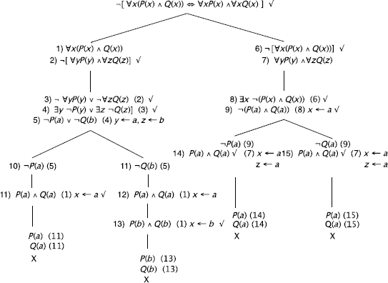
– n = 2. It is very simple to verify (for example, using the method of semantic tableaux) that the formula is n-valid (i.e. 2-valid).

– n = N +1

We must add together with the formulas:

In branch (1) of the tree, there would be

together with P(x₁), P(x₂), …, P(x_n+1), i.e. n + 2 potential constants. To work in universes of cardinality n +1 and using the induction hypothesis, we shall let x_i = x_n+1 (1 ≤ i ≤ n). The branches of depth N + i (1 ≤ i ≤ n) will all contain either Q_N+i(x_i) and ¬Q_N+i(x_i) or ¬Q_N+i(x_i) and Q_N+i(x_i) (of course, this is done under the assumption, which does not incur any loss of generality, that the tree was developed in increasing order of the variable indices) and whatever the chosen instantiation, will all be closed.

The formulas for (unbounded) arbitrary cardinalities can be obtained using the following schema:

thus using:

unary predicates Q_l

with:

EXERCISE 5.3.– a)

b)

c)

d)

e)

The method continues with , …the tree will not be closed (this will not be detected by the method).

REMARK 12.13.– If we had not renamed the variables, i.e. if instead of (3) we had written then we could have “proved the validity” of the given formula.

f)

g)

h)

REMARK 12.14.– The replacement y ← d that was used to obtain formula 13 is correct as constant d was not used to replace any other existentially quantified variable.

i)

REMARK 12.15.– Here we used the fact that the semantics of FOL requires that the functions assigned to the functional symbols be total functions. Indeed, otherwise, we would not be able to replace variables by (for example) f (a). Furthermore, if (for example) f (a) is not defined then Q(f (a)) and ¬Q(f (a)) would not be contradictory ( and ¬ is not contradictory).

j) (See also section 8.3.)

By examining the tree, we notice that we could Close the tree by adding the formula .

or

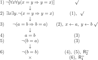
k1) To verify the validity of the formula, we negate it.

k2) To try to construct a model of the formula, we do not negate it.

We can extract the following models from the finite open branches:

We can extract the following model from the infinite branch:

1)

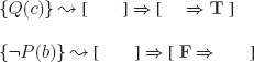
EXERCISE 5.4.– The tableau corresponding to the given reasoning:

It is Clear that if:

– the cardinality of the domain of discourse is 1, i.e. a = b = c, then we obtain a closed tree (P(a), ¬P(c));

– similarly if the cardinality of the domain of discourse is 2, i.e. a = b (S(b), ¬S(a)) or a = c (P(a), ¬P(c)) or b = c (R(b), ¬R(c));

However, if the cardinality of the domain of discourse is 3, i.e. a ≠ b and a ≠ c and b ≠ c, we obtain the following model from the set of formulas (1), (2), (3), (4)".:

(P(b), Q(b), Q(c), R(a) can belong to or not)

It is very simple to verify that this is a counter example of the reasoning on a domain of discourse of cardinality 3. By construction, is a model of the premises. About the conclusion:

– if x = a, then in we have S(a): F and Q(a): T ;

– if x = b, then we have S(b): T and Q(b): F ;

hence, in all cases, the conclusion is evaluated to F.

EXERCISE 5.5.–

EXERCISE 5.6.–

i.e.:

i.e.:

i.e.:

Note that is also a model of , as is a set of Horn clauses (see exercise 3.46).

EXERCISE 5.7.– We are here in the case of example 5.16, wherein we had to apply the method of semantic tableaux to what we called “generic formulae”.

Without loss of generality and for the sake of clarity of the proof, we write the binary resolution rule under the form:

To prove that the resolvent is a logical consequence of the parent clauses, we construct the tableau below.

It should be clear that we transformed the disjunctions of literals into binary trees (which is required by our formalization of semantic tableaux) and that:

The use of substitution O (instead of simply ) can be explained by the fact that possibly, . In this case

Similarly for the are variables of the parent clauses) (instead of a, any other closed term could be used). γ, which can also take into account the possible renamings of the variables of the resolvent, is thus used exclusively to close branches because of contradictions between closed literals (i.e. containing only closed terms), thus ensuring that the rules of the method of semantic tableaux are applied to formulas that are propositional (up to the syntax).

These are constant instances corresponding to the literals of the parent clauses whose variables are quantified universally (and as usual we chose the instances to be able to close the branches).

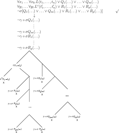
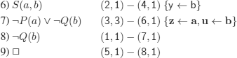
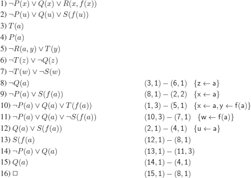
EXERCISE 5.8.– First we must transform the premises and the negation of the conclusion into clausal form (the labels on → refer to the rules used in the proof of theorem 5.3).

We rename the variables to avoid any confusion:

Negation of the conclusion:

% i.e. two clauses

To prove that the reasoning is correct, we must refute clauses 1. to 5. below:

Exercise 5.9.–

by replacing:

if we had asked the question

instead of we would have generated (see exercise 3.34):

Answer (h(g(c, b, f (a, c, d))))

which translates, in accordance with the interpretation that we gave to the function symbols (in particular to the constants) into: the monkey climbs on the chair after having walked from a to c starting from d, and carried the chair from c to b.

EXERCISE 5.10.–

a)

b)

REMARK 12.16.– We systematically rename the variables of the resolvents.

These are sets of clauses that belong to a decidable fragment of FOL (the clauses do not contain any functional symbol). After a while, no new clause is generated (up to a renaming of the variables) and since is not generated, we conclude that the set of clauses (1) to (5) is satisfiable.

EXERCISE 5.11.–

To apply the resolution rule, we must transform into clausal form: from , after Skolemization we obtain .

For the conclusion, :

negation → Skolemization:

The set of clauses to consider:

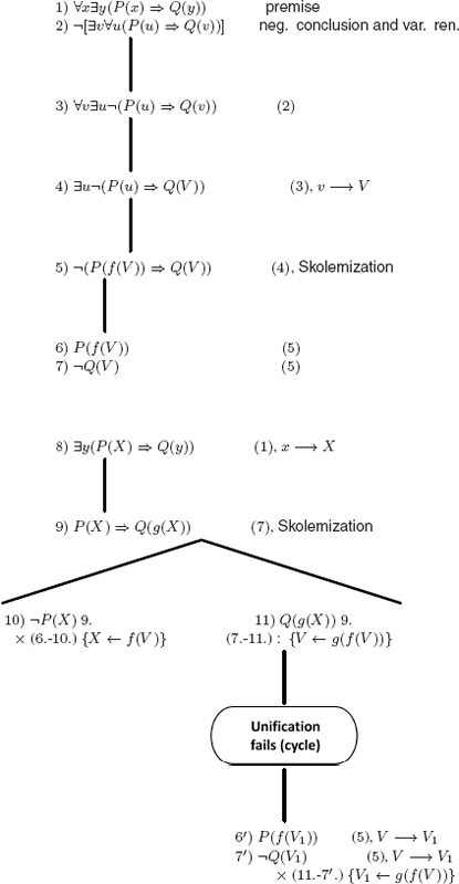
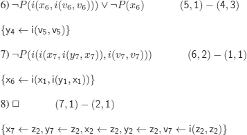
The resolution rule cannot be applied (the unification algorithm fails with c1ash), cannot be obtained: the answer is therefore no.

EXERCISE 5.12.–

i) This exercise shows how to encode the axioms and the inference rule of S₁ in clausal form and prove theorems using the resolution rule.

We write (A1), (A2), and (A3) in clausal form. The connectives and are written:

i(x,y): x y

n(x): x

1) P(i(x,i(y,x)))

2) P(i(i(x, i(y, z)), i(i(x, y), i(x, z))))

3) P(i(i(n(y), n(x)), i(i(n(y), x), y)))

The axioms are provable.

To translate MP, we say: If x is provable and is provable, then y is provable:

4) P(i(x,y)) ∨ (x) ∨ P(y)

We ask the question ^? A A (see example 3.9). To better recall that A is a (meta) variable that denotes an arbitrary wff, we write ^? v v (v denotes a variable).

To show that v v is provable in S₁ (encoded P(i(v, v))), we must generate, applying the resolution rule on 1–4 and:

As usual, we identify the variables in each clause with the corresponding index and rename the variables of the resolvents. We use a linear strategy.

ii)

We proceed by reductio ad absurdum. We assume that

A A is not provable (5)

This implies that A is not provable, or that A (B B) is not provable (6);

and that, in turn, (A (B A)) (C C) is not provable (7)

As A, B, C are meta-variables (i.e. variables that can be replaced by arbitrary wffs), to avoid any confusion, we shall name them X, Y, Z respectively, so that

(X (Y X)) (Z Z) is not provable.

One instance is (with X ← C, Y ← C, Z ← C C):

(*) is also an instance of (A2)

But this is a contradiction, as all the instances of an axiom are (by definition of a proof) provable.

EXERCISE 6.1.-

a)

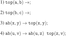
ab(c, a); % the question

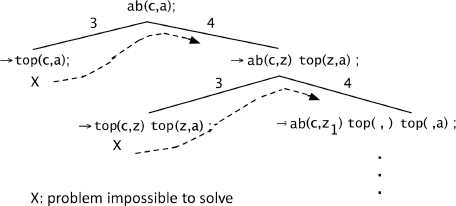
The execution does not halt.

If we consider the clause (**) instead of (*) :

1) top(a, b) →;

2) top(b, c) →;

3) ab(x, y) → top(x, y);

4) ab(u, v) → top(u, z) ab(z, v);

ab(c, a); % the question

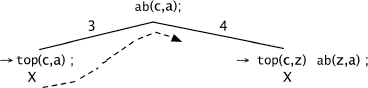
X: problem impossible to solve

The program halts and answers No.

b)

1) P(a, b) →;

2) P(c, a) →;

3) P(x, y) → P(x, z) P(z, y);

P(u, b); % the question

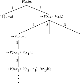
Of course this problem has two solutions u = a and u = c, …but only the first one is found. To try finding all the solutions, we can swap the orders of clauses 1 and 2, or swap literals P(x, z) and P(z, y) in clause 3. In both cases, after having found both solutions, the program does not halt.

It is suggested to use the following technique:

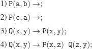
Q(u, b) % the question

DIGRESSION 12.1.– When transforming programs, it is natural to wonder whether they are equivalent, and in the case of logic programing, this boils down to ask whether one program is a logical consequence of another one.

We seize this opportunity to show the usefulness of automated theorem provers (or proof assistants) for programing. We have used one of the best-known provers based on the resolution method (Prover9), which contains a tool capable of constructing finite models (Mace4).

If we let P1 stand for the initial program and P2 stand for the suggested program, we show that P1 is not a logical consequence of P2 (by exhibiting a counter-model constructed by Mace4). However, if the implication of clause 3. of the modified program is replaced by an equivalence, which yields, say, P2', then we give a proof that P1 is a logical consequence of P2'.

EXERCISE 6.2.– The intended meaning of the terms:

a: 0

s(x): successor of x (in )

a)

add(a, x, x) →;

add(s(x), y, s(z)) → add(x, y, z);

b)

mult(a, x, a) →;

mult(s(x), y, u) → mult(x, y, z) add(z, y, u);

c)

less(a, s(x)) →;

less(s(x), s(y)) → less(x, y);

d)

divides(x, y) → not(eq(x, 0)) division(y, x, z);

division(y, x, z) → mult(z, x, y);

% not: see section 6.3.2.

e)

prime(x) → not(eq(x, 0)) not(eq(y, 1)) less(y, x) not(divides(y, x))

% eq: see exercise 6.10

% not(eq(y, 0)) not necessary because in divides

EXERCISE 6.3.– The intended meanings of the terms:

a: 0

s(x): successor of x (in )

EXERCISE 6.4.–

The regular expression that characterizes the sequence of applications of the resolution rule with the strategy used by the interpreter PL (each application is represented by the used mgu):

The application of a gives the first solution, the rest of the regular expression gives the other solutions.

EXERCISE 6.5.–

a)

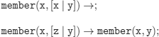
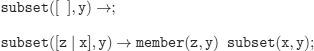
append

append

b)

c)

palindrome(x) → reverse(x, x);

d)

Other definition (program):

e)

f)

We give three definitions (programs).

i)

ii)

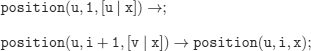
position(x, n, y): element x is at position n in list y

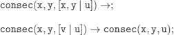
consec(u, v, x) → position(u, i, x) position(v, i + 1, x);

iii)

consec(u, v, x) → append(y, [v | z], x) append(w, [u], y);

Idea:

EXERCISE 6.6.– We first define the predicate partition

partition(list_ L, element_ of_ L (x), list_ of_ smaller_ elements_ than_ x_ in_ L, list_ of_ greater_ elements_ than_ x_ in_ L)

EXERCISE 6.7.–

% We identify adjacent elements:

% {a => b} is a constraint whose meaning is obvious. It could be replaced by a predicate similar to that of exercise 6.2 (c).

EXERCISE 6.9.-

a)

b)

EXERCISE 6.11.–

EXERCISE 8.1.– We prove properties that will permit us to simplify the answers to points (a) and (b).

We choose to represent clauses as sets of literals and recall that the sets of variables of distinct clauses are disjoint (see definition 5.10).

Property 1: let denote a substitution:

PROOF.– By definition of a subsumption, there exists a substitution such that:

The application of a substitution to a clause cannot change the number of its literals (see definition 5.12); hence, by applying an arbitrary substitution to C and to D, the set inclusion cannot change: will act in the same way on C and on the corresponding subset of literals in D (as it is the same!). We can thus write:

there therefore exists a substitution (i.e. o ) such that:

hence (definition of a subsumption):

We have the following immediate consequence.

Property 2: let C and D denote two clauses such that Var(D) = {y₁,y₂,…, y_n} and let be the substitution:

where the a_i’s (1 ≤ i ≤ n) are constants distinct from those in C and D (intuition: the constants occurring in C and D already have an intended meaning, and to reuse them could change this meaning),

if C ≤_s D, then C ≤_s D

PROOF.– Trivial, by applying property 1 with instead of .

The following property is a property that will be very useful to answer points (a) and (b).

Property 3: let be the substitution of property 2.

C ≤_s D iff C ≤_s D

PROOF.– only if property 2

if

there therefore exists a substitution such that:

Assume Var(C) = {x₁,x₂,…, x_m}

and and t_i is a closed term for 1 ≤ i ≤ m because D is a closed clause)

Of course, all the names of the literals (i.e. the predicate symbols) in C are in D (as and do not act on the predicate symbols).

To prove C ≤_s D, we must get back to D, or in other words, undo what was done by .

We thus define the operation:

meaning: “s_i is the term obtained by replacing in t_i constant c_i by variable y_i (1 ≤ i ≤ n)”.

Consider the substitution:

and let Ω = [c₁ |y₁,c₂ |y₂...,c_n | y_n] (Ω is not a substitution; hence, the different notation)

By construction: Ω(D) = D

and also by construction δC⊆D.

As a small example of these constructions, let (as usual x, y denote variables and a, b denote constants):

hence C ≤_s D.

Property 3 allows us to replace the study of C ≤_s D by the study of C ≤_s D_f, where D_f is a closed clause.

We use this property to answer the question.

a)

The clauses are disjunctions of literals with all variables quantified universally.

If C ≤_s D, then there exists a closed substitution that transforms C into a subclause of the closed clause D.

Every model of C evaluates C to T on all elements of the domain, in particular, on the elements denoted by the closed terms that replaced the variables of C (functional symbols are associated to total functions, see definition 5.6).

Hence, every model of C is a model of D and

if C ≤_s D, then C D.

b)

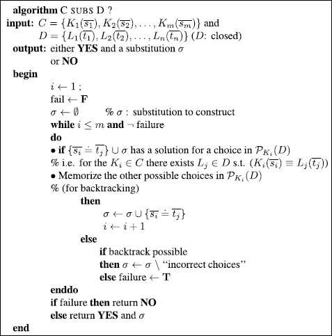
To answer question (b) it suffices to recall the definition of a subsumption and note that there exists an algorithm (UNIFICATION) that permits us to solve sets of equations on terms.

An (inefficient!) decision procedure could be that of Figure 12.1²:

We consider the input clauses, say C and D, as sets of literals:

D: closed clause, meaning that the occurrence test (rule 7 of algorithm unification is not necessary (see exercise 4.1 d)).

We note , the set of literals of D whose names (predicate symbols) are the same as the name of K_i (of course, every literal name in C is a literal name in D, otherwise, the negative answer to the subsumption test is immediate).

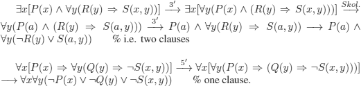
EXERCISE 9.1.– As we have to prove validity, we negate the corresponding formula

EXERCISE 9.2.–

As we have to prove validity, we negate the corresponding formula:

EXERCISE 9.4.–

% The closed world:

% The possible positions:

We also give a schema of propositional formulas that permits us to get the specification in PL of the n-queens problem for all n .

The proposition schemas P_i,j mean: a queen is at the intersection of line i and column j.

or the equivalent schema:

where the disjuncts of the schema have the following meaning:

: queen on a square of the same line;

: queen on a square of the same column;

: queen on a square of the same diagonal NE-SW going through i, j;

: queen on a square of the diagonal NW-SE going through _i,j,

EXERCISE 9.6.– R is a well-founded relation, meaning that there are no infinite sequences {a_i}_i such that R(a₁,a₀), R(a₂, a₁),…, R(a_n+1,a_n),...

This is explained by taking:

P set of elements (⊆ D)

P(x) x P

The formula is interpreted as follows.

Every non-empty subset of the domain [∀P(∃xP(x)…] contains an element [ ∃zP(z)…], such that there is no other element in the subset that is in relation with it [ … ∀y(P (y) R(y, z)…].

b)

Connected graph

This is explained by taking

C set of nodes (⊆ D)

C(x) x C

A(x, y) there is an edge from x to y

The formula is then interpreted as follows:

For every non-empty subset of nodes [ ∀C((∃xC(x)...], if x is in the subset [... C(x)...] and if when there is an edge from x to y, then y is also in this subset [... ∧ A(x, y) C(y)...] and all the nodes in the graph are in this subset [... ∀zC(z)...].

c)

Non-connected graph with connected components

This is explained by taking:

C set of nodes (⊆ D)

C(x) x C

A(u, v) there is an edge from u to v

The formula is then interpreted as follows.

There exists a non-empty subset of nodes of the graph [ ∀C((∃xC(x)...], which does not contain all the nodes in the graph [... ∃y... ¬C(y)... (disconnected part)], and such that if a node belongs to this subset [... C(u)...] and there is an edge from this node to another one [... A(u, v)...], then the latter is also in the subset [... C(v)... (connected part) ].

EXERCISE 10.1.–

a)

C = A B, by definition:

by definition:

1) A ⊆ C and B ⊆ C

Let D such that:

2) A ⊆ D and B ⊆ D

then:

i.e.:

by definition:

3) D = C

From (1), (2) and (3) we conclude that C is the smallest set containing A and B.

b)

C = A B, by definition:

by definition:

4) C ⊆ A and C ⊆ B

Let D such that:

5) D ⊆ A and D ⊆ B

then:

i.e.:

by definition:

6) D = C

From (4), (5), and (6), we conclude that C is the greatest set contained in A and B.

c)

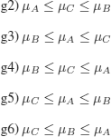
(For every x) we arrange in decreasing order

By transitivity of order relations:

where i, j, k {A, B, C}

d)

similar (with min)

e)

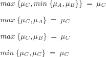
There are two possible cases

e1)

We verify easily that:

e2)

Similar.

f)

Analogous to (e), by verifying:

g)

The property to verify here is:

which must be verified for the 6 (= 3!) possible cases:

g1)

We verify for (g1)

h) Analogous to (g) by verifying:

EXERCISE 10.2.–For example:

EXERCISE 10.3.–

a)

Let R ⊆ A × B and S ⊆ B' × C

If then for every pair (x, y)

If , then we must keep the pairs containing the z’s that are in B and in B', i.e.:

and regroup all these values:

b)

c)

d)

In classical logic: if xRy and yRx, then x = y

We can propose:

or:

e)

In classical logic: if xRy and yRz, then xRz

The idea is that x will be related to z at at least the same degree as x and y are related (which corresponds to min).

EXERCISE 10.4.–Yes:

and and not C and not D and not very D and not very true and not very true and not not very true and not not very true and not very not very true and not very false

The semantics:

EXERCISE 10.5.–

a)

b)

c)

d)

e)

f)

g)

h)

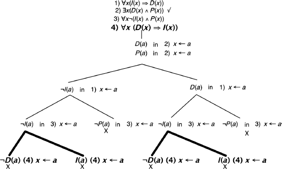
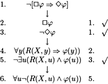
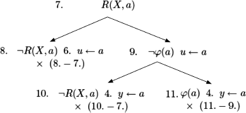
EXERCISE 10.6.– For the first of the translations in modal logic, it is possible to verify the soundness without translating the formula into FOL. Indeed, consider the set of the three premises and the negation of the conclusion (clauses (1) to (4) at the root of the tree).

We show that the other translation does not correspond to a correct reasoning, by constructing a counter example using the translation method and the method of semantic tableaux. As usual, we consider the set of premises and the negation of the conclusion.

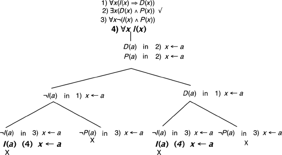
In bold , we can read a counter example of this formalization of the argument (reasoning) of the sea battle.

EXERCISE 10.7.–

a)

If R is total, i.e. , we have R(X, a) (by assigning ) and we can graft the following tree:

b)

If R is Euclidean, i.e. , then we have and we can also close the left-hand branch.

c)

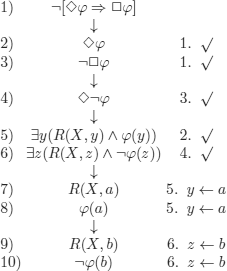
If R is functional (“unique”), i.e. ,

then we have a = b (7 - 9) and the tree can be closed (8 - 10)

d)

If R is shift-reflexive, i.e. , then we have R(a, a).

We can thus close the tree by grafting to the open branch the tree:

e)

Line 12' corresponds to R confluent (or convergent), i.e.

EXERCISE 10.8.– If we keep the semantics of in definition 10.9:

EXERCISE 10.9.–

a)

The underlined formulas at time t_i are those produced by the application of a rule at time t_j (j < i).

The tree is closed, hence the formula is valid.

b)

The formula is not valid. counter example:

which could translate into: “if it will rain and the weather will be cold, that does not mean it will rain and the weather will be cold at the same time!”.

EXERCISE 10.10.– We can find representations in the literature similar to the representation below. It is explicit enough. The reader can name the instants for each group of formulas.

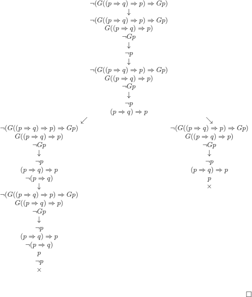
EXERCISE 10.11.– The rule corresponding to

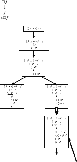
The underlined formulas are those that were developed in the parent node (rectangle).

---

1 We exclude the truth value assigned to the corresponding formula from the line.

2 This is a specification destined simply to show that a decision procedure exists, and is in no case intended to be implemented.