Chapter 3

Propositional Logic

The first logic we shall study is propositional logic (PL or PC), and although this logic has a limited expressive power, its wide variety of applications along with its role in the foundations of automation of first-order logic makes it an essential topic to study.

DEFINITION 3.1.– (proposition 1). A statement or an expression (i.e. a syntactically correct sequence of characters) that expresses a relation between several objects (terms) is a proposition.

For most of the material in this course, the following definition will be sufficient.

DEFINITION 3.2.– (proposition 2). A proposition is a statement or expression to which one (and only one) true value can be assigned.

REMARK 3.1.– Later on (see section 10.1), we shall see other possible values that can be assigned to a proposition.

EXAMPLE 3.1.– (declarative and imperative sentences).

“The factorial of 0 is 1” is a proposition.

“The factorial of 1 is 1” is a proposition.

“The factorial of n(n > 1) is n - 1 times the factorial of n - 2” is a proposition.

“Go to label LAB” is not a proposition.

“Store value 3 at the index labelled by x” is not a proposition.

We shall use two approaches to study PL (one semantical and the other syntactic). In both cases, we need a language.

3.1. Syntax and semantics

The key notion in the semantical approach is that of interpretation. In the syntactical approach (see section 3.3), it will be that of symbolic manipulation (which implies: independent of all meaning).

The language is the one defined by the syntax of PC (PL).

DEFINITION 3.3.– The only accepted formulas are the ones with a syntax compliant with the rules given below. They are called well-formed formulas, or simply wffs.

Let Π denote a denumerably infinite set of basic formulas (or atomic formulas, or elementary formulas, or propositional symbols) that shall be noted, for example, P₁, P₂, …, or P1, P2, …, or P, Q, R, ….

The set of propositional formulas (denoted by is the smallest set containing the elements in Π, which is closed for the rule:

If and are propositional formulas, then:

, and are also propositional formulas.

, ∧, ∨, , and ⇔ are called logical connectives or simply connectives.

The hierarchy (or priority) of connectives is, in decreasing order (which means that negation is the first to be applied):

negation

∧ conjunction

∨ disjunction

implication

⇔ equivalence

For one same operator: from left to right.

For example:

is the same as

REMARK 3.2.– (the set of wffs of PL is denumerably infinite). The set of wffs of PL is denumerably infinite: there are many basic symbols denumerably infinite and it is possible to come up with a procedure that enumerates wffs.

Every infinite set of wffs of PL will be a subset of a denumerably infinite set, and will therefore also be denumerably infinite.

DEFINITION 3.4.– (semantics of PL (of PC)). An n-ary truth function is a function:

Among the possible binary truth functions, the following set of connectives is usually used: {, ∧, ∨, , ⇔}. It is sufficient to express all possible binary functions (see exercise 3.2).

DEFINITION 3.5.– Let Π denote the set of basic formulas in the language. An interpretation I is a function:

Practically speaking, we shall generally be interested infinite sets of formulas, and it will suffice to consider Π restricted to the basic formulas occurring in the formulas under consideration (see definition 3.8).

EXERCISE 3.1.– How many interpretations are there for PL:

1) A finite number?

2) A denumerably infinite number?

3) An uncountably infinite number?

DEFINITION 3.6.– (interpretation of non-elementary wffs: truth tables). We define , the extension of I to the set of propositional formulas, as follows:

1) if A is an atomic formula

2)

3)

4)

5)

6)

(A), which shall also be noted as (A, I), is similar to the well-known truth tables

REMARK 3.3.– Compare these with the inference rules of semantic tableaux (see section 3.2).

REMARK 3.4.– (history of truth tables). The introduction of truth tables in modern logic is attributed to C.S. Peirce, who borrowed them from Stoicians (4th Century BC), and they have also been attributed to L. Wittgenstein.

We know that they were also known by the Megarians (school of philosophy founded by Euclid of Megara, 5th to 4th Century BC), and, in particular, we know that Philo of Megara proposed truth functions. This school, to which Eubulides belonged (see example 8.1), was interested in “everyday” argument and in paradoxes.

Truth tables were a means to decide the truth value of any wff.

The translation of sentences from everyday language to the language of PC comes with its share of problems, and we must be cautious and take into account, for example, the habits of a given language.

EXAMPLE 3.2.–

If we wished to translate the (most probable) semantics of (a), we would use ⇔ (but not ) because according to habits, what we mean is “if it rains, then I will go to the movies, and if it does not rain, then I will not go to the movies”.

(b) Should of course be translated using and exclusive or.

If A then B can be translated by (A B) ∧ (¬A ¬B).

When we say “some P are Q” we also mean “some P are not Q”.

In logic (as in mathematics), we assume that premises are interpreted in a minimal way, that is, if P then Q is translated by P Q; there exists x such that, we assume there exists such an x, etc.

Just as in the case of a function, we can define the extension and the restriction of an interpretation.

3.1.1. Language and meta-language

is valid, that is, every interpretation of is a model of (one such example is : A ∨ ¬A).

every model of is also a model of

(one such example is : A and : A ∨ α with ).

REMARK 3.5.– Note the difference between and . is a symbol of the language, whereas is a symbol of the meta-language.

The notation F means “interpretation is a model of F”.

The notation G, or equivalently (see exercise 3.14) , means “interpretation is a model of F and G”

Although it is trivial, the following meta-theorem is very important.

META-THEOREM 3.1.– iff

is unsatisfiable (or contradictory, i.e. impossible to evaluate to T).

Since the origin of logic, the interest of considering sets of truth values other than {T, F} has been widely acknowledged.

Among others, linguists propose examples of propositions such as:

The current king of France is bald.

The current king of France is not bald.

Michael (who has always been a vegan) stopped eating meat.

Michael (who has always been a vegan) did not stop eating meat.

that are neither T nor F.

Although we shall not mention logics with more than two truth values before Chapter 10, we show an example of a truth table for a logic with three truth values, the value ⊥ denoting an indeterminate value.

EXAMPLE 3.3.– (truth tables with partial information (Kleene)).

DEFINITION 3.7.– A set of connective is adequate iff it permits to express all truth functions.

EXERCISE 3.2.– Prove that the sets of connectives below are adequate. More precisely, design an algorithm that takes an arbitrary truth table as an input (graph of a truth function), and as an output produces the same function, defined using a wff constructed with (exactly) the same propositional variables and (exclusively) the given set of connectives.

EXERCISE 3.3.– A wff of PL is positive if it contains only propositional symbols and the connectives ∧ and ∨.

Consider an n-ary truth function

such that:

f (F, F, …, F) = F %, that is if all its arguments are F then its value is F;

f(T, T, … T) = T %, that is if all its arguments are T then its value is T.

f is the truth table of a positive wff of PL.

Do you believe:

EXERCISE 3.4.– Give the truth tables of the following wffs:

EXERCISE 3.5.– Answer questions (a) and (b) given below without entirely constructing the truth tables and without applying any transformation to the formula. This exercise is an introduction to a method that will be studied in section 3.2.

The following definitions (that were regrouped for the sake of simplicity) introduce some fundamental notions:

DEFINITION 3.8.– (important concepts and terminology). (The definitions of interpretations and evaluations have already been presented, but they are repeated here so that they can be regrouped with other definitions).

– A wff F is in negative normal form (nnf) iff the negation symbols that occur in F are exclusively applied to atomic formulas.

– A wff is in conjunctive normal form (cnf) or in clausal form iff it is of the form:

where each C_i is called a conjunct (or a clause)¹ and is of the form:

where A_i ≠ A_j for i ≠ j (clauses are also defined as sets of literals).

The length of a clause is the number of literals it contains.

A clause of length 1 (i.e. m_i = 1) is called a unit clause.

The cnf is associated with the set of clauses {C₁, C₂, …, C_n}.

– The wff is in disjunctive normal form (dnf) iff it is of the shape:

where each D_i, is called a disjunct and is of the form:

For homogeneity reasons, we shall allow conjunctions (disjunctions) of empty sets. In this case, the conjunction (disjunction) will not add any symbol to the syntax of the wff it occurs in.

– In both cases, A_j is a propositional atom (i.e. a basic propositional symbol) or the negation of a propositional atom, and will be called a literal.

– If L (respectively, ¬L) is a literal, then ¬L (respectively, L) is called the complementary literal of L (respectively, ¬L). It is denoted by L^c.

L is a positive literal and ¬L a negative literal.

We will also talk of the sign of a literal (respectively, positive and negative).

– If all literals in a clause are positive (respectively, negative), then the clause is positive (respectively, negative).

– A wff G is the cnf (respectively, dnf) of a wff F iff G and F are equivalent (i.e. F ⇔ G is a tautology, see below), and G is in cnf (respectively, dnf).

– An interpretation I of a language (a wff ) is an application:

where Π is the set of propositional symbols (basic formulas, atomic formulas, and elementary formulas) of the language (of ). If the domain of the interpretation is restricted to a proper subset of Π, then I is a partial interpretation

In particular,

– The interpretation of a formula (respectively, of a set of formulas ) is the restriction of the language that (respectively, ) belongs to the set of propositional symbols of (respectively, ). This set will generally be denoted by Propset() (respectively, Propset()).

– A partial interpretation of a formula is the restriction of the interpretation of the language that belongs to a set in which Prospect().

– An evaluation of a wff for an interpretation I is the truth value of for I. It is denoted by ( I) and sometimes by ().

– A model of a wff (a set of wffs ) is an interpretation I of (of ) such that . We say that I satisfies ().

– A counter model (counter example) of a wff is an interpretation I of (of ) such that for at least one ∈ ). We say that I falsifies ().

– A wff is satisfiable or consistent or coherent iff it admits (at least) one model.

– A wff is unsatisfiable or contradictory iff it admits no models, that is, for all I: .

– A wff is valid or tautological iff for all I: .

We note .

– A wff is a logical consequence of a wff denoted by , iff every model of is a model of .

These definitions naturally extend to sets of wffs.

We can therefore write or, as is more common, .

EXERCISE 3.6.– For F, G in , we define the binary relation iff .

Is an order relation? (Also see definition 3.26)

How can interpretations be specified? The following example shows three common ways to do so.

EXAMPLE 3.4.– Consider the following formula:

(1), (2), and (3) given below are three different notations that specify the same interpretation²,

1)

2)

3) I = {C, E} (here, only those propositions that evaluate to T are mentioned)

For notations (1) and (2):

1) If < P, T > (respectively, < P, F >) ∈ I then < P, F > (respectively, < P, T >) ∉ I

2) If P (respectively, ¬P) ∈ I then ¬P (respectively, P) ∉ I

(I is an application). Of course, this remark is not necessary for notation 3.

EXERCISE 3.7.– Verify that the following formulas (paradoxes of material implication) are tautologies:

Do they have a translation in everyday language?

REMARK 3.6.– The following tautologies are often used in mathematics, in the statement of theorems:

EXERCISE 3.8.–

– Is the following reasoning (or argument) correct?

– How can a correct reasoning be characterized? In other words, what relationship must hold between the premises and the conclusion for the reasoning to be correct?

– Using your definition of a correct reasoning, can you verify that the syllogisms of example 2.12 are correct reasonings?

If life has a meaning, but necessarily ends by death, then life is sad.

If life goes on after death, but does not have a meaning, then life is a cosmic joke.

If life had a meaning and went on after death, then angst would not exist.

If life is not a cosmic joke, then it is not sad.

Angst exists.

If life is sad or if it is a cosmic joke, then it is not beautiful.

Therefore life is ugly.

REMARK 3.7.– Perhaps here is the best place to recall the following quote from Wittgenstein: “Logic is a vast tautology that does not state anything about the world, it simply expresses the equivalence between propositions”.

A reasoning is a set of premises and a conclusion. Reasonings are usually represented by a column of premises that are separated from the conclusion by a horizontal line.

EXERCISE 3.9.– Are the following reasonings correct?

The notion of the normal form of a formula is very important for at least two reasons: the first one is that it permits us an economy of thought, as we can always assume (once we have proved the existence of this normal form) that the formula under consideration is already under normal form. The second reason is that when this normal form is unique, we can prove the equivalence (equality) of syntactically different formulas by a reduction to this normal form.

In definition 3.8, we introduced two normal forms for formulas in propositional logic: the cnf and the dnf. The following rules allow us to obtain these normal forms.

3.1.2. Transformation rules for cnf and dnf

– Step 1: elimination of ⇔ and ⇔

1)

2)

– Step 2: put ¬ next to the atoms

1)

2)

3)

– Step 3: distributivity of ∨ and ∧

1)

2)

The following rules are often used:

REMARK 3.8.– (3-cnf). We can prove (by adding propositional variables that are used to introduce definitions) that every cnf formula F can be transformed into another cnf F_≤3 with at most three literals in every clause, such that F_≤3 is satisfiable if and only if F is satisfiable.

EXERCISE 3.10.–

REMARK 3.9.– Sometimes the transformation rules generate redundancies that can potentially (and artificially) increase the search space of a method using a normal form, as shown in the following example:

The conjuncts that are underlined are tautologies that could be eliminated from the start by introducing a new rule:

Note that in the analysis of deductive argument performed below, two different strategies (or any combination of the strategies) can be considered. The word strategy means ordering and decrease (if possible) of the number of choices in non-deterministic problems (see section 3.8.1):

– forward chaining (bottom up): starting from the premises and by application of the inference rules (or by using the meaning of connectives), try to reach the conclusion. We have not yet defined what inference rules are (see definition 3.9), but for the time being it is sufficient to consider them as elementary reasoning steps (which corresponds to the formal definition). The important thing is to declare the elementary reasoning steps that is allowed to use.

We move from the premises to the conclusion.

– backward chaining (top down): starting from the conclusion (denoted by C) reason by saying: if we want to have C, it suffices to have A, if we want to have A, it suffices to have B, etc., and if possible, move to the premises.

We move from the conclusion to the premises.

EXERCISE 3.11.– Is the following reasoning correct?

If there is a unique norm to judge greatness in art, then both M and G cannot be great artists. If P or D are considered as great artists, then W is certainly not one. However, if W is not a great artist, then K or S are not great artists either. After all, G is not a great artist, but D and K are.

Therefore, there is no unique norm to judge greatness in art.

EXERCISE 3.12.– Imagine a reasoning that is presented as usual by a set of premises and a conclusion. The premises and the conclusion are wffs of propositional logic.

Propset(set – wf f) is the set of propositional symbols in the set of wffs set – wf f.

a) Assume that Propset (premises) ∩ Propset (conclusion) = ∅. Can the reasoning be correct?

If this is not the case in general, are there particular cases in which this property holds?

b) Now imagine that the premises and the conclusion are in clausal form (see definition 3.8). This assumption does not incur any loss of generality (why?).

Given a set of clauses, a literal (see definition 3.8) whose negation does not occur in the other clauses is called a pure literal.

If a premise contains a pure literal, can the analysis of the reasoning be simplified? How?

EXERCISE 3.13.– A crime occurred in a luxurious home and the police inspector in charge of the investigation reasons as follows:

If on the day of the crime, someone had asked the house servant the question “Why were you not at dinner the day before yesterday?”, she would have answered.

If she had answered, someone would have heard her.

The house servant was not heard.

If the house servant was neither seen nor heard, that is because she was polishing cutlery, and if she was polishing cutlery, then she was here on the day of the crime.

I, therefore, conclude that the house servant was in the house when the crime occurred.

a) What premise(s) should the police inspector have added for the reasoning to be correct?

b) Is there a unique possibility?

c) Can a correct reasoning be made incorrect by adding premises?

The proof of the following meta-theorem is trivial.

META-THEOREM 3.2.– A is valid iff ¬A is unsatisfiable (contradictory).

EXERCISE 3.14.– Prove the following meta-theorem (deduction theorem-semantical version):

We will be interested in expressions of the form:

where the H_i’s (1 ≤ i ≤ n) and C are wffs.

These kinds of expressions correspond to the informal notion of a correct reasoning.

EXERCISE 3.15.– Prove the following meta-theorems:

a)

Note that in mathematics, we usually write:

with the implicit meaning:

.

b) is unsatisfiable.

We will sometimes use the set-theoretical version of this statement: C is a logical consequence of {H₁, H₂,..., H_n} iff {H₁, H₂,..., H_n, ¬C} is unsatisfiable.

(This last meta-theorem is the well-known reductio ad absurdum proof technique: reaching a contradiction by negating the conclusion.)

We have seen (see exercise 3.12) that what is of interest in a non-trivial reasoning are the propositional symbols that occur on the left-hand side and the right-hand side of : their interpretation on the left-hand side (respectively, right-hand side) fixes their interpretation on the right-hand side (respectively, left-hand side).

EXERCISE 3.16.– By assuming that:

%, that is, not all models of are models of ,

and

.

Which of the following assertions is correct?

EXERCISE 3.17.– Let S denote a finite set of wffs S = {f₁, f₂,... f_n}.

Assume that S is minimally unsatisfiable (i.e. S is unsatisfiable, and every proper subset of S is satisfiable, see also definition 3.18).

Is the following assertion true or false?

We can identify n correct reasonings with premises and conclusions that are formulas in S or negations of formulas in S.

META-THEOREM 3.3.– (interpolation theorem). , , and denote wffs of propositional logic.

Propset (): set of propositional symbols in wff .

if:

then:

EXAMPLE 3.5.– Q ∧ R P ∨ Q

Q ∧ R Q and Q P ∨ Q

here : Q ∧ R : P ∨ Q : Q

EXERCISE 3.18.–

Compute the interpolant(s) of:

3.2. The method of semantic tableaux

We have characterized a correct reasoning (from a semantical point of view) as a reasoning in which there is no interpretation that evaluates the premises to true and the conclusion to false (simultaneously). As a consequence, if we try to construct all possible models of the set of premises and of the negation of the conclusion, then we are “killing two birds with one stone”. Indeed, if we do not succeed, then we were unable to refute the reasoning, because we were unable to evaluate the premises to true and the conclusion to false (as we tried to evaluate the negation of the conclusion to true). Hence, the reasoning is correct. However, if we succeed, then we will have produced a counter example that proves the reasoning is not correct.

We also noticed that it is not always necessary to construct an entire truth table to evaluate a formula to true (see exercise 3.5).

These ideas form the basis of a method that is used not only in a propositional logic but that also extends to first-order logic, to modal logics, etc.

The method of semantic tableaux, of which many variants are available, is a formalization of these ideas. It is based on the following technique: for every connective (formula constructor) that can occur in a wff , we provide all the ways of constructing models of . Of course, these possibilities are encoded in the simplest possible way.

The set of connectives that are used is {¬, ∧, ∨, , ⇔}, and the method uses the following rules ( and denote wffs):

Type α rules (wffs with only one descendant)

Type ß rules (wffs with two descendants)

Intuition behind the method: given a set S of wffs and using the rules above, we try to construct all the models of S by combining the models of each formula.

It is clear that the rules replace wffs by wffs containing (strictly) less symbols; thus, we necessarily reach literals (this property is used to prove the termination of the method).

The combination of models translates into a tree (which is not unique and depends on the order in which the models of S are analyzed).

Some combinations may not be possible (because we are trying to evaluate an atomic formula to true to construct the model of one wff, while evaluating it to false to construct the model of another one). As soon as a branch contains literals A and ¬A, it is closed (to close a branch, we will use the symbol ×). We shall say that the branch is closed. If a branch is not closed, then it is open.

A tableau is closed iff all its branches are closed. It is open otherwise.

Before providing the corresponding algorithm, we apply the rules on a few simple examples.

In agreement with what we said at the start of the section, we consider the set (which means that there is no imposed ordering to analyze the formulas) of formulas:

We will try to construct a (several) model(s) for the set of formulas (1), (2), and (3). The order selected for the analysis is (3), (1), and (2). The procedure is:

Conclusion: All the branches in the tree are closed. This means that we have failed to construct any model of (1), (2), and (3). This set of wffs is therefore contradictory (or unsatisfiable, or incoherent). The original reasoning was correct (see exercise 3.15).

Consider the following reasoning:

We analyze the set:

We choose to apply the rules in the order (2), (1).

We have analyzed two examples of correct reasonings. What happens when a reasoning is not correct? Is the method also useful? Consider the following reasoning:

We therefore consider the following set of wffs:

and we choose to analyze it in the order (3), (2), and (1).

As we are trying to enumerate all the potential models of the set of wffs under consideration, in principle, we should have grafted the subtree with root ¬Q instead of ×, but of course, this is not necessary because all the branches starting at this node will contain the contradiction (R, ¬R).

What do open branches mean? By reading the atomic wffs and the negations of atomic wffs, we obtain the models of the premises and of the negation of the conclusion; hence the models of the premises are counter models of the conclusion, i.e. counter examples showing that the reasoning is not correct.

The counter examples that we can read on the open branches are:

REMARK 3.10.– It should be clear that the method of semantic tableaux for PL (PC) is a method for enumerating the models of a set of formulas, and thus permits us to decide the (un)satisfiability ((in)coherence) of a set of wffs.

EXERCISE 3.19.– Use the method of semantic tableaux to prove that the set of formulas below is unsatisfiable (contradictory or incoherent). Use two different analysis orderings to show that the size of the tree depends on the ordering.

3.2.1. A slightly different formalism: signed tableaux

This formalism will be useful for logics other than classical logic, which we are currently studying. It speaks sufficiently for itself to require any explanation.

We want to prove the validity of the following wff (i.e. prove that it is a tautology: it is evaluated to true in every interpretation):

we therefore consider the wff:

which leads to the following tableaux:

REMARK 3.11.– This formalism may seem redundant in bi-valued logic, its utility will become obvious in multi-valued logics (see section 10.1).

Normally, several questions arise at this point of the presentation of the method of semantic tableaux, to which answers must be provided in a systematic study of the topic. The order of the questions is not related to their importance.

1) Must the conclusion (or the formula if there is only one) be negated to test its validity?

2) Are the constructed trees always finite?

3) What is the termination criterion?

4) When the method states that a reasoning is correct, is this really the case? (If so, the method is correct).

5) Can all correct reasonings be detected with this method? (If so, the method is complete).

6) Is the order in which the formulas (or sub-formulas) are analyzed important?

We begin by answering YES to question 1.

The method of semantic tableaux was created to enumerate all models of a set of formulas (and in particular, of sets containing only one formula).

By definition, if S is a set of wffs:

– set of models of S ⊆ set of interpretations of S;

– set of (all the) valid wffs ⊂ set of (all the) non-contradictory wffs.

If no negation is performed, then all models are enumerated, but we do not know anything (without some additional reasoning) about the potential counter examples. Consider the following wff.

EXAMPLE 3.6.–

We have proved that is not contradictory, but we do not know whether it is valid.

If we negate, we try to construct all models of ¬, i.e. all counter models (counter examples) of .

EXAMPLE 3.7.–

We have constructed two models of ¬ (CE1 and CE2). CE1 ({¬A, ¬C, B}) and CE2 ({¬B, ¬C, A}) Are counter models (counter examples) of , which is therefore not valid, as we might have believed after a hasty interpretation of the tableaux in which was not negated.

REMARK 3.12.– We have indirectly answered questions 1, 2, 3, and 6 given earlier. The proposed algorithm is non-deterministic (instruction choose) and can therefore be implemented with different strategies.

EXERCISE 3.20.– Use the method of semantic tableaux to verify the (in)correctness of reasonings (a) to (f), and the (in)validity of formula (g) below.

EXERCISE 3.21.– Are the sets of wffs ₁ and ₂ below satisfiable? Unsatisfiable?

Use the method of semantic tableaux to find the answer.

DIGRESSION 3.1.– (some refreshers on trees).

– A directed graph is a structure (see definition 5.4) , where is an irreflexive relation³.

G: set of nodes; R^G: set of edges.

– A tree is a directed graph with a (unique) distinguished node r, called its root, such that:

i) no edge reaches r (i.e. );

ii) for all nodes n in the tree, there exists a unique path (branch) from r to n.

– If there is a path from a node x to a node y, then y is a descendant of x and x is an ancestor of y.

– The degree of a node is the number of outgoing edges of the node.

– A node of degree 0 is called a terminal node, or a leaf.

– The length of a branch is the size of the set of its nodes.

– A tree is infinite iff it has infinitely many nodes.

– A tree is finitely generated iff all its nodes have a finite degree.

REMARK 3.13.– (other definitions of a tree). A tree is a partially ordered set (with order relation , see definition 3.24) satisfying the additional axiom:

(this means that the set of minorants of each element is totally ordered).

THEOREM 3.1.– (König’s lemma). If A is an infinite tree that is finitely generated, then A contains (at least) an infinite branch.

or

If A is a tree with only finite branches then A contains a branch of maximal length.

or If for all there exists a node of depth n, then A contains an infinite branch.

König’s lemma does not apply to trees that are not finitely generated, as shown in the example below:

3.3. Formal systems

The notion of a formal system is closely related to the notion of proof.

3.3.1. A capital notion: the notion of proof

The notion of a proof is extremely important and subtle. It is thus very hard (and perhaps impossible) to grasp its meaning by simply relying on a formal definition. It occurs in many domains, in exact science (mathematics, physics, biology, chemistry, etc.), in social science (history, paleontology, sociology, etc.), and in many order activities that are proper to organized societies (justice, police, sales, insurance, etc.).

Etymologically:

proof → to prove → from probus: of a good quality, honest, loyal

The requirements to identify an object as a proof and the methods to carry out proofs are of course generally very different and depend on the period under consideration (including for mathematics).

For example, it is currently acknowledged in the so-called civilized societies that every individual is innocent until proven guilty.

This was not the case in the code of Hammurabi (King of Babylon, ∼1750 BC). The defendant would be thrown into the “holy river”: if he could escape unhurt, that was a proof that he was innocent; if he sank, that was a proof that he was guilty. This proof method, along with other torture methods, were used by the Inquisition during the Middle Ages.

Myths used to be considered as true, and anyone who would doubt them had to prove the contrary.

In mathematics, the acceptance of what a proof is can also be analyzed from a historical point of view. For example, pre-Euclidean proofs were much less rigorous than post-Euclidean ones. A similar remark holds for mathematical analysis before and after Weierstrass. It seems like all societies, including those considered as primitive, invented argument criteria, often as questions/answers, in particular in the domains of law and justice. Notions such as coherence are often used (but not necessarily in a conscious way) in the evaluation of arguments. An argument that tends to establish a fact (or situation) that has not been observed or to reduce the uncertainties about this situation can already be considered as proof. Once again, those who pushed the study of argument the farthest were the Greeks, in particular, between the 6th and 4th Century BC, with major works such as Aristotle’s Organon and Rhetoric, and Euclid’s Elements. The accomplishment that we are particularly interested in is the development of axiomatizations and proofs.

There were abstract arguments, before Aristotle, with, for example, Thales, Anaximander, Xenophanes, Heraclitus, and Parmenides. People already used reductio ad absurdum, analogies, dilemmas (if p q and r s and p ∨ r, then q ∨ s is a dilemma. If p q and r s and ¬q ∨ ¬s, then ¬p ∨ ¬r is another one).

There seems to be a consensus on the fact that Parmenides was the first to propose proofs with deductive reasoning, with an irrefutable initial statement and a rigorous chain of deductions. He also proposed to divide proofs into parts, using the conclusions of previous parts as premises of the current ones (today these would be called lemma-structured proofs).

The influence of these thinkers on the development of philosophy and science was huge. To better understand the social context in which the notion of a proof evolved toward its current definition, it is worth mentioning that argument blossoms much better and has a greater importance in a society in which the opinion of the citizens (who are perfectly equal) is taken into account (as was the case in Greece at the time⁴) than in an autocratic society.

Argument always takes place between two people (this is not always the case for reasoning).

Sophists, and in particular Gorgias, used the reasonings that were introduced by Parmenides and his students, not to find the truth but with a purely rhetorical goal. They believed persuasion was much more important than a proof, although the latter aims at truth and knowledge. Still, it is now acknowledged that rhetoric indirectly contributed to the progress in the concept of a proof.

Sophists also played an important role in the organization of education and in the development of a critical mind, by admitting several points of view on a same topic⁵. Socrates, who used to search for general definitions through dialog, could profit from the habits of Athenians for his teachings.

Socrates defined the art of rhetoric as the art of having influence on souls. Aristotle considered rhetoric as the technique of plausibility, but not of truth (of which proofs are the technique).

Plato must not be forgotten among those who contributed to the elaboration of the concept of proof.

Another discipline that is close to rhetoric is dialectic⁶ (instrument of probable knowledge according to Aristotle), which, according to Aristotle, is due to Zeno of Elea, was also important at the time.

It is interesting to notice that the clear separation between proving and persuading (convincing) disappears a little in philosophy and modern mathematics (see below).

Mathematics are of course the principle domain in which proofs are carried out. In a reference book (by Rasiowa and Sokorski), it is written:

The process of deducing some sentences from others is the most important part of the mathematical work.

The more common belief is that:

The first proof in the history of mathematics was produced by Thales of Miletus (600 BC): “A diameter separates a circle into two equal parts”.

As suggested by the brief historical recollection below, this notion evolved with time and it is legitimate to assume that Thales used simple and intuitive techniques.

The priority given to Thales does not seem well deserved. Indeed, one of the greatest historians of mathematics (E.T. Bell) wrote the following about Babylonian mathematics:

…More important than the technical algebra of these ancient Babylonians is their recognition – as shown by their work – of the necessity of proof in mathematics.

Until recently, it has been supposed that the Greeks were the first to recognise that proof is demanded for mathematical propositions. This was one of the most important steps ever taken by human beings. Unfortunately, it was taken so long ago that it led to nowhere in particular so far as our own civilisation is concerned, unless the Greeks followed consciously, which they may well have done. They were not particularly generous to their predecessors.

The first rigorous mathematical proofs were produced during the 5th Century BC. The concept of a rigorous mathematical proof is certainly the main difference between Greek mathematics and Babylonian mathematics.

It is worth mentioning that the ancient Greeks made a distinction between finding a theorem and finding its proof. We know that many of Euclid’s propositions were already known and accepted before his time.

The main development, of which Euclid's monumental work is the paradigm, is that of an axiomatization.

After Euclid, mathematical reasonings used definitions, common notions, and postulates.

– Common notions are the obvious principles that apply everywhere in mathematics. They are now called logical axioms. Common notions seem to contain the laws of logic (with the current meaning of inference rules).

– Postulates are the basic hypotheses on geometry (or another theory). They are now called proper axioms or non-logical axioms.

Some authors have suggested that instead of axiomatization, we should use postulation.

DIGRESSION 3.2.– The way Euclid proceeded in his work has become a standard in mathematics and other domains, among which is medicine, which was one of the first domains to incorporate it.

Galen (physician, surgeon, and philosopher of the 2nd Century) believed that mastering proofs was a prerequisite to study medicine, and he thought that everything that is proved by medical science should be reduced to prime propositions that are unprovable but held as true by everyone. This boils down to importing Euclid’s axiomatization method to medicine.

Recent research by science historians has highlighted an approach to proofs that is particularly interesting to computer scientists. Chinese mathematicians (1st Century BC) had proposed (sometimes sophisticated) algorithms to solve problems. These algorithms would provide solutions to many particular cases of the problems under consideration. Those commenting them tried to prove the veracity of the propositions, which boiled down to proving the correction of the algorithms.

At the origins of modern science (16th to 17th Century), knowledge was associated to sensitive experiments (that, just as for theories, had to be transmissible and reproducible⁷).

This is different from revelation, illumination, initiation, and hermetism as a means of discovering and transmitting knowledge.

In one of his books, Galileo mentions the imperfections of matter and the very pure mathematical proofs.

Kepler was convinced that mathematical proofs were the way to reach the truth.

Newton (following Euclid) uses the axiomatic method: he starts from the definition of mass, force, and movement. Then, he adds the presuppositions, laws, axioms. He obtains theorems, proofs, and corollaries. To get from abstract entities to a description of the world, Newton states philosophical rules.

Some mathematicians have put an emphasis on the fact that from a practical point of view, the acceptance of the proof of a theorem is a social process. There are interactions between those who propose a proof and those who verify it, detect possible errors, simplify it, make it readable, etc. The process stops when the community of mathematicians accepts (or refutes) the (alleged) proof.

Much later, the appearance of computers led to hopes and new problems about the notion of a proof. Indeed, what is more tempting than trying to prove theorems using a computer? All we have to do is to program a notion that seems completely formalized, and this led to what is considered as the first AI program: Logic Theorist (see section 7.5).

The first theorem prover that produced a mathematical proof was written by M. Davis in 1954. It was a decision procedure for Presburger arithmetic (see example 5.6). It is significant that the first problem to be tackled was a decidable one (of a high complexity): computers were used as large calculators.

However, it is only with the proof of the four-color theorem that mathematicians and the general public started talking about automated deduction.

The four-color theorem was proved using a computer program in 1976. This result is interesting for several reasons: it had been an open problem for over a century in mathematics, it had allegedly been proved by some excellent mathematicians who had produced (false) proofs (in the traditional way, i.e. without a computer), and it permitted some interesting thoughts on the notion of a proof in mathematics. This result, as well as others that followed, essentially uses the computing speed of a computer to test a huge amount of possible cases. Although the result is very important, the proof only made a very partial use of the capacities of automated theorem provers, as they are designed nowadays (in particular, no use was made of the possibilities of manipulating proofs, planning, interacting with the user to guide parts of the proofs, logical computations, etc., that are offered by modern theorem provers). It is interesting to note here the important consequences that these results had on mathematical philosophers, as an inspiration for their thoughts on mathematical practices.

The proofs that are obtained by a computer make an argument that the acceptance of a proof is a social process. The main reasons are the large number of computations that are performed (without any creativity), the lack of a perspective in the proofs (that do not distinguish those steps that are conceptually important from the other ones), and also the natural mistrust of humans toward a proof that was produced by a non-human. Let us not forget that in most cases, we “trust” competent mathematicians when they say that some assertions have been proved. It suffices, for example, to recall Fermat's last theorem.

In a reference article (by T. Tymoczko) about the implications of this work on the philosophy of mathematics, the author proposes the following thesis (that seems daring at first):

I will argue that computer-assisted proofs introduce experimental methods into pure mathematics.

To the question “What is a proof?”, the author answers by identifying three main characteristics:

– Proofs are convincing⁸

– Proofs are surveyable^{9, 10}.

– Proofs can be formalized¹¹.

Surveyability is an important subjective feature of mathematical proofs which relates the proofs to the mathematicians, the subjects of mathematical investigations. It is in the context of surveyability that the idea of “lemma” fits. Mathematicians organize a proof into lemmas to make it more perspicuous.

Other authors have almost pushed this analysis to its limit: they maintain that mathematical studies have an important empirical component (and therefore inherit its methods: reproducibility of the experiments, etc.¹²).

It is interesting to compare the theses given above with the thoughts that inspired a mathematician (C.W.H. Lam) in his own work, as he obtained new results (in 1977) using a computer. He begins his article by explaining his work, using the title of an article that had appeared in a general magazine:

Is a math proof a proof if no one can check it?

The proof involved the projective plans of order 10 and required 3000 CPU hours to a CRAY-1A, for which scientists used to believe that there were undetected (material) errors every 1000 hours approximately…!

He tries to use the expression computed result instead of “proof” and states that in the case of the proofs obtained by a computer, the assertion of correctness is not absolute, but only almost certain, which is a characteristic of a computer-based result.¹³

This kind of problem is in a close relationship to others that are clearly related to practical computer science.

For example, when we carry out a proof or a verification (e.g. for a critical system), we prove that a program is correct, which means that it will do what is expected from it on a model of a computer, but have we proved that it will do it on a real computer (that has a physical reality, with electronic components, etc.)?

On this topic, the great logician P. Martin-Löf (who influenced computer science a lot) wrote:

Now, there can be no proof, no conclusive proof, that a proof really proves its conclusion, because, if such a miraculous means were available to us, we would of course always use it and be guaranteed against mistakes. It would be a wonderful situation, but we are human beings and we are not in that position

[…]

So, clearly, there can be no proof in the proper sense of the word that a proof really proves its conclusion: the most there can be is a discussion as to whether a proof is correct or not, and such discussion arises precisely when we make mistakes, or when we have insufficient grounds or evidence for what we are doing.

The importance of the presentation (readability) of a proof (“proofs are surveyable”) cannot be overestimated:

Every result that is obtained by a means that is not surveyable by a human is not a proof.

This sentence was written by a great French mathematician (J.-P. Serre, recipient of the Fields and Abel medals).

Actually, a response to this requirement, which is not in contradiction with the acceptance of proofs obtained using a computer, is to make the following distinction along with the logician quoted above: there are proofs and there are derivations. A proof contains the computational information that a computer would need to verify a proposition. A derivation is what convinces us that a proposition is true. Derivations are what we find in mathematics textbooks. These considerations are closely related to what the same logician wrote in a brilliant article:

…Thus proof and evidence are the same. And what is it that makes a judgement evident to you? Before you have understood or grasped the judgement, it is not evident to you, and, when you have grasped it, it is obvious or evident to you. This is simply your act of understanding or grasping it which confers evidence on the judgement, that is, which makes it evident to you…

What is of a particular interest to us here is the word grasped. We cannot grasp (with our mind) extremely long sequences of symbols without any structure.

As a great logician (Y. Manin) nicely put it: “A good proof is a proof that makes us wiser”.

To conclude, recall that natural science relies (and depends on) many instruments (it suffices to consider astronomy or biology). The history of instruments, in which computers play an important part, is part of the history of science.

It is a commonplace to say that computers are indispensable for complicated numerical computations. They will probably be as indispensable as reasoning auxiliaries, to obtain (some) proofs.

3.3.2. What do we learn from the way we do mathematics?

After this brief historical perspective, we can try to rely on our direct experience of mathematics (although it is very modest) to better comprehend the topic and ask ourselves, for example:

Can we abstract common characteristics of the proofs we have discovered, read, studied, etc.?

Proofs are presented as a finite sequence of formulas, sometimes with figures (that correspond to particular cases: examples (models), counter examples (counter models)), and with sentences in natural language (generally a very restricted subset of the everyday language) that justify the introduction of new formulas, and…that’s it!

– What formulas do we begin with?: by the “unquestionable” formulas, which are admitted.

– How do we get from some formulas to others?: by some rules, generally not many of them (in general we do not bother to specify that they are the only ones we allow ourselves to use), that are implicitly correct and assumed to be natural.

We have just given the basic ideas of what we shall define as a formal system.

– The unquestionable formulas are the axioms.

– The transition rules are the inference rules.

To avoid any artificial problem (such as ambiguity), we fix a formal language.

The characterization of inference rules is more delicate than the characterization of axioms. Here are some of the most fundamental characterizations:

1) The hypothetical syllogism (modus ponendo ponens) or simply modus ponens: from A and if A then B deduce B;

2) Induction: the great mathematician Henri Poincaré (1854-1912) who was also a philosopher of science, considers induction as the fundamental mathematical reasoning tool and states that its essential character is that it contains infinitely many hypothetical syllogisms:

The theorem is true for 1

(*) But if it is true for 1 then it is also true for 2.

Therefore, it is true for 2.

(*) But if it is true for 2 then it is also true for 3.

Therefore, it is true for 3.

...

Furthermore, there is a unique formula that expresses all the formulas (*):

(*) If the theorem is true for n - 1, then it is also true for n.

The principle of mathematical induction seems to have been used in its current form by B. Pascal in 1654 in the Traité du triangle arithmétique.

From the history of science point of view, it is interesting to note that al-Karaji ((Persian) mathematician and engineer, 953 to ∼1029) used a rudimentary form of mathematical induction, by proving an argument for n = 1, then using this result to prove the result for n = 2, …, and noticing that we could go on indefinitely. He discovered what is known as “Pascal’s triangle”, using this method.

It seems like Pascal was not aware of al-Karaji’s work.

3) sometimes, we use modus tollendo tollens (or simply modus tollens):

from if A then B and ¬B deduce ¬A, which can be considered as a particular case of reductio ad absurdum (see below).

Three widely used techniques to carry out proofs are as follows:

t1) Reductio ad absurdum.

This is one of the oldest techniques. There are two cases to consider.

a) When it is used to prove that an object exists, it is closely related to the law of excluded middle. To prove P, we prove that ¬P leads to a contradiction. By the law of excluded middle, P ∨¬P is always true; hence, we may conclude that P holds. Intuitionists do not always accept these proofs because the law of excluded middle is used;

b) When it is used to prove that a mathematical object does not exist, it is accepted by all schools of thought. If P leads to a contradiction, then the object having property P cannot exist (without any other consideration).

t2) Case analysis, particularly important for proofs performed by computers, such as the proof of the four-color theorem and the projective plane of order 10.

t3) Diagonalization. This procedure was invented by Cantor and is used to perform proofs by reductio ad absurdum; we assume that we can enumerate all the objects of a class and the diagonalization procedure constructs an element of the class that is not among the enumerated objects. Assuming that there exists such an enumeration therefore leads to a contradiction (see exercise 3.1).

REMARK 3.14.– It might be useful to recall that three different theories must be distinguished:

– the informal theory, that the formal system is meant to formalize;

– the formal system or object theory;

– the meta-theory, in which the formal system is studied. The meta-theory generally corresponds to common and informal mathematics (see, for example, meta-theorem 3.4).

REMARK 3.15.– (mathematical theories). Mathematical theories can be considered from the semantic or the syntactic point of view. In the former case, the axioms have an intended interpretation (or wanted interpretation), and this model is in principle unique (see remark 5.19); for example, arithmetic, Euclidean geometry, set theory.

When the syntactic point of view is chosen, we search for those interpretations that satisfy some formulas. In this case, the number of models may be important. Examples: group theory, non-Euclidean geometry.

With the first point of view, the search for an axiomatization is similar to modeling in natural science (see Chapter 5.2).

Of course, both point of views can coexist.

In experimental science, researchers have also defined what can be considered as a proof of a scientific theory, which must include (globally) the observation of some facts, the proposal of hypotheses, and a verification (or falsification). See also sections 8.3 and 8.4.

The problems that arise with the notion of a proof in experimental science are extremely difficult (in particular, from an epistemological point of view).

DEFINITION 3.9.– (formal system). A formal system or formal theory or axiomatico-deductive system is a triplet:

where:

– is a set of wff.

is a formal language on a given vocabulary (assumed to be finite), and it can always be decided in a mechanical way whether a sequence of symbols is a word in the language (i.e. a wff) or not.

– is a finite set of inference rules, i.e. relations in .

They are generally denoted as follows:

The are called the premises, _n the conclusion or direct consequence of .

It is possible to mechanically decide whether a wff is a direct consequence of other wffs.

We may accept inference rules without premises, i.e. relations in ⁿ (n ≥ 1). In this case, the axioms are also inference rules.

The axioms and inference rules are also called transformation rules.

– ⊂ are the axioms;

– the pair = < , > is a deductive system or proof system or calculus;

– the pair =< , > is an axiomatic system or axiomatic structure or axiomatization.

The latter is the most frequently used in mathematics, and is usually not formally specified (a human is supposed to be able to recognize the wffs). There is no restriction on the inference rules that we are allowed to use. These are called informal axiomatic theories and they enable us to obtain informal proofs. In fact, it is possible to prove theorems in group theory or set theory, etc. without having ever studied first-order logic. These proofs can be considered as correct but informal (considering that these kinds of proofs are particularly important in constructive mathematics, see, for example, remark 5.29).

Nevertheless, the importance of formal (and unquestionable) proofs cannot be overstated, as they can be verified by a computer program: a proof assistant (logical frameworks).

REMARK 3.16.– A formal system is only concerned with syntax. With this syntax several meanings or interpretations can be associated. This is evidence of the importance of form in logic.

REMARK 3.17.– The principle of non-contradiction and the law of excluded middle (see section 2.2) are not inference rules. They are not properties that hold good for all considered wff.

EXAMPLE 3.8.– (arithmetic, Peano’s axioms). The set of natural numbers () has the following properties:

1) 0 ∈

2) if n ∈ then s(n) ∈ , % for all n

3) 0 ≠ s(n),, % for all n

4) if s(n) = s(m) then n = m, % for all n, m

induction axiom (see example 9.28):

5) let P denote a property on numbers.

if P(0) and (if P(n) then P(s(n))) then P(x) for x ∈ , % for all P

Sometimes the induction axiom is stated as follows:

5') if S ⊆ and 0 ∈ S and (if n ∈ S then s(n) ∈ S), then S = , % for all S

(see example 9.28).

REMARK 3.18.– (on the two statements of the induction axiom). Version 5 is weaker than version 5': as a property can be specified as a finite sequence of words in a language (defined by a grammar), only a denumerably infinite number of properties and natural numbers can be specified, but the set of all subsets of is uncountably infinite (see, e.g. exercise 3.1).

There, therefore, exist theorems on natural numbers that cannot be proved using form 5 of the induction axiom.

EXERCISE 3.22.– Can you give any reason why inference rules are defined as relations rather than as functions?

DEFINITION 3.10.– (provable formula). The set of provable formulas in a formal system is the smallest set such that:

– if A is an axiom, then A is provable;

– if A is provable and B is a direct consequence of A, then B is provable;

– if A and B are provable and C is a direct consequence of A and B, then C is provable.

The following definition formalizes the same notion, through those well-known proofs and theorems.

Etymology:

theorem (16th Century) → theatre → theôrema: object of contemplation, of study (what we see, in a show)

A curiosity: empirists (school of medicine, 2nd Century) used to define theorems as the knowledge of a thing that has been witnessed a number of times, together with the faculty of distinguishing the opposite event.

In the following definition, if the lines beginning with () are included (respectively, excluded) and those beginning with () are excluded (respectively, included), we obtain the definition of a proof (respectively, deduction).

DEFINITION 3.11.– (proof, deduction). Consider:

: a formal system;

_i, C : wffs (of ).

() : set of wffs (of );

A () proof of C

() deduction of C from

in , is a finite sequence

A₁, A₂, …, A_n of wffs such that:

1) C = A_n

2) for 1 ≤ i ≤ n

either:

a) A_i is an axiom

() or A_i ∈

or:

b) A_i is a direct consequence by an inference rule from

i_j < i (1 ≤ j ≤ k)

() C is called a theorem and it is denoted by

() or, if there is no ambiguity, by C

() set of hypotheses or of premises of the deduction

()

() C is a consequence of .

The deduction meta-theorem shall relate these two notions.

REMARK 3.19.– (formal system as an algorithm). Note that a formal system can be considered as an algorithm whose output is the set of theorems of .

3.4. A formal system for PL (PC)

We will define a formal system that will be denoted by ₁.

1)

We shall restrict ourselves to wffs that only contain the connectives and ¬. There is no loss of generality, as the other connectives can be replaced using the three following definitions (A, B, and C denote wffs):

D1)

D2)

D3)

2)

The only inference rule is modus ponens or law of detachment (denoted by MP by what follows):

(As A and B are (meta)variables that denote arbitrary wffs, MP should be called a schema of inference rules.)

3)

The set made of the three following axiom schemas. A, B, and C denote wffs, so that each of the axiom schemas below actually denotes (denumerably) infinitely many wffs.

A1) A (B A)

A2) (A (B C)) ((A B) (A C))

A3) (¬B ¬A) ((¬B A) B)

Given the definition of a theorem, it is clear that the set of theorems of ₁ is denumerably infinite.

REMARK 3.20.– (substitution rule). Some authors explicitly add a substitution rule that allows to replace the metavariables by wffs.

DIGRESSION 3.3.– (variables).¹⁴ The notion of a variable used here is different from the one used in mathematics and in physics, where a variable simply denotes a quantity (like space, time, etc.) that varies.

Here, variables are symbols that can be replaced by expressions from different syntactical categories.

Logic historians agree on the fact that variables were introduced by Aristotle. Since then they have been used by logicians and mathematicians.

Aristotle would use letters as signs that denote “holes”, that can be filled by arbitrary terms, with the constraint that “holes” denoted by the same letter must be replaced by the same term. This technique was of course a major breakthrough in logic, and it is indispensable for the specification of rules such as syllogisms.

REMARK 3.21.– In the following pages (respectively, in the solutions to the exercises), A₁, A₂, A₃ (respectively, A₁, A₂, A₃) denote the axiom schemas of ₁.

EXAMPLE 3.9.– We show that:

Here is a proof:

1) (A ((A A) A)) ((A (A A)) (A A))

in (A2) B ←A A ; C ← A

2) A ((A A) A)

in (A1) B ← AA

3) (A (A A)) (A A)

1, 2, MP

4) A (A A)

in (A1) B ← A

5) A A

3, 4, MP

Here is another one:

1) (A (B A) ((A B) (A A))

in (A2) C ← A

2) (A B) (A A)

(A1), 1 and MP

3) (A (B A)) (A A)

in (2) B ←B A

4)A A

(A1), 3 and MP

REMARK 3.22.– (A3) was not used in any of these proofs.

DIGRESSION 3.4.– The linear representation of proofs, which is the one we shall adopt, is not fundamental. The proofs of example 3.9 could have been represented in a tree-like manner (for the first one).

For the sake of readability, we only give the numbers that identify the formulas.

or equivalently:

A few thoughts: does it seem possible to write an algorithm that verifies that a given sequence of wffs is a proof in a formal system?

In the case of a positive answer, what are the main problems that arise?

What information should be available in the proof trace to be able to test it?

If instead of an algorithm that verifies proofs, we are interested in an algorithm that finds them, is the problem fundamentally different? Why is that?

Recall the theorems that you have proved. Most of the time, we first “find” the theorem, and “prove” it afterward. This intuition, which allows us not to carry out any enumeration (and to go beyond an enumeration) can be qualified as the “soul” of mathematics.

META-LEMMA 3.1.– Let denote a set of wffs of ₁.

If ₁ then ₁ A.

PROOF.– trivial, by application of the definition of a deduction.

META-THEOREM 3.4 (deduction theorem).– Consider:

: set of wffs.

A, B: wff of ₁.

(Γ, A means Γ ∪ {A})

Γ, A ₁ B iff Γ ₁ A B

in particular (if Γ = )

A ₁ B iff Γ ₁ A B

PROOF.– (only if):

Let B₁, B₂, …, B_n be a deduction starting from Γ ∪ {A} (B_n = B)

Proof by induction on i that Γ ₁ A B_i (1 ≤ i ≤ n)

1) i = 1

by definition of a deduction:

i) B₁ ∈ Γ

ii) B₁ axiom of S₁

iii) B₁ is A (B₁ ∈ (Γ ∪ {A}) and B₁ ∉ Γ (case i))

The three cases are proved as follows:

(A1) A (B A)

A ← B₁

B ← A

B₁ (A B₁)

(ii) and MP: ₁ A B₁, hence (meta-lemma above) Γ ₁ A B₁

(i) and MP: Γ ₁ A B₁

(iii) A A (example 3.9), thus ₁ A B₁, and (meta-lemma above):

Γ ₁ A B₁

2) Induction

Suppose Γ ₁ A B_k k < i

by definition of a deduction,

i) B_i is an axiom of ₁

ii) B_i ∈ Γ

iii) B_i is A

(ii) and (iii): B_i ∈ (Γ ∪ {A})

iv) B_i can be deduced from B_j, B_k (1 ≤ j < i) by MP, hence B_k is of the form B_j B_i

(i), (ii), (iii) as in case (1)

by the induction hypothesis:

iv)

(*) Γ ₁ A B_j

(**) Γ ₁ A (B_j B_i)

(A2) (A (B C)) ((A B) (A C))

B ← B_j ; C ← B_i

by applying MP:

Γ ₁ (A B_j) (A B_i) (**)

Γ ₁ (A B_i) (*)

with i = n we obtain the desired proof.

(if): see exercise 3.23.

REMARK 3.23.– This meta-theorem does not hold for all logics.

EXERCISE 3.23.– Prove the if part of the deduction theorem.

EXAMPLE 3.10.– We want to prove that (A B), (B C) ₁ (A C)

(A B), (B C), A ₁ C (exercise 3.25)

by applying the deduction theorem

(A B), (B C) ₁ (A C)

REMARK 3.24.–

1) Only axiom schemas (A1) and (A2) were needed to prove the deduction theorem.

2) The proof technique that was used (and which is a general technique) to prove that a formal system satisfies a property goes as follows:

The usage of the deduction theorem in a proof is called the method of the additional hypothesis.

This method is extremely powerful, to convince oneself, it suffices to show that ₁ A A using this method, and compare the proof with the one given in example 3.9: A ₁ A by definition of a deduction. We immediately obtain ₁ A A by the deduction theorem.

3.4.1. Some properties of formal systems

The syntactic notions corresponding to formal systems provide too much liberty in their conception. It is therefore necessary to separate those notions that are useful from those that are not. This is the role of the following definition.

DEFINITION 3.12.– Consider a formal system =< , , >.

– An inference rule is sound iff the conclusion is a logical consequence of the premises.

– is sound iff every theorem is a valid wff.

– is complete (or adequate) iff every valid wff is a theorem.

– is consistent (or coherent) or more precisely consistent for negation iff there is no wff A ∈ L such that A and ¬A.

– is absolutely consistent iff the set τ ⊆ of the theorems of is such that τ ≠ (i.e. contains at least one wff that is not a theorem).

– is decidable iff there exists a mechanical procedure (algorithm) that can answer for all wffs A ∈ whether A. Such an algorithm is called a decision procedure.

REMARK 3.25.– (ω-consistency). Another notion of consistency should be mentioned here.

is ω-consistent iff for all variables x and for all formulas F, it is not the case that:

F(0), F(1), F(2),... and

¬∀x F(x)

REMARK 3.26.– The notions of soundness and completeness have a natural application in computer science. Given the specification of a problem to be solved, a program meant to provide the solution(s) to the problem is sound if it computes correct solutions (i.e. if it computes what is specified). It is complete if it computes all solutions (i.e. if it computes all that is specified).

EXERCISE 3.24.– Prove that ₁ is:

EXERCISE 3.25.– Construct the proofs (or deductions) of the following formulas:

REMARK 3.27.– Note that the hypotheses of (b), (c), (d), and (e) have been distinguished typographically and correspond to names that are given to particular formulas (and not to meta-variables that denote arbitrary formulas). A, B, C each denote a formula.

The reason for this is that, for example, in (b), if instead of B we had B as a hypothesis, then we could directly prove the formula using B ← A C.

Nevertheless, the same deductions can also be carried out assuming that these are meta-variables, and thus the additional hypotheses and conclusions written in italics.

EXERCISE 3.26.– Prove that in ₁, consistency with respect to (w.r.t.) negation and absolute consistency coincide, i.e. ₁ is consistent for negation iff ₁ is absolutely consistent.

3.4.2. Another formal system for PL (PC)

We shall name this system ₂.

: the language of PL using the set of connectives {¬, ∧, ∨, , ⇔}

: MP

: the four axiom schemas below:

A1) (P ∨ P) P

A2) Q (P ∨ Q)

A3) (P ∨ Q) (Q ∨ P)

A4) (Q R) ((P ∨ Q) (P ∨ R))

The following definitions can be used:

D1)

D2)

D3)

EXERCISE 3.27.- Give the proofs in ₂ of:

3.4.3. Another formal system

Another formal system for PL, which we shall name S₃ is different from S₁ only because of the axiom schemas.

The set of axiom schemas of S₃ (which replaces the set A1, A2, A3) is:

with A, B, C denoting wffs (as in S₁).

EXERCISE 3.28.–

₃ A ¬¬A.

EXERCISE 3.29.– The following questions correspond to notions that have already been manipulated. The goal is to find formal definitions of these notions, and to study what they are related to.

Do these techniques seem to be always applicable?

DIGRESSION 3.5.– (natural deduction systems). Formal systems, as they have been described, are known as Hilbert systems (or Hilbertian) or Frege systems (or Fregian).

There are some among the axioms and the inference rules that can be applied in all domains of mathematics, they are called logical axioms and inference rules, and others that depend on the domain under consideration, which are called proper axioms and inference rules.

Example of a logical axiom: the law of excluded middle (classical logic).

Example of a logical inference rule: modus ponens.

Example of a proper axiom: commutativity, associativity.

Example of a proper inference rule:

Another large family of formal systems is the family of natural deduction systems.

A natural deduction system can be viewed as a set of rules (corresponding to “natural” rules such as those that are used in informal proofs in mathematics) that determine the concept of deduction for a language or a set of languages. The language and the system make up a calculus.

Although there are different natural deduction systems, this name is considered to be a synonym of Gentzen system or sequent calculus. Sequent calculus can be viewed as a meta-calculus for the deduction relation, in the corresponding natural deduction systems.

In these systems, to prove that B follows from A, or that A implies B, or that A → B, we assume A and obtain B (direct proof), or we assume A and ¬B, deduce ¬A, and from this contradiction, conclude B (classical mathematics).

Natural deduction systems (or natural deduction calculi, we could also say deductive systems of natural deduction, see definition 3.9) do not contain any logical axiom, and arbitrary formulas can be introduced as premises.

The idea of getting rid of axioms and using conditional deductions instead originated with Gentzen and Jaśkowski. Some authors believe the idea actually originated with Łukasiewicz. These systems are meant to mirror the form of intuitive reasoning and to keep the structure of these proofs.

It can be shown that natural deduction systems are equivalent from a deductive point of view to axiomatic formulations, i.e. if from hypotheses A₁, A₂, …, A_n we can derive C in a natural deduction system, then A₁, A₂, …, A_{n s} C in an axiomatic system S, and conversely, if _s C in the axiomatic system S, then C can be derived (without any hypothesis) in a natural deduction system.

In these systems, only inference rules are given, and to prove that Γ A → B, we prove that Γ, A B (see meta-theorem 3.4), which is frequently written in a tree-like way:

The action of putting [ ] around A after having written A → B is called cancellation and is allowed by the introduction rule:

of which modus ponens is the opposite rule, which corresponds to (→)-elimination:

We have given a foretaste of these rules in the solution to exercise 3.13.

Proofs in these systems are represented as trees, with the root at the bottom (as it is the case for real-life trees ). The formula that labels the root is the logical consequence of the formulas that are not cancelled (or open premises), that label the leaves of the tree above the root.

The interesting thing with proofs in these systems is that the logical part (i.e. the axioms and inference rules), that can be cumbersome and uninteresting, is no longer considered. In this sense, they are closer to the usual practice of mathematics.

The following very simple example shows a reduction to eliminate indirections:

Consider the tree representing the proof of B:

Π₁ and Π₂ denote derivations.

In the right branch, A was introduced and was eliminated afterward (“detour”).

Thus, the proof above can be reduced to (replaced by) the following.

This digression gives a simple idea of the topics that are treated in a very important domain of logic: proof theory, in which proofs are the object of mathematical study. Researchers consider the normal forms of proofs, their identities, their generalizations, their complexity, etc.

This discipline was introduced by D. Hilbert, who at the beginning of the 20th Century proposed a project, the aim of which was to prove the consistency of arithmetic. For this purpose, Hilbert believed that it was necessary to study in detail formal proofs in this theory, hence the name proof theory.

EXAMPLE 3.11.– (sequent calculus: Gentzen’s LK system). These calculi use the notion of sequent¹⁵ (which has already been mentioned). The notion of sequents was reused in logic programming (see section 6.2).

Capital Greek letters Γ, Δ, … denote finite sequences (that may be empty) of wffs, and A, B, C, … will denote wffs.

Inference rules

1) Structural rules

2) Logical rules

A sequent of the form A → A is called an initial sequent or axiom.

A proof P in LK is a tree (root at the bottom) of sequents such that:

– the sequents labeling the leaves are initial sequences;

– every sequent in P, except for the one at the root, is a sequent that is a premise of an inference whose conclusion is also in P.

Proof of the law of excluded middle in LK:

REMARK 3.28.– (limits: Gödel’s incompleteness theorems). Together with their elegance, formal systems are quite reassuring. As they are independent from any particular interpretation, we can imagine, thinking of their formulas and theorems, that “nothing gets past them”. This characteristic is mirrored in the formalist school of thought, which insisted on the purely formal side of mathematics (i.e. an activity entirely controlled by the rules of the game), and of which the great mathematician D. Hilbert was one of the principal advocates.

In what is called “Hilbert’s program”, Hilbert, who wanted to obtain sound foundations for mathematics, stated the problem of finding a formal system (including arithmetic and mathematical analysis) capable of discovering all mathematical truths and only those, and not containing any contradiction (i.e. a consistent formal system). Hilbert wanted to prove the consistency of mathematics using mathematical finitary¹⁶ methods. Such a result would talk about proofs, it would be a result of metamathematics (sometimes we talk about proof theory or meta-mathematics).

The hopes of Hilbert’s program were crushed by both of Gödel’s incompleteness theorems. K. Gödel (1906-1978), who is considered as one of the greatest logicians of all times, showed the distinction between what is true and what is provable.

In his first incompleteness theorem (see section 5.9), he showed that given a theory containing arithmetic and assumed to be consistent, in which there are either finitely many axioms and inference rules or they can be specified recursively, one can construct formulas G (in the language of ) that are undecidable, i.e. and (sometimes this theorem is stated by saying that there exist in true formulas that are unprovable).

The formula G is, for example, “I am not provable”. If _T G and is consistent then G would be true, but G precisely states that it is unprovable. Contradiction. Hence, G is unprovable.

Arithmetic enables us to encode formulas and proofs as numbers and to state their properties as properties of integers.

In the system , it is possible to encode a formula Con_T whose interpretation is “ is consistent”. Gödel’s second incompleteness theorem states that , which means that it is impossible to prove the consistency of in .

3.5. The method of Davis and Putnam

The importance of this method and that of the SAT problem are closely related.

This method is applied to sets of clauses S, or, equivalently, to cnf formulas (see definition 3.8 for the terminology).

It permits us to decide whether S is satisfiable or not, and if it is satisfiable, to produce models of S.

The underlying idea is very simple. If we want to detect whether a set of clauses admits models, then we consider the literals one by one. A literal L can be evaluated either to T or to F. If L is evaluated to T, then any clause containing L can be ignored, and if L is evaluated to F, then L can be erased from any clause it occurs in. Of course, the same rules apply to L^c.

The method uses the following rules:

R-0 Remove all clauses that contain tautologies (i.e. clauses of the form L ∨ ¬L ∨ α)..

R-1 a) If S contains two complementary unit clauses, then S is unsatisfiable.

b) (unit clause rule) If (a) does not apply and if S contains a unit clause L, then remove all clauses containing L and all occurrences of L^c from the other clauses.

R-2 (pure literal rule) If L occurs in S, but L^c does not, all clauses containing L can be removed.

R-3 (splitting rule) If S contains non-unit clauses in which L and L^c occur, then replace S by S₁ and S₂.

S₁ is the set of clauses in which all occurrences of L have been removed, as well as all the clauses containing L^c.

S₂ is the set of clauses in which all occurrences of L^c have been removed, as well as all the clauses containing L.

R-4 (subsumption rule) If S contains a clause of the form L ∨ α, remove all clauses of the form L ∨ α ∨ β (α and β are disjunctions of literals).

REMARK 3.29.– We shall also apply R-2 and R-4 when considering the resolution rule (see section 3.7).

The algorithm dp applies rules R-1 to R-4 and enables us to detect the satisfiability (or unsatisfiability) of a set of clauses of PL. It is simple to verify that rule R-0 can be applied at a preprocessing phase, as the other rules cannot generate tautologies (they divide or eliminate clauses).

EXAMPLE 3.12.– Consider the set of clauses

that corresponds to the following cnf wff:

that shall be represented as a matrix. The deduction proving that S is contradictory is as follows:

EXERCISE 3.30.– We consider the following deductive system (i.e. with no logical axioms: = ∅, see definition 3.9):

where:

: sets of clauses.

= { R-0, R-1, R-2, R-3, R-4}

Prove that the Davis-Putnam method is sound and complete (see definition 3.12).

Here we can translate:

sound: if S _sDP (S unsat) then S unsat;

% which means “the method can be trusted”

complete: if S unsat then S _sDP (S unsat)

% which means “we can detect all unsatisfiable sets of clauses with this method”.

3.5.1. The Davis-Putnam method and the SAT problem

In the literature, this method is often presented as a means to solve the SAT problem.

Inspiring from the soundness and completeness proofs (see solution to exercise 3.30), it is simple to obtain the algorithm that constructs the models of satisfiable sets of clauses.

Example 3.13 clearly shows the stages of the algorithm for model construction.

The two following properties, whose justification is trivial, are very useful to design the algorithm (the first one is not used in the example).

Let S denote the set of clauses under consideration, is a set specifying the potential model that is currently being built.

- If C ∈ S and C is a unit clause (i.e. C contains only one literal L), then necessarily L ∈ .

- L ∈ C ∈ S and L is pure then ← ∪ {L} (at the start ← {L}) is a model of S.

REMARK 3.30.- If a clause becomes a unit clause and/or a literal becomes pure by application of the rules and L^c ∈ , then the model is not viable.

EXAMLPLE 3.13.- Determine whether the set of clauses below is satisfiable or not. If it is, give models of this set.

We have therefore constructed four models for :

{¬P, Q, ¬R, S}, {¬P, Q, ¬R, ¬S}, {P, Q, ¬R, S}, {P, Q, ¬R, ¬S}.

Of course, we could have stopped searching after obtaining the first model (for example {¬P, Q, ¬R, S}).

EXERCISE 3.31.- For the set of clauses S of example 3.13, is it possible to find other models by applying the method of Davis and Putnam with another strategy?

3.6. Semantic trees in PL

We start by noticing that semantic trees method ≠ semantic tableaux methods.

– The method of semantic tableaux is used to enumerate models (partial models in first-order logic) of a set of wffs.

– The method of semantic trees is used to enumerate the interpretations (partial interpretations in first-order logic) of a set of clauses.

DEFINITION 3.13.– Let S be a set of clauses, the base of S, denoted by B(S) is defined as follows:

B(S) = {L | L positive and [(L ∈ C ∈ S) or (L^c ∈ C ∈ S)]}

Given an enumeration of the elements in B(S):

B(S) = {L₁, L₂, …, L_n}

(or B(S) = {L₁, L₂, …, L_n, …} if S is infinite).

– A semantic tree for S is a binary tree with branches that are labelled as follows:

f_l: left son       f_r: right son

(i ≥ 0): depth of the node;          (1 ≤ j ≤ 2ⁱ⁺¹): position from the left-hand side to the right-hand side.

It is clear from the definition that:

– a branch cannot contain L ∈ C ∈ S and L^c ∈ D ∈ S

– the set of branches corresponds to the set of interpretations of S.

-The node n_i (for the least value of i) whose branch (interpretation) going through n_i is a counter model of a clause in S is called a failure node (denoted by x). A branch containing a failure node is a closed branch. A branch that is not closed is open and corresponds to a model of S (when S is infinite, an open branch is necessarily infinite).

– A semantic tree is closed iff all its branches are closed (i.e. all its leaves are failure nodes). Otherwise, it is open.

– A node is an inference node iff its immediate descendants are failure nodes.

THEOREM 3.2.– S: finite set of clauses.

S is unsatisfied iff there exists a closed semantic tree T for S.

PROOF.– If,

Every closed branch is a counter model of a clause in S, and therefore, of S. As the semantic tree enumerates all the interpretations and T is closed, S must be unsatisfiable.

Only if,

S is unsatisfiable, hence no interpretation can be a model of S; thus, there cannot be any open branch B₀ in T. Otherwise, B₀ would not falsify any clause in S and would therefore be a model of S: contradiction. T is necessarily closed.

EXAMPLE 3.14.– Consider the set of clauses:

S = {C₁, C₂, C₃, C₄}

where:

We have, therefore, found two models among the eight possible interpretations:

{Q, ¬R, P} and {¬Q, ¬R, ¬P}

and six counter models:

EXERCISE 3.32.–

a) Give a semantic tree (there are many of them, depending of the order chosen on B(S)) for the set of clauses:

S = {C₁, C₂, C₃, C₄, C₅, C₆}

with:

b) Mark out all the inference nodes. What meaning do these nodes have?

c) Give a semantic tableaux for S.

EXERCISE 3.33.– Give a semantic tree for the set of clauses below:

REMARK 3.31.– In the proof of the following theorem, we shall extend the definition of semantic trees to arbitrary wffs of PL without loss of generality.

The definition of a tree is the same. The only difference is that there is no uniform way to close a branch, as it was the case for sets of clauses, but we must take into account the connectives that occur in the formula that is evaluated in the partial interpretation under consideration.

Another possibility is to consider an equivalent set of clauses for each wff.

THEOREM 3.3 (compactness of PL).– S a set of wffs of PL.

If every finite subset of S is satisfiable then S is satisfiable.

PROOF.–

– If S is finite then the proof is trivial: S is a finite subset of S and is satisfiable by hypothesis.

– If S is infinite,

i) B(S) < ∞, necessarily, there are infinitely many formulas that contain the same propositional symbols, they only differ by the number of occurrences of these symbols and, of course, by the number of connectives.

The corresponding semantic tree is therefore necessarily finite, and it is either closed (same reasoning as in (a) below), or it is open, and any open branch is a model of S.

ii) B(S) = {P₁, P₂, …P_n, …}

A semantic tree for this case is:

Warning: this figure does not entail that the set of interpretations for a denumerably infinite number of base symbols is denumerably infinite (see exercise 3.1).

There are two cases to consider.

a) All the branches are closed (at a finite depth); in this case (same reasoning as for finite semantic trees) S is unsatisfiable.

If n ∈ is the maximal depth of the failure nodes, then the finite subset of S

with card(S') ≤ 2ⁿ (i.e. S' is finite) is unsatisfiable.

Propset(F_i) denotes (as usual) the set of base symbols in F_i.

We have proved that if S is unsatisfiable, then there exists a finite subset of S that is also unsatisfiable, i.e. the contrapositive.

b) There exists at least an open branch. It is necessarily infinite (there are infinitely many formulas) and it represents a model of S (as it does not falsify any formula in S).

REMARK 3.32.– This theorem is essential for the definition of a semi-decision procedure for first-order logic (see theorem 5.7).

To get an idea, consider the following expression:

1) for all x ∈ , x ≥ 0

and the infinite set of propositions:

2) {0 ≥ 0, 1 ≥ 0, 2 ≥ 0,...}

(1) and (2) have the same meaning.

The compactness theorem does not apply for all logics. To convince, it suffices, for example, to consider the following set:

Every finite subset of S is satisfiable, but S is unsatisfiable.

3.7. The resolution method in PL

This method is one of the most widely used in practice (especially its version for first-order logic). It uses a unique inference rule, which makes it particularly easy to implement, but it needs a normal form: the clausal form (or cnf) (see definition 3.8)¹⁷. We begin by a remark.

REMARK 3.33.–

– The method requires a set of clauses (cnf) as an input. This is not a limitation since any wff in PL can be transformed into an equivalent formula in cnf.

– A clause (or a set containing a clause) is, by definition, satisfiable.

– P ∧¬ P is not a clause, although this contradiction is represented by the so-called empty clause (denoted by ). P is a unit clause and ¬P is another one.

– We indifferently consider a wff in clausal form as a wff in cnf or as a set of clauses, and clauses as sets of literals.

DEFINITION 3.14.– Let S = {C₁, …, C_n} denote a set of clauses. A set of literals M is a model of S iff:

if L ∈ M then L^c ∉ M and:

(This definition can be expressed in English by saying: to evaluate a set of clauses to T, all its clauses must be evaluated to T. A literal cannot be evaluated to T and F simultaneously. To evaluate a clause to T, at least one of its literals must be evaluated to T).

As a consequence, if all the literals in a clause are evaluated to F, then the clause will be evaluated to F.

DEFINITION 3.15.– Given two clauses containing complementary literals:

C₁: L ∨ α(α: disjunction of literals, i.e. a clause (see definition 3.8);

C₂: L^c ∨ β (β: disjunction of literals, i.e. a clause (see definition 3.8).

The inference rule, named the resolution rule is defined as follows:

we will also note it (see remark 3.33):

R(C₁, C₂) = C or, if in order to underline the complementary literals,

where:

The clause C: α ∨ β is called the resolvent of C₁ and C₂.

C₁ and C₂ are the parent clauses

C is a logical consequence of {C₁, C₂} (of C₁ ∧ C₂), but C is not equivalent to C₁ ∧ C₂ (every model of α (respectively, β) is a model of the resolvent, but not necessarily of both parent clauses).

In the case in which α and β do not contain any literal:

where , which denotes a contradiction, is called the empty clause.

We shall use the rule:

(where α, β, and γ are disjunctions of literals). This rule boils down to considering clauses as sets of literals (see definition 3.8 or equivalently) to using the associativity, commutativity, and absorbing properties of ∨ (i.e. (α ∨ β) ∨ γ ⇔ α ∨ (β ∨ γ), L ∨ α ⇔ α ∨ L and L ∨ L ⇔ L, respectively)

REMARK 3.34.– (empty clause ≠ empty set of clauses). It is very important not to confuse the empty clause with an empty set of clauses. The former is unsatisfiable and the latter is satisfiable (the set does not contain anything, it cannot contain a contradiction).

We can provide a more formal proof. By reductio ad absurdum: if is unsatisfiable, then (for example) {A ∨ B} = ∅ ∪ {A ∨ B} would be unsatisfiable, as it contains an unsatisfiable subset. However, {A ∨ B} is satisfiable (models {A}, {B}, and {A, B}). A contradiction, so is satisfiable.

For non-deterministic rules such as resolution, it is useful to define an operator that permits us to capture all resolvents that can be obtained by applying the resolution rule in every possible way.

DEFINITION 3.16.– ( operator). Let S denote a (finite) set of clauses:

REMARK 3.35.– It is clear that for a finite set of clauses S that is satisfiable, there exists an n such that:

(see exercise 3.36).

REMARK 3.36.– (dual of resolution). The dual¹⁸ of the resolution rule, the consensus rule, existed before and applies to the test of the validity of dnf formulas, and to their simplification. The disjuncts are also called clauses.

The consensus rule applies to (conjunctive) clauses assumed to be non-contradictory, non-tautological, and is defined as follows:

α, β: conjunctive clauses.

The conjunctive clause α ∧ β is called the consensus of L ∧ α ∨ L^c ∧ β.

It is simple to check that every model of α ∧ β is a model of L ∧ α V L^c ∧ β..

Here, the dual of the empty clause denotes L V L^c, and is therefore a tautology. As the disjunction of two clauses is a logical consequence of their consensus and as the logical consequence of a tautology can only be a tautology, obtaining the dual of the empty clause proves the validity of the initial formula.

DEFINITION 3.17.– (a deductive system for resolution).

: clauses and sets of clauses

= {R, Abs} % R, Abs from definition 3.15

= ∅

Clause C is deduced by resolution from the set of clauses S, denoted by:

iff:

there exists a finite sequence C₁,..., C_k

and:

the sequence C₁, …, C_k is called a deduction starting from S, and if C = , it is called a refutation of S.

For the resolution method, soundness and completeness (for refutation; see also definition 3.12) are stated as follows:

soundness: S then S is unsatisfiable (contradictory);

completeness (for refutation, or refutational completeness): if S is unsatisfiable (contradictory) then S

REMARK 3.37.– The expression completeness for refutation applied to the resolution method can easily be explained by noticing, for example, that:

Although A ∨ B is obviously a logical consequence of A.

However, by negating A ∨ B, we obtain a set of clauses {A, ¬A, B} from which the clause is immediately obtained using the resolution rule between A and ¬A.

THEOREM 3.4.– Let S denote a satisfiable set of clauses and M a model of S,

If S _SR C, then M C ≠ ∅

PROOF.–

As M is a model of S, M is a model of all the clauses in S, hence:

There are three cases to consider:

i) if L ∈ M and as M is a model of C₁ and C₂, there exists K ∈ C₂ {L^c} and K ∈ M;

hence, by definition of rule R: K ∈ C, thus:

ii) if L^c ∈ M, then there exists N ∈ C₁ {L} and N ∈ M

N ∈ C (by definition of rule R) thus:

iii) If L ∉ M and L^c ∉ M, then M does not depend on the values assigned to L and L^c, hence:

The proof is completed by applying the definition of a deduction and by induction on the length of the deduction.

REMARK 3.38.– This theorem can be stated with another notation:

If

We have used the contrapositive, i.e.

to close branches in the semantic tree, and it is also used in very efficient SAT solvers (programs that solve the SAT problem) to prune the search space. Indeed, when we verify that the proposed interpretation (partial in general, but that can be sufficient to evaluate some clauses) falsifies a clause (original or deduced by resolution), there is no need to keep going in the same direction.

COROLLARY 3.1.– (soundness of resolution). The resolution method is sound.

PROOF.– Trivial, using the previous theorem.

If S _SR

and S is satisfiable, then would be satisfiable, which is impossible

Hence:

S is unsatisfiable.

EXERCISE 3.34.– Prove the refutational completeness of the resolution method.

EXERCISE 3.35.– Prove that tautologies can be eliminated from a refutation by resolution, without losing refutational completeness.

EXAMPLE 3.15.– This example exhibits many features. We want to use the resolution method to prove that the set of clauses:

is unsatisfiable, in order to design a program later on that will do the same thing.

The main problem is how to handle non-determinism (i.e. the choices when the resolution rule is applied). Before analyzing the good choices for the application of the rule and to be sure that the method will work in all cases, we decide to apply the “brute force method”, i.e. we apply all choices for a given enumeration and we check whether we obtain (in the original set of clauses along with those that are deduced) two complementary unit clauses (the only contradiction that can always be detected mechanically).

The notation on the right-hand side of the formulas:

means that we apply the resolution rule by choosing the literal at position j (from left to right) of clause number i, and its complement at position l in clause number k.

This notation will show its utility for resolution in first-order logic.

Note that a same clause can be deduced more than once (for example, 5 and 10; 6 and 11).

Compare this to the closed tree (that corresponds to the same set of clauses) of exercise 3.33, in which we “stumbled upon” the correct construction order for the tree.

After an analysis of the refutation once it is obtained, it turns out that only 6 and 12 were necessary to detect a contradiction. Does it seem possible to know this before the refutation?

EXERCISE 3.36.– How can we detect that a set of clauses is satisfiable using the resolution rule? Give an example.

EXERCISE 3.37.– Use the resolution method to prove the following results:

REMARK 3.39.– The following remarks are direct consequences of the definitions:

– every subset of a satisfiable set of clauses (and more generally of a set of wffs) is satisfiable;

– every superset of an unsatisfiable set of clauses (and more generally of a set of wffs) is unsatisfiable.

DEFINITION 3.18.– An unsatisfiable set of clauses S is minimally unsatisfiable iff for all R C S (i.e. for all R ⊆ S, R ≠ S), R is satisfiable.

EXERCISE 3.38.– A minimally unsatisfiable set of clauses does not contain any pure literal (see exercise 3.30).

Is an unsatisfiable set of clauses that does not contain any pure literal necessarily minimally unsatisfiable?

THEOREM 3.5.– If S is unsatisfiable then there does not exist any interpretation that falsifies all the clauses in S.

PROOF.– If S contains clauses with pure literals, then they can be eliminated (see exercise 3.30).

Assume that there exists an interpretation that falsifies all the clauses in S. By definition of a clause, evaluates all the literals in C to F.

As all clauses with pure literals have been removed from S, if L ∈ C ∈ S, then there exists L^c ∈ D ∈ S. L^c is evaluated to T, so that (by definition of a clause) D is also evaluated to T. A contradiction. Therefore, cannot exist.

COROLLARY 3.2.– If S is an unsatisfiable set of clauses and is an interpretation for S, then there exists S₁ ⊂ S, S₂ ⊂ S, S₁ ≠ ∅, S₂ ≠ ∅, S₁ ∩ S₂ = ∅ such that is a model of S₁ and a counter model of S₂.

REMARK 3.40.– We have seen different proof procedures also called calculi (formal systems or “a la Hilbert”, tableaux, resolution, etc.). We may then wonder “does there exist a proof procedure that is uniformly (i.e. for all problems) better (for example, in the number of steps) than the others?”. The answer (as we might expect) is no.

A notion that is naturally associated to the non-determinism problem is the notion of strategy. This word has a technical meaning that is very similar to the one of everyday language.

A strategy is a rule that is used to select the application choices of an (several) inference rule(s) to reach a certain goal, in general, by reducing the number of choices, hence the search space (i.e. the set of all possible applications before finding the desired result or stopping). Sometimes, the goal is to reduce the number of steps before reaching a solution.

3.8. Problems, strategies, and statements

A very large class of problems can be defined in an abstract way as a triplet (E, I, G), where E is an environment, I an initial state, and G a goal to reach. The search of the proof of a theorem is a particular instance of this triplet (with E: a theory, I: the hypotheses, and G: the formula to prove). We shall come back to this topic later.

The resolution of problems generally requires non-determinism to be handled. Finding a “good way” of handling non-determinism is of the utmost importance. The study of how non-determinism can be handled concerns planning and strategies, and is part of AI (in particular automated deduction and proof assistants), of operations research, of complexity theory, of robotics, etc.

These topics have been widely studied, but another problem that is as important, although it is less studied, is the statement of the problem. Here, it is necessary to distinguish between the statement of a problem in different languages or logics¹⁹ from modifications of the statement in the same logic (see Chapter 9).

3.8.1. Strategies

From the start, people realized that it would be impossible to deal with interesting problems of mechanical proofs without associating strategies to the calculi (calculi are sets of non-deterministic inference rules).

Of course, people wondered what the best way of handling non-determinism would be, via a perfect procedure (strategy), i.e. that never generates any redundant formula, no matter the problem to be solved.

The non-existence of such a procedure is intuitively obvious (knowing exactly what information is required to prove a theorem boils down to knowing how to prove this theorem).

It can be shown (using well-known results from computability theory) that there are no complete procedures for refutation (for example, resolution) that are perfect, i.e. that never generate formulas (clauses) that are not necessary for the proof (refutation).

We can define a proof procedure in an abstract way, as a couple (T, Σ), where T is a formal system (see definition 3.9) and Σ is a strategy for T.

It is interesting to note that, in general, books on logic only mention proofsystems by identifying them with T without any mention to the strategy.

To define the abstract notion of an automated proof, we define the notion of a proof graph, which naturally follows the definition of operator (see definition 3.16). The formulas have a level that is not unique (hence the usage of graphs instead of trees), and is defined in a standard way as being one level greater than the formulas of which they are a direct consequence. In other words, if we use resolution, the level of the resolvent is one level greater than that of its parents (input clauses have level 0).

The theorem prover problem for a triplet:

(S₀, Γ, F)

is defined as the problem of using a strategy Σ to generate a set of formulas F, with:

S₀: input set;

Γ: set of inference rules;

F: set of formulas that are subsets of the consequences of S₀ (i.e. F ⊆ *(S₀))

and:

Σ: 2^G → 2^G where G is the proof graph.

By unfolding the graph to obtain a tree, we associate to each node a derivation, which permits us to associate a measure of the derivation with strategy Σ to each leaf.

We can slightly modify the definition to also characterize proof assistants, and in particular proof verifiers.

An abstract proof verifier is a 5-tuple:

(S₀, Γ, F, P, Σ)

where P is the set of formulas of the alleged proof (if P = , then we have a completely automated theorem prover, if P contains all the steps of a proof, we have a verifier, if we feed some lemmas to it, we have a proof assistant or an interactive theorem prover). Here, we have included the strategy that is not necessarily uniform: we may think of Σ as a set of strategies. Of course, the theory in which the proof is carried out is contained in S₀.

DEFINITION 3.19.– A strategy st for resolution is complete iff for all sets of clauses S:

EXAMPLE 3.16.– An example of a strategy for resolution is the input strategy: given a set of clauses S, the resolution rule is always applied with at least one clause in S (the set of input clauses).

EXERCISE 3.39.– a) Give a refutation of the set of clauses S below:

using the input strategy.

b) Is the input strategy complete? Justify.

EXERCISE 3.40.– As the goal of the resolution method is to detect an elementary contradiction (i.e. between two unit clauses), an interesting strategy would be to always apply the resolution rule with at least one parent clause that is a unit clause (if both clauses are unit clauses and the resolution rule can be applied, then we can stop, as we generate ).

This strategy is called the unit strategy.

Is this strategy complete? Justify.

DEFINITION 3.20.– (complexity of a proof, complexity of a method). The complexity of a proof (refutation) by resolution of a set of clauses S, denoted by Comp(S), is the number of distinct clauses in the proof (refutation) of S.

The complexity of the resolution method on sets of clauses of cardinality n, denoted by Comp(n), is defined as follows:

The complexity problem of proofs in PL has been studied in detail since the end of the 1960s.

EXERCISE 3.41.– Prove that every set S containing all 2ⁿ (distinct) clauses of length n that can be formed using n propositional symbols is unsatisfiable.

EXERCISE 3.42.–

a) Consider a set of n propositional symbols and let , i.e. the smallest integer such that .

Prove that the set S of all positive and negative clauses of length p that can be formed using n propositional symbols is unsatisfiable.

b) Does this property still hold if we simply let (i.e. the smallest integer that is greater than )?

EXERCISE 3.43.– The pigeonhole principle can be stated as follows:

“If we store n objects (n ∈ −{0, 1}) in n - 1 boxes, then there is (at least) one box that holds (at least) two objects”, or

“There is no injective application : {1, 2,..., n} → {1, 2,..., n − 1}”.

We want to prove (for fixed values of n) this principle, using the resolution rule.

Points (a) and (b) below can be swapped.

a) Consider a fixed, arbitrary value of n, and specify by a schema²⁰ of sets of clauses of PL the set of injective functions from {1, 2, …, n} to {1, 2, …, n - 1}. Let S_n denote this set of clauses.

b) Fix n = 3 and give S₃.

c) Can you give a refutation of S₃ in six resolution steps? In ten?

EXERCISE 3.44.– Can a set of clauses containing neither any positive clause nor any negative clause be unsatisfiable?

As a corollary to this answer, prove that an unsatisfiable set of clauses contains (at least) one positive clause and one negative clause.

EXERCISE 3.45.– (three-colorability). Use propositional logic to specify that with three different colours, it is possible to color a map with N countries, such that each country is colored with a unique color and two neighboring countries are never colored with the same color (there will be maps for which no such coloring is possible). As N ∈ is not specified, provide a schema of the specification.

This is clearly a reduction to the SAT problem. The three-colorability problem is therefore also in NP.

What is the size of this specification? (See also example 9.36.)

3.9. Horn clauses

These clauses are particularly important in computer science.

DEFINITION 3.21.– (Horn clauses). If L, P, L_i (1 ≤ i ≤ n) are positive literals, a Horn clause or conditional formula is of one of the following forms:

EXERCISE 3.46.–

a) Prove the following theorem.

If H is a satisfiable set of Horn clauses then the intersection of any nonempty set of models of H is also a model of H.

Horn clauses admit the model intersection property.

Note that this theorem also holds for Horn clauses in first-order logic.

b) If we replace “Horn clauses” by “clauses”, does the theorem still hold?

Justify.

3.10. Algebraic point of view of propositional logic

G. Boole introduced the idea that it was possible to treat propositional logic as algebraic expressions in his books Mathematical Analysis of Logic and An Investigation of the Laws of Thought on Which are Founded the Mathematical Theories of Logic and Probabilities. The goals of his research is very well synthesized in the titles (for Boole, mathematical theories means “calculus”; in the case of logic “calculus” would now translate into “algebra”).

REMARK 3.41.– In particular, the method proposed by Boole permits us a mathematical treatment of Aristotle’s syllogistic.

It also permits us to compute the probabilities of propositions expressed using non-elementary wffs, and to introduce probabilistic inferences, i.e. inferences that, starting from the probabilities of the premises (events with given probabilities) permit to compute the probability of the conclusions (event whose probability we would like to know).

REMARK 3.42 (Euler circles, Venn diagrams).– Diagrams are not considered as a part of formal logic, but it has always been acknowledged that they have a great heuristic value and are very useful for informal reasonings.

It suffices to recall how simple it can be to explain the set-theoretic operations of union, intersection, etc., to young children.

Recently, there has been a renewed interest for diagrams in computer science (systems engineering, visual programing, etc.) and in AI (knowledge representation, cognitive and philosophical aspects, etc.).

The most famous names associated to different kinds of diagrams are Euler, Venn, L. Carroll, and C.S. Peirce.

John Venn, who admired G. Boole, used diagrams in his book Symbolic Logic that have become very popular.

We give examples of Euler circles (left-hand side) and Venn diagrams (right-hand side), together with two syllogisms whose soundness is verified using these diagrams.

Notice that in set theory, contrary to Venn diagrams, the shaded parts represent classes of elements that have a given property.

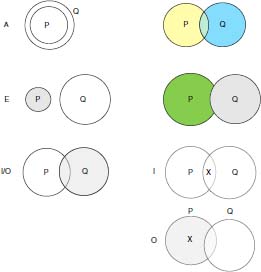
The last syllogism of example 2.12:

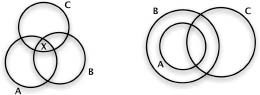
The syllogism:

No A is a B

Every C is an A

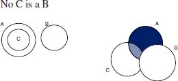
We first recall the definitions that permit us to characterize PL using algebra.

Usually, lattices are defined in two separate ways: one as an algebraic structure and the other based on orderings.

DEFINITION 3.22.– (Boolean algebra). A Boolean algebra is an algebra (see definition 5.4), that is a lattice (T1-T4), which is distributive (T5), bounded (T6), and with complements (T7):

(the operations ∨ and ∧ are, respectively, called join and meet.

and for all x, y, z in T (T non-empty, see definition 5.4)

T1)

T2)

T3)

T4)

T5)

T6)

T7)

EXAMPLE 3.17.– (set theory, Boolean algebra and PL). Let U denote a set (universe). The algebra:

where:

(U): set of subsets of U

is a Boolean algebra.

The well-known relationship between (operators of) set theory and connectives in PL is given in the following table:

More generally, every Boolean algebra is isomorphic to a non-empty family (of subsets of a set) that is closed for the union, intersection, and complement operations²¹.

Before giving the definition of a lattice based on the notion of orderings, we recall the definitions of a partial order, sup, and inf.

DEFINITION 3.23.– (order).

– A partially ordered set or poset is a set A ≠ ∅ and a binary relation that satisfies, for all x, y, z in A:

if furthermore:

then is a total order and is a totally ordered set or chain.

(OP1), (OP2), and (OP3) define an order relation and (OP1), (OP2), (OP3), and (OP4) a total order relation.

– Let denote a poset and H ⊆ A, a ∈ A is an upper bound of H iff for all . If for all upper bounds b, , then a is called the supremum (or least upper bound), denoted by sup. The supremum is unique.

Similarly, we define the infimum (greatest lower bound), which is unique and denoted by inf.

We define iff and x ≠ y.

Similarly, we define iff or x = y.

An equivalent definition of partially ordered sets follows.

DEFINITION 3.24.– (order-bis).

– A partially ordered set or poset is a set A ≠ ∅ together with a binary relation satisfying, for all x, y, z in A:

Note that (OP1') and (OP3') are sufficient to axiomatize an order (see exercise 5.3 d)).

A total order is often defined as follows:

DEFINITION 3.25.– (total order-bis).

– A totally ordered set, is a set A ≠ ∅ together with a binary relation satisfying, for all x, y, z in A:

THEOREM 3.6.– A poset is a lattice if sup {a, b} and inf {a, b} exist for all a, b ∈ A.

(We define a ∨ b :^def sup {a, b}; a ∧ b :^def inf {a,b})

EXAMPLE 3.18.– The algebra:

with ∨, ∧, ¬ defined in definition 3.6 (with 0: F, 1: T and, as in ) is a Boolean algebra (the simplest one).

DEFINITION 3.26.– (congruence, quotient algebra). An equivalence relation (i.e. a reflexive, symmetric, and transitive relation) ~ in an algebra < ; > is a congruence relation iff for all the operations denoted by the function symbols

if a₁ ~ b₁, a₂ ~ b₂, …, a_n ~ b_n; a_i, b_i ∈ A(1 ≤ i ≤ n), then f⁽ⁿ⁾ (a₁, a₂, …, a_n) ~ f⁽ⁿ⁾ (b₁, b₂, …, b_n).

The equivalence classes are denoted by | a_i |.

We can define the operations on the partition induced by ~ (denoted by A/~):

The algebra:

is called the quotient algebra.

If we consider the language ₀ and we define the binary relation ~:

for all

~ is an equivalence relation.

The equivalence classes thus defined represent the formal definition of a proposition (see also exercise 3.6).

By defining:

the algebra:

is a Boolean algebra, called the Lindenbaum algebra of PL.

---

1 The term clause is also used in the simplification of truth functions and test of their validity, to designate the disjuncts of a dnf, that is, the conjunction of literals (see remark 3.36).

2 Strictly speaking, we should make the value of I on ∏{A, B, C, D, E, F} explicit or clarify that it is an interpretation of the formula .

3 Irreflexivity non-reflexive .

4 The Greeks invented democracy at the same time.

5 Rhetoric was part of the French official education program until the 19th Century. There was a renewed interest in rhetoric during the 20th Century.

6 Dialectic comes from a verb meaning to discuss.

7 See below the characteristics of a proof when answering the question “What is a proof?”

8 Here, the author’s requirements coincide with those that form the basis of proof theory.

9 Of course, this requirement also holds for other human activities: a writer noticed that since 1922 and until the correct edition, more than 5,000 printing errors had been made in Joyce’s Ulysses. Because the book was believed to be incomprehensible, no one had noticed the mistakes.

10 There should be a special mention to probabilistic proofs and zero-knowledge proofs. In the former, random verifications with negligible possible errors can be carried out. In the latter, someone who does not know of a proof produced elsewhere can be convinced of the correctness of a result without knowing how it was obtained.

11 This is clearly related to the idea behind proof assistants and logical frameworks.

12 There exists a mathematical journal named Experimental Mathematics.

13 The author forgot that there were many wrong “proofs” (obtained by excellent mathematicians), like those mentioned in the four-color theorem, well before computers ever existed.

14 See also digressions 5.2 and 9.1.

15 From the Latin word meaning “thing that follows”

16 Although Hilbert did not specify what he meant by “finitist”, all finitary methods can probably be formulated in the ZFC formalization (ZF + AC) in set theory.

17 There also exists a non-clausal resolution.

18 The dual of the expression V(x,y, …, z) is defined as ¬(Λ(¬x, ¬y,..., ¬z)), where x, y, …, z are literals.

19 Important works have been carried out on this topic, in particular, by Gödel on second-order logic compared with first-order logic.

20 Necessarily, as n is fixed but unknown.

21 When U is finite, this notion corresponds to that of finite probability spaces.