
CIRCUMFERENCE AND AREA OF AN ELLIPSE
When you draw an ellipse (or use the 3D printed model) you can also find the
circumference, the distance all the way around it. (Sometimes people use the
word perimeter for the distance all the way around anything but a circle, so
you may see that too.) Lay down a piece of string around the ellipse, mark off
the circumference on the string, and then straighten out the string on a ruler
to measure the circumference. Bizarrely, there is no simple equation for the
circumference of an ellipse, for reasons that need to wait until you’ve had
calculus. Around 1914, the Indian mathematician Srinivasa Ramanujan came
up with this approximation (a squiggly equals sign means “approximately”):
Circumference of an ellipse
͌
π [3(a+b)- √
(3a+b) (a+3b)
]
It is a tribute to how hard this problem is that this approximation is only
about 100 years old. Ramanujan, who lived in British India during its colonial
period, did not have any formal training in higher mathematics but came up
with this and other innovations largely on his own. He also developed better,
more complex approximations as well; search on his name and “ellipse cir-
cumference” (sometimes called “ellipse perimeter”) for more. Unfortunately,
he died at age 32, or who knows how many other simplifications he would
have come up with. The full solution involves an advanced calculus equation
called an “elliptic integral”, but this should serve you well for now.
The area of an ellipse is more straightforward. It is:
Area = πab
To demonstrate it to yourself, consider that as an ellipse gets more and more
like a circle, both a and b become a radius. So πab would become the more
familiar πr.
ORBITS OF PLANETS AND KEPLER’S LAWS
For thousands of years, people believed that all the planets revolved around
the Earth. They had to make up all sorts of weird explanations for the fact
that planets seem to sometimes move one way on the sky, and sometimes
another. In 1543, the Polish mathematician Nicholas Copernicus explained
that the planets moved in circles around the sun. In the early 1600s German
mathematician Johannes Kepler figured out that if he modeled the planets’
orbits as ellipses with the sun at one focus rather than as circles, the Coper-
nican model was even better at predicting the motion of the planets in the
Make: Geometry 223
Geometry_Chapter10_v15.indd 223Geometry_Chapter10_v15.indd 223 6/23/2021 9:11:01 AM6/23/2021 9:11:01 AM

sky.
Kepler organized his theory of how planets moved
into three laws:
1. Planets orbit the sun in an elliptical orbit,
with the sun at one focus.
2. A line dragged from the sun to a planet
would sweep out an equal area of its orbit
during an equal time (Figure 11-8). By
“sweeping out”, we mean if you imagine
a string from the planet to the sun, as
the planet moved around the cord would
stretch (or contract) and drag along the
imaginary plane of the orbit, creating the
colored areas in Figure 11-8.
3. The square of the period of an orbit (the
time it takes a planet to go around once) is
proportional to the cube of the semimajor
axis of its orbit.
His laws, based largely on many careful observa-
tions by the astronomer Tycho Brahe, explained a
lot. For example, planets closer to the sun, by the
second law, have to move faster to sweep out the
same area as a planet with a larger orbital radius.
Kepler didn’t know about moons around planets,
or planets around other stars. (Later astrono-
mers would need to generalize his laws to allow
for the gravitational pull of the bodies orbiting and
some other factors.) Soon after, though, Galileo
saw the moons of Jupiter through a telescope and
corresponded with Kepler about it. It took a while,
but eventually this view of how the solar system
worked was accepted.
Figures 11-9 and 11-10 show a set of 3D printed
models of Kepler’s laws described in our book, 3D
Printed Science Projects (Apress, 2016). The base
is an orbit, with the foci marked, and the height
is the speed at that point in the orbit. Figure 11-9
shows the orbit of Halley’s Comet, which has an
FIGURE 118: Sweeping out areas of an ellipse
FIGURE 1110: Orbits of Earth, Venus, and Mercury (mutually
to scale, but not to the same scale as Figure 11-9).
FIGURE 119: The orbit of Halley’s Comet
Make: Geometry 225
224 Chapter 11: Constructing Conics
Geometry_Chapter10_v15.indd 224Geometry_Chapter10_v15.indd 224 6/23/2021 9:11:03 AM6/23/2021 9:11:03 AM

orbit that is a long, skinny ellipse with the sun at
a focus way out near the end of the semimajor
axis. In the 3D print, the foci are pretty much
buried in the wall at each end of the ellipse.
Figure 11-10 shows the orbits and orbital veloc-
ities of Mercury, Venus, and Earth (to scale with
each other, but not to Halley’s Comet).
As you can see from the height of the model,
the comet is moving very fast near the sun, then
slows to a crawl at the other extreme as it moves
along in its 75-year-long orbit. Mercury, too, has
a somewhat elliptical orbit and will go faster in
the part of its orbit nearer the sun than it will in
the other. Looking at the set of three orbits, as
we go farther from the sun, the orbits of Venus
and Earth are each slower than the planets
closer to the sun.
This variation of the speed of a planet, like Earth,
in its trip around the sun is a major component
in the Equation of Time. We learned about the
Equation of Time in Chapter 7 when we had to
look up its value to deduce our location based
on when the sun was highest in the sky. Earth’s
orbit is very nearly circular, but even that small
difference matters. In Chapter 12, we will reprise
that, and go into more depth about how to take
these effects into account when using the sun to
tell time.
PARABOLA
As we saw in Chapter 10, a parabola is created
only when a cutting plane is exactly parallel to
the slant angle of the cone. If the cutting plane is
any shallower (relative to the bottom of the cone) you get an ellipse; any steeper, you get a hyperbola.
A parabola can be thought of as the special case where an ellipse transitions into a hyperbola. It is
shaped somewhere between the letters U and V (never quite coming to an actual point). The sharpest
point of its turnaround is called the vertex. Some people like to think of a hyperbola as an inside-out
ellipse. After we talk about all three, we’ll come back to that.
Directrix and Generatrix
Getting further into the details of conic sections
requires that we make the acquaintance of a new
pair of abstract ideas, the directrix and generatrix
(sometimes called a generator instead). Despite
sounding like pets of superheroes, they are imag-
inary tools that can help us draw a curve. Since
we are all about being hands-on, we are going to
make and use physical versions in the next sec-
tions of this chapter.
A generatrix is a point, curve, or surface that
when moved along a certain path carves out a
desired line, surface, or 3D shape, respectively. A
directrix is that path.
For example, take a straight line that has the
top end pinned at a point and the bottom swept
around a circle to sweep out a cone. The line is
the generatrix, and the circle is the directrix. We
are going to use a directrix to construct conic
sections (specifically, hyperbolas and parabolas)
without (much) algebra, in case you want to make
something physical in one of these shapes. You
know how to make an ellipse now (with a pinned
string or rope). Let’s see how to draw parabolas
and hyperbolas, and why you might want to.
Make: Geometry 225
Geometry_Chapter10_v15.indd 225Geometry_Chapter10_v15.indd 225 6/23/2021 9:11:03 AM6/23/2021 9:11:03 AM
After reading the last section, you probably won’t be surprised to know that a parabola can be defined in
terms of a focus, but only one. An alternative way to think about it is to imagine the ellipse we get from
slicing a cone. As the cut gets steeper, the ellipse gets larger, and the major axis gets larger faster than
the minor axis. When the cut is parallel to the side of the cone, the ellipse would never cross the side of
the cone to close the ellipse. We can imagine that one focus has slid out to infinity. Our trick of using two
foci we used to draw the ellipse won’t work here, but we can do something almost as simple.
DRAWING A PARABOLA
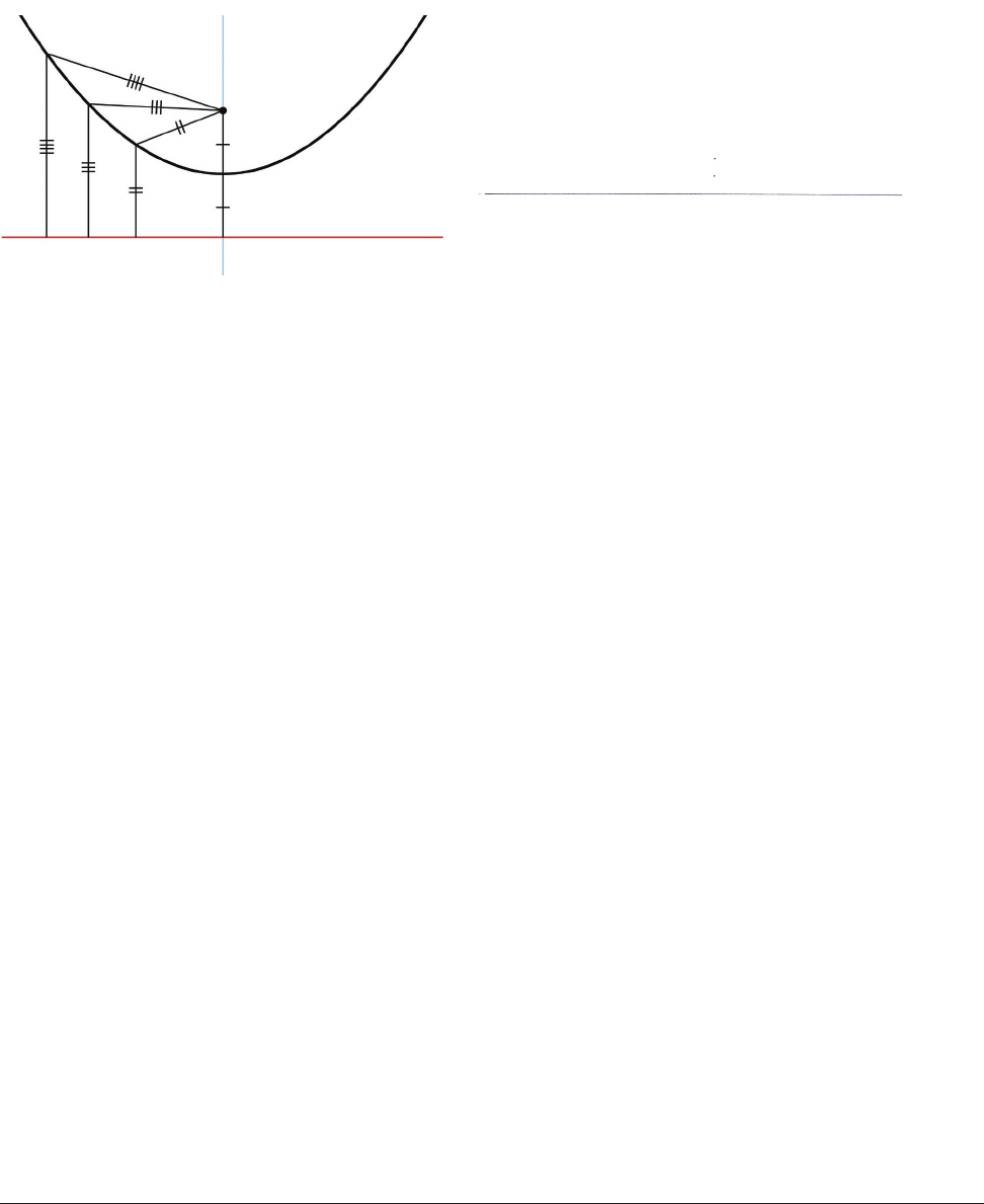
In addition to its conic section definition, a parabola can also be described as a curve that has every
point an equal distance from a point (the focus) and the shortest distance to a line (the directrix). In
Figure 11-11, we show these distances marked with little hash marks. Lines with one hash mark are
equal in length to each other, the ones with two are equal to each other, and so on. The directrix is
shown in red.
In the “Directrix and Generatrix” sidebar we get into this a little more, but, briefly, once you pick your
directrix and focus, your parabola has been completely specified. Just like cutting a cone parallel to its
side, picking a directrix and focus is a means of generating a parabola geometrically. A parabola can
open at any angle. The parabola will always open away from the directrix, with the focus on its center-
line. If the directrix is above a focus, then the parabola will open downward, and if the directrix is below
the focus, the parabola will open upward.
The lowest point of the parabola in Figure 11-11 is called its vertex. It lies along a line (shown in blue in
Figure 11-11) that is perpendicular to the directrix and goes through the focus. The focus and directrix
are equal distances from the vertex, and this is the closest the curve approaches to either.
We’ve created a 3D printed model, centerfinders.scad, which allows you to play with these concepts.
We can use it to create both hyperbolas and parabolas. It’s the equivalent of what we did with the push
pins and string for an ellipse. Here is how it works.
If we want to draw a parabola, we have to find a series of points that are the same distance from the
FIGURE 1111: A parabola, showing its directrix line (red),
focus, and lines of equal distance
FIGURE 1112: Finding the vertex of the parabola (lower dot)
from focus (upper dot) and directrix (line)
Make: Geometry 227
226 Chapter 11: Constructing Conics
Geometry_Chapter10_v15.indd 226Geometry_Chapter10_v15.indd 226 6/23/2021 9:11:05 AM6/23/2021 9:11:05 AM
focus and the directrix line. One way to do that is to draw a series of circles
that each just touch the focus and the directrix, since a circle centered on one
point of the parabola will have the focus and directrix both touch its perime-
ter somewhere. However, it’s tough to draw a circle if you don’t know where
the center is (since that is the point we are trying to find).
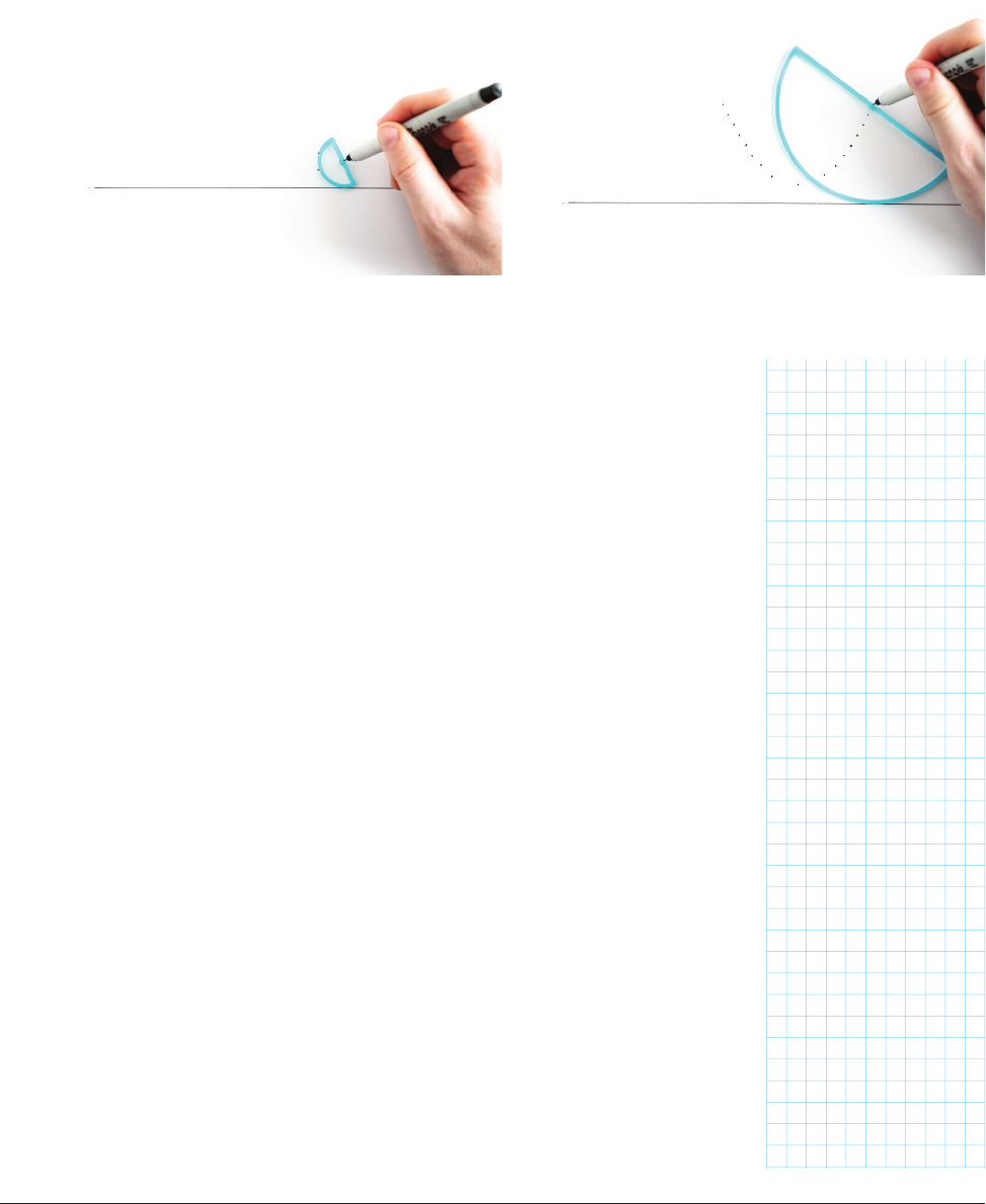
The centerfinders.scad model prints out a series of shapes that look like a
capital letter “D”. To draw a parabola, first draw a directrix and a focus. Find
the spot midway between the focus and the directrix with a ruler; that will be
the vertex of the parabola (Figure 11-12).
Then take the smallest D and just touch the directrix and focus with the outer
part (Figure 11-13). Make a dot in the notch on the flat point. That is the next
point of the parabola.
Then, take the next-biggest D and so on. Note that each D can make two
points - one on each side of the vertex, since a parabola is symmetrical
(Figure 11-14).
Once you have this series of points, you can sketch in the final parabola
between them (Figure 11-15).
If you want to adapt centerfinders.scad a bit, you can change how many
D-shaped pieces you make, how large they are, and how different the size is
from one to the next by changing the radii set of three variables.
The default is: radii = [10:6:60];
This, as we saw in Chapter 2, means that the smallest radius piece will have
FIGURE 1113: Starting the parabola FIGURE 1114: The parabola has two symmetrical points on
either side of its vertex.
Make: Geometry 227
Geometry_Chapter10_v15.indd 227Geometry_Chapter10_v15.indd 227 6/23/2021 9:11:08 AM6/23/2021 9:11:08 AM
..................Content has been hidden....................
You can't read the all page of ebook, please click here login for view all page.