7

Advanced Clustering and Unsupervised Models

In this chapter, we will continue to analyze clustering algorithms, focusing our attention on more complex models that can solve problems where K-means fails. These algorithms are extremely helpful in specific contexts (for example, geographical segmentation) where the structure of the data is highly non-linear and any approximation leads to a substantial drop in performance.

In particular, the algorithms and the topics we are going to analyze are:

• Fuzzy C-means
• Spectral clustering based on the Shi-Malik algorithm
• DBSCAN, including the Calinski-Harabasz and Davies-Bouldin scores

The first model is Fuzzy C-means, which is an extension of K-means to a soft-labeling scenario. Just like Generative Gaussian Mixtures, the algorithm helps the data scientist to understand the pseudo-probability (a measure similar to an actual probability) of a data point belonging to all defined clusters.

Fuzzy C-means

We have already talked about the difference between hard and soft clustering, comparing K-means with Gaussian mixtures. Another way to address this problem is based on the concept of fuzzy logic, which was proposed for the first time by Lotfi Zadeh in 1965 (for further details, a very good reference is Pedrycz W., Gomide F., An Introduction to Fuzzy Sets, The MIT Press, 1998). Classic logic sets are based on the law of excluded middle, which in a clustering scenario can be expressed by saying that a point can belong only to a single cluster c_j.

Speaking more generally, if we split our universe into labeled partitions, a hard clustering approach would assign a label to each sample, while a fuzzy (or soft) approach would allow the management of a membership degree (in Gaussian mixtures, this is an actual probability) w_ij, which expresses how strong the relationship is between point and cluster c_j.

Contrary to other methods, by employing fuzzy logic it's possible to define asymmetric sets that are not representable with continuous functions (such as trapezoids). This allows further flexibility and an increased ability to adapt to more complex geometries. The following graph shows examples of fuzzy sets:

Examples of fuzzy sets representing the seniority level of an employee according to years of experience

The graph represents the seniority level of an employee given their years of experience. As we want to cluster the entire population into three groups (Junior, Middle, and Senior level employees), three fuzzy sets have been designed. We have assumed that a young employee is keen and can quickly reach the Junior level after an initial apprenticeship period. The opportunity to work on complex problems allows them to develop skills that are fundamental to the transition between the Junior and Middle levels. After about 10 years, the employee can begin to consider themselves as a Senior apprentice and, after about 25 years, their experience is enough to qualify them as a full Senior until the end of their career.

As this is an imaginary example, we haven't tuned all of the values, but it's easy to compare, for example, employee A who has 7 years of experience with employee B who has 18 years of experience. The former is about 25% Junior (decreasing even if with a minimum slope), 25% Middle (reaching its climax), and almost 0% Senior (increasing). The latter is 0% Junior (ending plateau), about 0% Middle (decreasing), and close to 100% Senior (ending plateau).

In both cases, the values are not normalized so always sum up to 1 because we are more interested in showing the process and the proportions. The fuzziness level is lower in extreme cases, while it is higher when two sets intersect. For example, at about 15%, the Middle and Senior are about 50%. As we're going to discuss, it's useful to avoid a very high fuzziness level when clustering a dataset because it can lead to a lack of precision as the boundaries fade out, becoming completely fuzzy.

Fuzzy C-means is a generalization of standard K-means, with a soft assignment and more flexible clusters. The dataset to cluster (containing M samples) is represented by:

If we assume we have k clusters, it's necessary to define a matrix containing the membership degrees for each sample:

Each degree and all rows must be normalized so that they always sum up to 1. In this way, the membership degrees can be considered as probabilities (with the same semantics) and it's easier to make decisions with a prediction result. If a hard assignment is needed, it's possible to employ the same approach normally used with Gaussian mixtures: the winning cluster is selected by applying the argmax function. However, it's good practice to employ soft clustering only when it's possible to manage the vectorial output. For example, the probabilities/membership degrees can be fed into a classifier in order to yield more complex predictions.

As with K-means, the problem can be expressed as the minimization of generalized inertia:

The constant m (m > 1) is an exponent employed to re-weight the membership degrees. A value very close to 1 doesn't affect the actual values. Greater m values reduce their magnitude. The same parameter is also used when recomputing the centroids and the new membership degrees and can lead to a different clustering result. It's rather difficult to define a globally acceptable value; therefore, a good practice is to start with an average m (for example, 1.5) and perform a grid search (it's possible to sample from a Gaussian or uniform distribution) until the desired accuracy has been achieved.

Minimizing the previous expression is even more difficult than with standard inertia; therefore, a pseudo-Lloyd's algorithm is employed. After a random initialization, the algorithm proceeds, alternating two steps (like an EM procedure) in order to determine the centroids and recomputing the membership degrees to maximize the internal cohesion. The centroids are determined by a weighted average:

Contrary to K-means, the sum is not limited to the points belonging to a specific cluster because the weight factor will force the farthest points () to produce a contribution close to 0. At the same time, as this is a soft-clustering algorithm, no exclusions are imposed, to allow a sample to belong to any number of clusters with different membership degrees. Once the centroids have been recomputed, the membership degrees must be updated using this formula:

This function behaves like a similarity. In fact, when sample x_i is very close to centroid (and relatively far from with ), the denominator becomes small and w_ij increases. The exponent m directly influences the fuzzy partitioning, because when (m > 1), the denominator is a sum of quasi-squared terms and the closest centroid can dominate the sum, yielding to a higher preference for a specific cluster. When m >> 1, all the terms in the sum tend to 1, producing a flatter weight distribution with no well-defined preference.

It's important to understand that, even when working with soft clustering, a fuzziness excess leads to inaccurate decisions because there are no factors that push a sample to clearly belong to a specific cluster. This means that the problem is either ill-posed or, for example, the number of expected clusters is too high and doesn't represent the real underlying data structure. A good way to measure how much this algorithm is similar to a hard-clustering approach (such as K-means) is provided by the normalized Dunn's partitioning coefficient:

When P_C is bounded between 0 and 1, when it's close to 0, it means that the membership degrees have a flat distribution and the level of fuzziness is the highest possible. On the other hand, if it's close to 1, each row of W has a single dominant value, while all the others are negligible. This scenario resembles a hard-clustering approach. Larger P_C values are normally preferable because, even without allowing a degree of fuzziness, they allow the making of more precise decisions.

Considering the previous example, P_C tends to 1 when the sets don't intersect, while it becomes 0 (complete fuzziness) if, for example, the three seniority levels are chosen to be identical and overlapping. Of course, we are interested in avoiding such extreme scenarios by limiting the number of borderline cases. A grid search can be performed by analyzing different numbers of clusters and m values (in the example, we're going to do this with the MNIST handwritten digit dataset). A reasonable rule of thumb is to accept P_C values higher than 0.8, but in some cases that can be impossible. If we are sure that the problem is well-posed, the best approach is to choose the configuration that maximizes P_C, considering, however, that a final value of less than 0.3 - 0.5 will lead to a very high level of uncertainty because the clusters will overlap extremely.

The complete Fuzzy C-means algorithm is:

1. Set a maximum number of iterations N_max
2. Set a tolerance Thr
3. Set the value of k (the number of expected clusters)
4. Initialize the matrix W⁽⁰⁾ with random values and normalize each row, dividing it by its sum
5. Set N = 0
6. While or :
   1. N = N +1
   2. For j = 1 to k:
      1. Compute the centroid vectors
   3. Recompute the weight matrix W^(t)
   4. Normalize the rows of W^(t)

After the theoretical discussion, we can now analyze a concrete example of this algorithm using the scikit-fuzzy Python package, comparing the results with a classical hard-clustering approach.

Example of Fuzzy C-means with SciKit-Fuzzy

SciKit-Fuzzy (http://pythonhosted.org/scikit-fuzzy/) is a Python package based on SciPy (it can be installed using the pip install -U scikit-fuzzy command. For further instructions, please visit http://pythonhosted.org/scikit-fuzzy/install.html, which allows you to implement all the most important fuzzy logic algorithms (including fuzzy C-means).

In this example, we'll continue to use the MNIST dataset we used in the previous chapter, but with a major focus on fuzzy partitioning. To perform the clustering, SciKit-Fuzzy implements the cmeans method (in the skfuzzy.cluster package), which requires a few mandatory parameters: data, which must be an array (N is the number of features; therefore, the array used with scikit-learn must be transposed); c, the number of clusters; the coefficient m, error, which is the maximum tolerance; and maxiter, which is the maximum number of iterations. Another useful parameter (not mandatory) is the seed parameter, which allows you to specify the random seed to be able to easily reproduce the experiments. I invite you to check the official documentation for further information.

The first step of this example is performing the clustering:

from skfuzzy.cluster import cmeans
fc, W, _, _, _, _, pc = 
    cmeans(X_train.T, c=10, m=1.25, 
           error=1e-6, maxiter=10000, seed=1000)

The cmeans function returns many values, but for our purposes, the most important are: the first one, which is the array containing the cluster centroids; the second one, which is the final membership degree matrix; and the last one, the partition coefficient. In order to analyze the result, we can start with the partition coefficient:

print('Partition coeffiecient: {}'.format(pc))

The output is:

Partition coeffiecient: 0.6320708707346328

This value informs us that the clustering is not very far from a hard assignment, but there's still a residual fuzziness. In this particular case, such a situation may be reasonable because we know that many digit images are partially distorted, and may appear very similar to other digits (1, 7, and 9 are easily confused). However, I invite you to try different values for m and check how the partition coefficient changes. We can now display the centroids:

Centroids obtained by Fuzzy C-Means

All the different digit classes have been successfully found, but now, contrary to K-means, we can check the fuzziness of a problematic sample (representing a 7 with index 7), as shown in the following figure:

Sample (a 7) selected to test the fuzziness

The membership degrees associated with the previous sample are:

print('Membership degrees: {}'.format(W[:, 7]))

The output is:

Membership degrees: [0.00373221 0.01850326 0.00361638 
                     0.01032591 0.86078292 0.02926149
                     0.03983662 0.00779066 0.01432076 
                     0.0118298]

The corresponding plot is:

Fuzzy membership plot corresponding to a digit representing a 7

In this case, the choice of m has forced the algorithm to reduce the fuzziness. However, it's still possible to see three smaller peaks corresponding to the clusters centered respectively on the digits 1, 8, and 3 (remember that the cluster indexes – 1, 6, and 8, in this case – correspond to digits shown previously in the centroid plot). I invite you to analyze the fuzzy partitioning of different digits and replot it with different values of the m parameter. It will be possible to observe an increased level of fuzziness (also corresponding to smaller partitioning coefficients) with larger m values. This effect is due to a stronger overlap among clusters (also observable by plotting the centroids) and could be useful when it's necessary to detect the distortion of a sample. In fact, even if the main peak indicates the right cluster, the secondary ones, in descending order, inform us how much the sample is similar to other centroids and, therefore, if it contains features that are characteristics of other subsets.

Contrary to scikit-learn, in order to perform predictions, SciKit-Fuzzy implements the cmeans_predict method (in the same package), which requires the same parameters as cmeans, but instead of the number of clusters, c needs the final centroid array (the name of the parameter is cntr_trained). The function returns as a first value the corresponding membership degree matrix (the other ones are the same as cmeans). In the following snippet, we repeat the prediction for the same sample digit (representing a 7):

import numpy as np
from skfuzzy.cluster import cmeans_predict
new_sample = np.expand_dims(X_train[7], axis=1)
Wn, _, _, _, _, _ = 
    cmeans_predict(new_sample, cntr_trained=fc, m=1.25, 
                   error=1e-6, maxiter=10000, seed=1000)
print('Membership degrees: {}'.format(Wn.T))

The output is:

Membership degrees: [[0.00373221 0.01850326 0.00361638 
                      0.01032591 0.86078292 0.02926149
                      0.03983662 0.00779066 0.01432076 
                      0.0118298]]

Spectral clustering

One of the most common problems with K-means and other similar algorithms is the assumption that we only have hyperspherical clusters. In fact, K-means is insensitive to the angle and assigns a label only according to the closest distance between a point and centroids. The resulting geometry is based on hyperspheres where all points share the same condition to be closer to the same centroid. This condition might be acceptable when the dataset is split into blobs that can be easily embedded into a regular geometric structure. However, it fails whenever the sets are not separable using regular shapes. Let's consider, for example, the following bidimensional dataset:

Sinusoidal dataset

As we are going to see in the example, any attempt to separate the upper sinusoid from the lower one using K-means will fail. The reason is obvious: a circle that contains the upper set will also contain part of the (or the whole) lower set. Considering the criterion adopted by K-means and imposing two clusters, the inertia will be minimized by a vertical separation corresponding to about x₀ = 0. Therefore, the resulting clusters are completely mixed and only a dimension is contributing to the final configuration. However, the two sinusoidal sets are well-separated and it's not difficult to check that, selecting a point x_i from the lower set, it's always possible to find a ball containing only samples belonging to the same set. We discussed this kind of problem when Label Propagation algorithms were discussed and the logic behind spectral clustering is essentially the same (for further details, I invite you to check out Chapter 5, Graph-Based Semi-Supervised Learning).

Let's suppose we have a dataset X sampled from a data generating process p_data:

We can build a graph G = {V, E}, where the vertices are the points and the edges are determined using an affinity matrix W. Each element w_ij must express the affinity between the points and . W is normally built using two different approaches:

• K-Nearest Neighbor (KNN): In this case, we can build the number of neighbors to take into account for each point . W can be built as a connectivity matrix (expressing only the existence of a connection between two samples) if we adopt the criterion:

Alternatively, it's possible to build a distance matrix:

• Radial basis function (RBF): The previous methods can lead to graphs that are not fully connected because samples can exist that have no neighbors. In order to obtain a fully connected graph, it's possible to employ an RBF (this approach has also been used in the Kohonen map algorithm, discussed in Chapter 15, Fundamentals of Ensemble Learning):

The parameter allows you to control the amplitude of the Gaussian function, reducing or increasing the number of samples with a large weight (actual neighbors). However, a weight is assigned to all points and the resulting graph will always be connected (even if many elements are close to zero).

In both cases, the elements of W will represent a measure of affinity (or closeness) between points and no restrictions are imposed on the global geometry (contrary to K-means). In particular, using a KNN connectivity matrix, we are implicitly segmenting the original dataset into smaller regions with a high level of internal cohesion. The problem that we need to solve now is to find out a way to merge all the regions belonging to the same cluster.

The approach we are going to present here has been proposed by Shi and Malik (in Shi J., Malik J., Normalized Cuts and Image Segmentation, IEEE Transactions on Pattern Analysis and Machine Intelligence, Vol. 22, 08, 2000), and it's based on the normalized graph Laplacian:

The matrix D, called the degree matrix, is the same as was discussed in Chapter 5, Graph-Based Semi-Supervised Learning, and it's defined as:

It's possible to prove the following properties (the formal proofs are omitted but they can be found in texts such as Gelfand I. M., Glagoleva E. G., Shnol E. E., Functions and Graphs Vol. 2, The MIT Press, 1969 or Biyikoglu T., Leydold J., Stadler P. F., Laplacian Eigenvectors of Graphs, Springer, 2007):

• The eigenvalues and the eigenvectors of L_n can be found by solving the problem , where L is the unnormalized graph Laplacian L = D - W
• L_n always has an eigenvalue equal to 0 (with a multiplicity k) with a corresponding eigenvector
• As G is undirected and all , the number of connected components k of G is equal to the multiplicity of the null eigenvalue

In other words, the normalized graph Laplacian encodes the information about the number of connected components and provides us with a new reference system where the clusters can be separated using regular geometric shapes (normally hyperspheres). To better understand how this approach works without a non-trivial mathematical approach, it's important to expose another property of L_n.

From linear algebra, we know that each eigenvalue of a matrix spans a corresponding eigenspace, which is a subset of containing all eigenvectors associated with plus the null vector. Moreover, given a set and a countable subset C (it's possible to extend the definition to generic subsets but in our context, the datasets are always countable), we can define a vector as an indicator vector, if if the vector and otherwise. If we consider the null eigenvalues of L_n and we assume that their number is k (corresponding to the multiplicity of the eigenvalue 0), it's possible to prove that the corresponding eigenvectors are indicator vectors for eigenspaces spanned by each of them.

From the previous statements, we know that these eigenspaces correspond to the connected components of the graph G; therefore, performing standard clustering (like K-means or K-means++) with the points projected into these subspaces allows easy separation with symmetric shapes.

Since , its eigenvectors . Selecting the first k eigenvectors, it's possible to build a matrix :

Each row of A, , can be considered as the projection of an original point in the low-dimensional subspace spanned by the eigenvectors associated with the null eigenvalues of L_n. At this point, the separability of the new dataset depends only on the structure of the graph G and, in particular, on the number of neighbors or the parameter for RBFs. As in many other similar cases, it's impossible to define a standard value suitable for all problems, above all when the dimensionality doesn't allow a visual inspection. A reasonable approach should start with a small number of neighbors (for example, 5 or 10) or and increase the values until a performance metric (such as the Adjusted Rand Index) reaches its maximum.

Unfortunately, every problem has very specific requirements and it's quite difficult to provide the data scientist with rock-solid default values. All toolkits tend to use intermediate parameter levels, letting the user choose the most appropriate configuration. Considering a KNN scenario, for example, 5, 10, or 100 neighbors could be a reasonable choice if the underlying topology is compatible. It must be clear that a neighborhood should always be relatively small. More precisely, the user can imagine the neighborhood of a point as a building block (indeed, they are employed as bases in topology theory) to construct the overall hypersurface (or manifold) where the dataset lies. Given a metric function, the minimum number of neighbors can be determined considering the sample size S. Values corresponding to 0.1% - 0.5% of S could be good default choices when the density is large enough. On the other hand, excessive granularity might also yield incorrect results due to the large number of connected components.

Another important element to remember is that KNN often leads to non-connected affinity matrices. All the most common libraries can manage numeric instability problems (for example, if the degree matrix has det(D) = 0, it's not invertible and more robust solutions must be employed), but in some particular cases, split graphs could hide relevant information about the structure.

Therefore, you should carefully evaluate the strategy to compute W and check the results when the software outputs warnings about the lack of connectivity (for example, scikit-learn outputs a precise warning, which must always be taken into account).

Considering the nature of the problems, it can also be helpful to measure homogeneity and completeness (discussed in the previous chapter) because these two measures are more sensitive to irregular geometric structures and can easily show when the clustering is not separating the sets correctly. If the ground truth is unknown, the Silhouette score can be employed to assess the intra-cluster cohesion and the inter-cluster separation as functions of all hyperparameters (the number of clusters, the number of neighbors, or ).

The complete Shi-Malik spectral clustering algorithm is:

1. Select a graph construction method between KNN (1) and RBF (2):
   1. Select parameter k
   2. Select parameter
2. Select the expected number of clusters N_K
3. Compute the matrices W and D
4. Compute the normalized graph Laplacian L_n
5. Compute the first k eigenvectors of L_n
6. Build the matrix A
   1. Cluster the rows of A using K-means++ (or any other symmetric algorithm).

The output of this process is this set of clusters: At this point, we can create an example using scikit-learn with the goal being to compare the performances of K-means with spectral clustering.

Example of spectral clustering with scikit-learn

In this example, we are going to use the sinusoidal dataset previously shown. The first step is creating it (with 1,000 samples):

import numpy as np
from sklearn.preprocessing import StandardScaler
nb_samples = 1000
X = np.zeros(shape=(nb_samples, 2))
for i in range(nb_samples):
    X[i, 0] = float(i)
    
    if i % 2 == 0:
        X[i, 1] = 1.0 + (np.random.uniform(0.65, 1.0) * 
                         np.sin(float(i) / 100.0))
    else:
        X[i, 1] = 0.1 + (np.random.uniform(0.5, 0.85) * 
                         np.sin(float(i) / 100.0))
        
ss = StandardScaler()
Xs = ss.fit_transform(X)

At this point, we can try to cluster it using K-means (with n_clusters=2):

from sklearn.cluster import KMeans
km = KMeans(n_clusters=2, random_state=1000)
Y_km = km.fit_predict(Xs)

The result is shown in the following graph:

K-means clustering result using the sinusoidal dataset

As expected, K-means isn't able to separate the two sinusoids. You're free to try with different parameters, but the result will always be unacceptable because K-means bidimensional clusters are circles (when working in they become hyperspheres, but the structural relations remain the same) and no valid configurations exist. It's easy to understand that both completeness and homogeneity are very low because each class contains about 50% of the samples of the other one.

We can now employ spectral clustering using an affinity matrix based on the KNN algorithm (in this case, scikit-learn can produce a warning because the graph is not fully connected, but this normally doesn't affect the results). Scikit-learn implements the SpectralClustering class, whose most important parameters are n_clusters, the number of expected clusters; affinity, which can be either rbf or nearest_neighbors; gamma (only for RBF); and n_neighbors (only for KNN). For our test, we have chosen to have 20 neighbors:

from sklearn.cluster import SpectralClustering
sc = SpectralClustering(n_clusters=2, 
                        affinity='nearest_neighbors',
                        n_neighbors=20, 
                        random_state=1000)
Y_sc = sc.fit_predict(Xs)

The result of the spectral clustering is shown in the following figure:

Spectral clustering result using the sinusoidal dataset

As expected, the algorithm was able to separate the two sinusoids perfectly. Even though the scenario is very simple, it perfectly illustrates the advantage of projecting a dataset onto a feature space whenever standard separation is not immediately achievable. The computational cost of computing the kernel is proportionate to the approach (RBF can be faster thanks to the parallelism achievable on modern architectures), but in general, there are no specific limitations except for what's already been discussed about KNN. The main a posteriori consideration with this algorithm concerns its internal structure. Feature spaces and kernels are very powerful tools, but they always require existing regularity in the geometry. In some cases, this is almost impossible to obtain (even using very complex projections) and, consequently, the results might not be extremely accurate.

As an exercise, I invite you to apply spectral clustering to the MNIST dataset, using both an RBF (with different gamma values) and KNN (with different numbers of neighbors). I also suggest replotting the t-SNE diagram and comparing all the assignment errors. As the clusters are strictly non-convex, we don't expect a high Silhouette score. Other useful exercises are drawing the Silhouette plot and checking the result, assigning ground truth labels, and measuring the homogeneity and completeness. Before moving forward, I'd like to remind you that bidimensional plots of high-dimensional datasets must always be carefully evaluated and, above all, obtained through non-linear dimensionality reduction algorithms (for example, t-SNE or LLE). Plotting two features excluding the remaining ones can yield misleading results where, for example, perfectly separated clusters appear as overlapped or vice versa.

In the next section, we are going to discuss an approach that is completely geometry-free and can segment irregular datasets more effectively than other methods.

DBSCAN

Most of the clustering methods discussed so far are based on assumptions about the geometrical structure of the dataset. For example, K-means can find the centroids of hyperspherical regions, while spectral clustering has less limitations (in particular, using a KNN affinity matrix), but it requires you to know the desired number of clusters and such a choice conditions the result. On the other hand, spectral clustering, as well as DBSCAN (which stands for Density-Based Spatial Clustering of Applications with Noise), can work with non-convex clusters, while K-means requires such a condition.

DBSCAN is an algorithm proposed by Ester et al. (in Ester M., Kriegel H. P., Sander J., Xu X., A Density-Based Algorithm for Discovering Clusters in Large Spatial Databases with Noise, Proceedings of the 2nd International Conference on Knowledge Discovery and Data Mining, AAAI Press, pp. 226-231, 1996) to overcome all these limitations.

The main assumption is that X represents a sample drawn from a multimodal distribution, with some dense areas sufficiently separated from one another by almost empty regions. We just said "sufficiently" because DBSCAN also assumes the presence of noisy points that normally lie on the boundaries and could be assigned to more than one cluster. In these cases, algorithms like K-means force the assignment in both possible scenarios:

• . In this case, there is a cluster whose centroid is the closest one and the assignment is straightforward.
• . In this case (which is very unlikely), all distances are equal, therefore the algorithm will normally pick the first cluster (even if the choice could also be perfectly random).

Conversely, DBSCAN, which doesn't require you to specify the desired number of clusters, finds all the topological constraints necessary to separate highly dense and cohesive regions from separation regions. The process works by performing classification on each point, followed by a natural aggregation into labeled clusters and noisy points.

Given a point and a predefined distance metric (for example, Euclidean), the algorithm determines the set of points belonging to the ball . If contains more than n_min points (other than ), is marked as a core point. All other points are marked as directly density-reachable from the core point. A directly density-reachable point has the same importance as a core one, because, from a topological viewpoint, the relation is symmetric (that is, the core point becomes directly density-reachable when the ball is centered on the latter).

Let's now consider a sequence of points . If is directly density-reachable from , the point is marked as density-reachable from .

This concept is weaker than the previous one and it depends both on the radius and on the number n_min. This concept is shown in the following figure:

The point is density-reachable from when

It's easy to verify that is density-reachable from through the sequence when . In fact, with a minimum number of four neighbors, all three points are core ones and each of them is also directly density-reachable from the neighbors, hence, the sequence leads to a density-reachable point.

Given three points , if both and are density-reachable from , they are also marked as density-connected through . Density connection is an even weaker condition and it's not symmetric. In fact, it's possible to find density-connected triplets where is density-reachable from but vice versa doesn't hold. As we move through a sequence in a predefined direction, the connecting point can be directly density-reachable (and, therefore, implicitly a core point) only if its neighborhood contains enough points.

If we denote with the function that counts the number of points belonging to a ball, we can consider a scenario where and , and it's possible to define such that . This allows us to establish a density-reachability condition and we can move forward to the next step involving and . Conversely, when k >> 0, can have less than n_min points, the reachability is broken and we cannot move in the direction . Density connection is a central concept in DBSCAN and most of the work necessary to tune up the hyperparameters concerns the right choice of both and n_min so as to minimize the number of noisy points and to allow the density-connection of all points that must belong to the same cluster. In fact, the algorithm will define a cluster C_p based on:

• All the couples that are density-connected
• If , all that are density-reachable from

After finishing this process, all density-reachable points have been assigned to a cluster. The remaining points, which are formally non-density-reachable by any , are marked as noisy and grouped into an additional virtual cluster.

As anticipated, DBSCAN doesn't require any geometrical constraints but rather relies exclusively on the neighbors of each point. This property guarantees the separability of non-convex regions under the mild assumption that they are separated by low-density hypervolumes (as normally happens). For this reason, DBSCAN is particularly suited to spatial applications with many irregularities (for example, geographical or biomedical segmentation). However, it also works perfectly in many scenarios where simpler algorithms fail. The most important element to consider is its computational complexity, which ranges from to according to the KNN strategy. As the neighbors are normally built using Ball and KD-trees, all considerations discussed in the previous sections are still valid and you should take care when choosing the most appropriate leaf size in order to reduce the number of comparisons and avoid the quadratic complexity (which can be too expensive for large datasets).

Before giving a practical example, it will also be helpful to remind you of the importance of the distance metric chosen for every specific task. When the dataset has high dimensionality, the discriminability of the points can become more difficult using the Minkowski distance with . As DBSCAN relies on the ability of the distance function to discover all density-connected chains, a high-dimensional dataset should be carefully evaluated before choosing the optimal clustering algorithm. Moreover, it's useful to consider the results obtained with the Manhattan distance (which is the most sensitive distance function) and compare them with the ones achieved using the default Euclidean distance. In some cases, the extra discriminability is enough to avoid too many noisy points and to detect most of the density-connected chains. Of course, there are no predefined recipes and the role of the data scientists is also to check the results (using appropriate evaluation metrics such as Calinski-Harabasz or Silhouette score) and validate them together with a business-domain expert.

Example of DBSCAN with scikit-learn

In this example, we are going to build a bidimensional dataset representing a territory where each point is a standardized group of buildings. The goal is to find all the agglomerates and categorize them.

Let's start creating the dataset using 11 partially overlapped bivariate Gaussian distributions:

import numpy as np
mus = [[-5, -3], [-5, 3], [-1, -4], [1, -4], [-2, 0], 
       [0, 1], [4, 2], [6, 4], [5, 1], [6, -3], [-5, 3]]
Xts = []
for mu in mus:
    n = np.random.randint(100, 1000)
    covm = np.diag(np.random.uniform(0.2, 3.5, size=(2, )))
    Xt = np.random.multivariate_normal(mu, covm, 
                                       size=(n, ))
    Xts.append(Xt)
X = np.concatenate(Xts)

A plot of the dataset is shown in the following figure:

Dataset representing a bidimensional spatial distribution of buildings in a geographical area

As it's possible to see, the dataset represents an area where there are some main centers (large agglomerates), secondary ones (smaller agglomerates), and low-density regions (suburbs). Our goal is to employ DBSCAN to find out the optimal number of clusters representing homogeneous areas.

It should be clear that density-connected points make up intrinsically homogeneous regions because of the topological nature of this property (that is, as the balls have a common radius , all density-connected regions have the same average density of all sub-regions). However, as we don't know the ground truth, before starting the analysis, it's helpful to introduce two new evaluation measures: the Calinski-Harabasz and Davies-Boulding scores.

The Calinski-Harabasz score

This score doesn't need the ground truth and evaluates the result of a clustering procedure according to the double principle of maximum cohesion and maximum separation. A reasonable clustering result should show a low variance inside the clusters and a high variance between clusters and separation regions. To quantify this property, we need to introduce two supplementary measures.

Let's suppose that the dataset X has been clustered into k clusters identified by their centroids . The within-cluster-dispersion (WCD) is defined as:

This measure provides a piece of information about the dispersion of the points assigned to each cluster around their respective centroids. In an ideal scenario, this value should be close to its theoretical minimum, indicating that the algorithm has achieved the maximum possible internal cohesion.

If we introduce the function to count the number of points assigned to C_i and the average global centroid (which corresponds to the geometrical center of mass of system containing all ), we can also define the between-cluster-dispersion (BCD):

This measure encodes the separation of the clusters. A large BCD_k indicates that the dense regions are relatively far from each other, where the adjective far means that their centroids aren't near to the global one. Of course, this measure alone isn't helpful, because a cluster can have very large dispersion even when the centroid is far away, as measured by .

Therefore, the Calinski-Harabasz score for a dataset containing N points is computed as:

The first factor is a normalization term, while the second one measures the level of separation and cohesion at the same time. The values of CH have no upper bound (even if there's always a theoretical one, given the structure of X), hence, a larger CH indicates a better clustering result ( large separation and low internal dispersion).

The Davies-Bouldin score

Sometimes it's helpful to evaluate the separation of the clusters more than their internal cohesion. For example, in our case, we are more interested in finding out the agglomerates, even if they can be relatively low-cohesive because of urbanistic regulations.

If we have k clusters , we can start by finding out their diameters, which are proportional to the hypervolume where all possible points can be placed. If C_i is identified by its centroid and N(C_i) counts the number of points assigned to C_i, the diameter is defined as:

At this point, we can build a pseudo-distance matrix , whose elements D_ij are defined as where . This choice allows us to have a proper distance matrix, where all elements and D_ij = D_ji. Every value D_ij measures the amount of separation existing between C_i and C_j. In fact, a large D_ij means that the sum of diameters is larger than the distance of the centroids, therefore the clusters are partially overlapped. On the contrary, a small D_ij implies, in the optimal case, that d_ij > d_i + d_j, hence the farthest points of both C_i and C_j (which make a greater contribution to the diameters) are separated by an empty region. To better clarify, let's suppose that both diameters are equal to d. We want to be sure that the sum of the two radiuses (each of them equal to d/2) is larger than the distance of the centroids. In fact, when d_ij > d and assuming the work with convex clusters, there's always, on average, a separation space between C_i and C_j because the two hyperspheres don't intersect.

The Davies-Bouldin score is defined as:

It's easy to understand that DB quantifies the amount of average separation between clusters with the assumption of working with the maximum possible distance between couples (C_i, C_j). This allows us to have a worst-case measure that we need to minimize in order to obtain an optimal result.

At this point, we can evaluate DBSCAN on our geospatial dataset.

Analysis of DBSCAN results

The dataset X contains, on average, 5,000 points spread over a surface of . If we get rid of the units, there are about points per square block. As the distribution is uneven, we can reasonably assume that each point must have a neighborhood of at least points. The choice of the radius is not immediate, therefore we want to employ both the Calinski-Harabasz and Davies-Bouldin scores together with the number of noisy points to find out the optimal configuration assuming :

from sklearn.cluster import DBSCAN
from sklearn.metrics import calinski_harabasz_score 
from sklearn.metrics import davies_bouldin_score
import numpy as np
ch = []
db = []
no = []
for e in np.arange(0.1, 0.5, 0.02):
    dbscan = DBSCAN(eps=e, min_samples=8, leaf_size=50)
    Y = dbscan.fit_predict(X)
    ch.append(calinski_harabasz_score(X, Y))
    db.append(davies_bouldin_score(X, Y))
    no.append(np.sum(Y == -1)) 

The resulting diagrams are shown in the following figure:

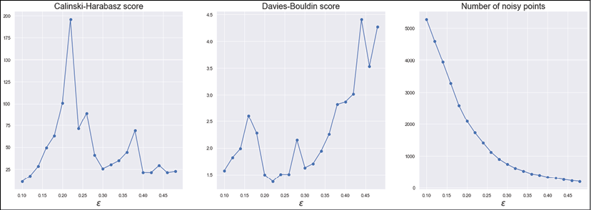
Calinski-Harabasz score (left), Davies-Bouldin score (center), the number of noisy points (right)

Let's start with the number of noisy points. As expected, the function monotonically decreases because larger values yield less cohesive clusters. However, there are two important considerations. The first one is that we need to assume a moderate number of noisy points because of the geographical structure of the map (that is, there are always suburbs or low-density areas around the centers). The second is that the function has a clear slope reduction in the range (0.2, 0.3). This indicates that, after a threshold, the number of noisy points almost stabilizes to a limit value corresponding to the total number of points that can be incorporated into clusters only when they become extremely overlapped. This is also confirmed by the Davies-Bouldin score, which increases abruptly in the same range. On the other hand, the Calinski-Harabasz score is at a maximum when and the Davies-Bouldin score is at a minimum at the same value. Therefore, also thanks to the considerations about the noisy points, we can accept as the optimal value and perform clustering with n_min = 8 and a leaf size equal to a reasonable value of (however, you can test other values and compare the performance).

from sklearn.cluster import DBSCAN
dbscan = DBSCAN(eps=0.2, min_samples=8, leaf_size=50)
Y = dbscan.fit_predict(X)
print("No. clusters: {}".format(np.unique(dbscan.labels_).shape))
print("No. noisy points: {}".format(np.sum(Y == -1)))
print("CH = {}".format(calinski_harabasz_score(X, Y)))
print("DB = {}".format(davies_bouldin_score(X, Y)))

The output of the previous snippet is:

No. clusters: (54,)
No. noisy points: 2098
CH = 100.91669074221588
DB = 1.4949468861242001

DBSCAN has determined 53 clusters (1 label is reserved for noisy points) and 2,098 noisy points (it's important to remember that different random seeds might lead to slightly different results. In this book, we always set it equal to 1,000). This value might appear very large and, in some applications, it's actually unacceptable. However, in our case, noisy points are a valuable resource to identify all low-density regions surrounding the centers, therefore we are going to keep them.

The result of the clustering procedure is shown in the following figure, where the compact dots represent noisy points:

Result of DBSCAN on the geospatial dataset. The dots represent noisy points

It's interesting to notice that DBSCAN successfully identified four dense large areas and a series of smaller ones. Indeed, the blob in the lower-left corner is the least cohesive and, looking at the plot of X, it's possible to see that it corresponds to small areas (for example, towns) very close to each other but always separated by a number of isolated points. Moreover, there are also suburbs (for example, around the top-left cluster), which are dense enough to be considered as smaller clusters. This is also a peculiar property of geographical datasets and we are going to accept them because they are semantically valid. Of course, when submitting the results to a domain expert, it's possible to receive a request, for example, to reduce the number of noisy points. We already know that the cost to pay is to have less cohesive clusters. In fact, when , it's possible to observe a drastic reduction in the number of clusters, because more and more areas become density-connected and, consequently, aggregated into single blocks.

In these cases, you can show a comparison of the results obtained using different parameter sets (including the metric – the default one is Euclidean) and explain the dynamics of DBSCAN. For instance, it's always possible to include a post-processing step to aggregate the smallest clusters, if they don't represent valid entities. Therefore, it's generally preferable to start with a lower (tuning up the value of n_min), trying to understand which blocks should be merged, instead of working with very large clusters with poor internal cohesion. As an exercise, find optimal configurations that yield less than 10, 20, and 30 clusters and compare the results that motivate the choice according to the structure of X.

Summary

In this chapter, we presented a soft-clustering method called Fuzzy C-means, which resembles the structure of standard K-means but allows managing membership degrees (analogous to probabilities) that encode the similarity of a sample with all cluster centroids. This kind of approach allows the processing of membership vectors in a more complex pipeline, where the output of a clustering process, for example, is fed into a classifier.

One of the most important limitations of K-means and similar algorithms is the symmetric structure of the clusters. This problem can be solved with methods such as spectral clustering, which is a very powerful approach based on the dataset graph and is quite similar to non-linear dimensionality reduction methods. We analyzed an algorithm proposed by Shi and Malik, showing how it can easily separate a non-convex dataset.

We also discussed a completely geometry-agnostic algorithm, DBSCAN, which is helpful when it's necessary to discover all dense regions in a complex dataset, and the Calinski-Harabasz and Davies-Boulding scores, two new evaluation measures.

In the next chapter, Chapter 8, Clustering and Unsupervised Models for Marketing, we're going to cover some unsupervised models that are very helpful for market segmentation and recommendations (in particular, biclustering) and to better understand the behavior of customers (Apriori) and suggest products according to their buyer profile.

Further reading

• Aggarwal C. C., Hinneburg A., Keim D. A., On the Surprising Behavior of Distance Metrics in High Dimensional Space, ICDT, 2001
• Arthur D., Vassilvitskii S., The Advantages of Careful Seeding, k-means++: Proceedings of the Eighteenth Annual ACM-SIAM Symposium on Discrete Algorithms, 2006
• Pedrycz W., Gomide F., An Introduction to Fuzzy Sets, The MIT Press, 1998
• Shi J., Malik J., Normalized Cuts and Image Segmentation, IEEE Transactions on Pattern Analysis and Machine Intelligence, Vol. 22, 08, 2000
• Gelfand I. M., Glagoleva E. G., Shnol E. E., Functions and Graphs Vol. 2, The MIT Press, 1969
• Biyikoglu T., Leydold J., Stadler P. F., Laplacian Eigenvectors of Graphs, Springer, 2007
• Ester M., Kriegel H. P., Sander J., Xu X., A Density-Based Algorithm for Discovering Clusters in Large Spatial Databases with Noise, Proceedings of the 2nd International Conference on Knowledge Discovery and Data Mining, AAAI Press, pp. 226-231, 1996
• Kluger Y., Basri R., Chang J. T., Gerstein M., Spectral Biclustering of Microarray Cancer Data: Co-clustering Genes and Conditions, Genome Research, 13, 2003
• Huang, S., Wang, H., Li, D., Yang, Y., Li, T., Spectral co-clustering ensemble. Knowledge-Based Systems, 84, 46-55, 2015
• Bichot, C., Co-clustering Documents and Words by Minimizing the Normalized Cut Objective Function. Journal of Mathematical Modelling and Algorithms, 9(2), 131-147, 2010
• Agrawal R., Srikant R., Fast Algorithms for Mining Association Rules, Proceedings of the 20^th VLDB Conference, 1994
• Li, Y., The application of Apriori algorithm in the area of association rules. Proceedings of SPIE, 8878, 88784H-88784H-5, 2013
• Bonaccorso G., Hands-On Unsupervised Learning with Python, Packt Publishing, 2019