11

Bayesian Networks and Hidden Markov Models

In this chapter, we're going to introduce the basic concepts of Bayesian models, which allow us to work with several scenarios where it's necessary to consider uncertainty as a structural part of the system. The discussion will focus on static (time-invariant) and dynamic methods that can be employed, where necessary, to model time sequences.

In particular, the chapter covers the following topics:

• Bayes' theorem and its applications
• Bayesian networks
• Sampling from a Bayesian network:
  • Markov chain Monte Carlo (MCMC), Gibbs, and Metropolis-Hastings
• Modeling a Bayesian network with PyMC3 and PyStan
• Hidden Markov Models (HMMs)
• Examples with the library hmmlearn

Before discussing more advanced topics, we need to introduce the basic concept of Bayesian statistics with a focus on all those aspects that are exploited by the algorithms discussed in the chapter.

Conditional probabilities and Bayes' theorem

If we have a probability space and two events A and B, the probability of A given B is called conditional probability, and it's defined as:

As the joint probability is commutative, that is, P(A, B) = P(B, A), it's possible to derive Bayes' theorem:

This theorem allows expressing a conditional probability as a function of the opposite one and the two marginal probabilities P(A) and P(B). This result is fundamental to many machine learning problems, because, as we're going to see in this and in the next chapters, normally it's easier to work with a conditional probability (for example, p(A|B)) in order to get the opposite (that is, p(B|A)), but it's hard to work directly with the probability p(B|A). A common form of this theorem can be expressed as:

Let's suppose that we need to estimate the probability of an event A given some observations B, or using the standard notation, the posterior probability of A; the previous formula expresses this value as proportional to the term P(A), which is the marginal probability of A, called prior probability, and the conditional probability of the observations B given the event A. p(B|A) is called likelihood, and defines how event A is likely to determine B. Therefore, we can summarize the relation as:

The proportion is not a limitation, because the term P(B) is always a normalizing constant that can be omitted. Of course, the reader must remember to normalize P(A, B) so that its terms always sum up to one. This is a key concept of Bayesian statistics, where we don't directly trust the prior probability, but we reweight it using the likelihood of our observations. To achieve this goal, we need to introduce the prior probability, which represents the initial knowledge (before observing the data).

This stage is very important and can lead to very different results as a function of the prior families. If the domain knowledge is consolidated, a precise prior distribution allows us to achieve a more accurate posterior distribution. Conversely, if the prior knowledge is limited, it's generally preferable to avoid specific distributions and, instead, default to so-called low- or non-informative priors.

In general, distributions that concentrate the probability in a restricted region are very informative and their entropy is low because the uncertainty is capped by the variance. For example, if we impose a prior Gaussian distribution N(1.0, 0.01), we expect the posterior to be very peaked around the mean. In this case, the likelihood term has a limited ability to change the prior belief, unless the sample size is extremely large. Conversely, if we know that the posterior mean can be found in the range (0.5, 1.5) but we are not sure about the true value, it's preferable to employ a distribution with a larger entropy, like a uniform one. This choice is low-informative, because all the values (for a continuous distribution, we can consider arbitrary small intervals) have the same probability and the likelihood has more room to find the right posterior mean.

Conjugate priors

Another important family of prior distributions are the conjugate priors with respect to a specific likelihood. A distribution P is said to be conjugate prior to Q with respect to the likelihood L if, using the Bayes' formula, , Q and P belong to same family. For example, if with known , the normal distribution is conjugate to itself, that is, the role of the likelihood is only to shift the Gaussian without altering the variance. Conjugate priors are helpful for many reasons. First, they simplify the calculations, because, given a likelihood, it's possible to find the posterior without any integration. Moreover, in some domains, the posterior is naturally expected to belong to same family of the prior distribution. For example, if we want to know whether a coin is either fair or loaded, the likelihood is obviously Bernoulli; there are only two discrete outcomes and the optimal prior distribution is the Beta, whose probability density function (p.d.f.) is defined as:

This probability distribution can easily model any binomial scenario. In fact, if , the p.d.f. is perfectly symmetric, while it becomes peaked around the extremes when one parameter is larger than the other one. For a fair coin, we expect the likelihood to alter both constants in the same way. When , the likelihood becomes binomial (as the experiments are independent) and . Therefore, the distribution degenerates into a perfectly balanced Bernoulli with p =1/2.

On the other side, if, for example, the number of heads (in a continuous model, this outcome can be equal exactly to 1) is much larger than the number of tails, (or vice versa) and the Beta distribution starts to be very peaked in a region close to the extreme 1. If , and the distribution degenerates to a Bernoulli with p = 1 (corresponding to the heads). This scenario is shown in the following figure:

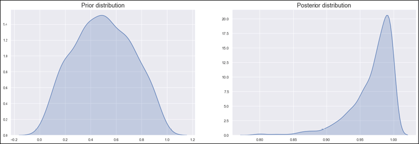
Beta prior (left) and posterior (right) distributions

It's not difficult to see that, when the likelihood is Bernoulli or binomial, the conjugate prior is Beta and, obviously, the effect of the likelihood is to shift and  in order to reproduce the actual posterior distribution.

We can now think to toss the coin 10 times (event A). We know that P(A) = 1/2 if the coin is fair. If we'd like to know what the probability is to get 10 heads, we could employ the binomial distribution obtaining P(k heads) = 1/2^k. However, let's suppose that we don't know whether the coin is fair or not, but we suspect it's loaded with a prior probability P(Coin = Loaded) = 0.7 in favor of tails. We can define a complete prior probability P(Coin) using the indicator functions:

In the previous expression, we have assumed P(Coin = Fair) = 0.5 and P(Coin = Loaded) = 0.7, the indicator I_Coin=Fair = 1 only if the coin is fair, and 0 otherwise. The same happens with I_Coin=Loaded when the coin is loaded. Our goal now is to determine the posterior probability P(Coin|B₁, B₂, …, B_n) to be able to confirm or to reject our hypothesis.

Let's imagine observing n = 10 events with B₁ = Head and B₂, …, B_n = Tail. We can express the probabilities of each outcome using the binomial distribution:

After simplifying the expression, we get:

We still need to normalize by dividing both terms by 0.083 (the sum of the two terms), so we get the final posterior probability . This result confirms and strengthens our hypothesis. The probability of a loaded coin is now about 96%, thanks to the sequence of nine tail observations after one head.

This example was presented to show how the data (observations) is plugged into the Bayesian framework. If the reader is interested in studying these concepts in more detail, in Pratt J., Raiffa H., Schlaifer R., Introduction to Statistical Decision Theory, The MIT Press, 2008, it's possible to find many interesting examples and explanations; however, before introducing Bayesian networks, it's useful to define two other essential concepts.

The first concept is called conditional independence, and it can be formalized considering two variables A and B, which are conditioned to a third one, C. We say that A and B are conditionally independent given C if:

Now, let's suppose we have an event A that is conditioned to a series of causes C₁, C₂, …, C_n. The conditional probability is, therefore, P(A|C₁, C₂, … ,C_n). Applying Bayes' theorem, we get:

If there is conditional independence, the previous expression can be simplified and rewritten as:

This property is fundamental in Naive Bayes classifiers, where we assume that the effect produced by a cause does not influence the other causes. For example, in a spam detector, we could say that the length of the mail and the presence of some particular keywords are independent events, and we only need to compute P(Length|Spam) and P(Keywords|Spam) without considering the joint probability P(Length, Keywords|Spam).

The second important element, and the last we'll analyze in this chapter, is the chain rule of probabilities. Let's suppose we have the joint probability P(X₁, X₂, … , X_n). It can be expressed as:

Repeating the procedure with the joint probability on the right side, we get:

In this way, it's possible to express a full joint probability as the product of hierarchical conditional probabilities, until the last term, which is a marginal distribution. We're going to use this concept extensively in the next section, where we'll explore Bayesian networks.

Bayesian networks

A Bayesian network is a probabilistic model represented by a direct acyclic graph G = {V, E}, where the vertices are random variables X_i, and the edges determine a conditional dependence among them. In the following diagram, there's an example of a simple Bayesian network with four variables:

Example of Bayesian network

The variable X₄ is dependent on X₃, which is dependent on X₁ and X₂. To describe the network, we need the marginal probabilities P(X₁) and P(X₂) and the conditional probabilities P(X₃ | X₁, X₂) and P(X₄ | X₃). In fact, using the chain rule, we can derive the full joint probability as:

The previous expression shows an important concept: as the graph is direct and acyclic, each variable is conditionally independent of all other variables that are not successors given its predecessors. To formalize this concept, we can define the function Predecessors(X_i), which returns the set of nodes that influence X_i directly, for example, Predecessors(X₃) = {X₁, X₂}. Using this function, it's possible to write a general expression for the full joint probability of a Bayesian network with N nodes:

The general procedure to build a Bayesian network should always start with the first causes, adding their effects one by one, until the last nodes are inserted into the graph. If this rule is not respected, the resulting graph can contain useless relations that can increase the complexity of the model. For example, if X₄ is caused indirectly by both X₁ and X₂, adding the edges and might seem like a good modeling choice; however, we know that the final influence on X₄ is determined by the value of X₃ only, whose probability is conditional on X₁ and X₂. As such, we can say with confidence that and are spurious edges, and they don't need to be added.

Sampling from a Bayesian network

Performing a direct inference on a Bayesian network can be quite a difficult operation when there's a high number of variables and edges, because the full joint probability can become extremely complex, as well as the integral needed to normalize the distribution. Since we need to compute the normalization constant to obtain the posterior probability, if this step is infeasible, we need to find other approaches to solve this problem. For this reason, several sampling methods have been proposed. In this paragraph, we're going to show how to determine the full joint probability sampling from a network using a direct approach, and two MCMC algorithms.

Let's start by considering a simple network with two connected nodes, X₁ and X₂, with the following distributions:

We can now use a direct sampling to estimate the full joint probability P(X_1, X₂) using the chain rule previously introduced.

Direct sampling

With direct sampling, our goal is to approximate the full joint probability through a sequence of samples drawn from each conditional distribution. If we assume that the graph is well structured (without unnecessary edges) and we have N variables, the algorithm is made up of the following steps:

1. Initialize the variable N_samples.
2. Initialize a vector S with shape (N, N_samples).
3. Initialize a frequency vector F_samples with shape (N, N_samples). In Python, it's better to employ a dictionary where the key is a combination (x₁, x₂, … , x_n).
4. For t = 1 to N_samples:
   1. For i = 1 to N:
      1. Sample from P(X_i | Predecessor(X_i))
      2. Store the sample in S[i, t]
   2. If F_samples contains the sampled tuple S[: , t]:
      1. 
   3. Else:
      1. (both these operations are immediate with Python dictionaries)
5. Create a vector P_sampled with shape (N, 1).
6. Set .

From a mathematical viewpoint, we are first creating a frequency vector F_samples(x₁, x₂, …, x_N; N_samples) and then approximating the full joint probability considering :

Example of direct sampling

We can now implement this algorithm in Python. Let's start by defining the sample methods using the NumPy function np.random.normal(u,s) which draws a sample from a N(u, s²) distribution:

import numpy as np
def X1_sample():
    return np.random.normal(0.1, 2.0)
def X2_sample(x1):
    return np.random.normal(x1, 0.5 + np.sqrt(np.abs(x1)))

At this point, we can implement the main cycle. Since the variables are Boolean, the total number of probabilities is 16, so we set N_samples = 10,000 (smaller values are also acceptable):

Nsamples = 10000
X = np.zeros((Nsamples, ))
Y = np.zeros((Nsamples, ))
for i, t in enumerate(range(Nsamples)):
    x1 = X1_sample()
    x2 = X2_sample(x1)
    
    X[i] = x1
    Y[i] = x2

When the sampling is complete, it's possible to visualize the density estimation of the full joint probability:

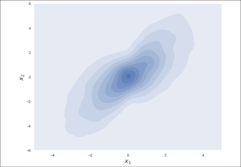
Density estimation of the full joint probability

A gentle introduction to Markov Chains

In order to discuss the MCMC algorithms, it's necessary to introduce the concept of Markov chains. In fact, while the direct sample method draws samples without any particular order, the MCMC strategies draw a sequence of samples according to a precise transition probability from a sample to the following one.

Let's consider a time-dependent random variable X(t), and let's assume a discrete time sequence X₁, X₂, … , X_t, X_t+1, … where X_t represents the value assumed at time t. In the following diagram, there's a schematic representation of this sequence:

Structure of a generic Markov chain

Suppose we have N different states , in that case, it's possible to consider the probability . X(t) is defined as a first-order Markov process if:

In other words, in a Markov process (from now on, we'll omit the specification first-order and assume that we're always working with this kind of chain, even if there are cases where it would be useful to consider a greater number of previous states), the probability that X(t) is in a certain state depends only on the state assumed in the previous time instant. Therefore, we can define a transition probability for every couple (i, j):

Considering all the couples (i, j), it's also possible to build a transition probability matrix . The marginal probability that X_t = s_i using a standard notation is defined as:

At this point, it's easy to prove (using the Chapman-Kolmogorov equation) that:

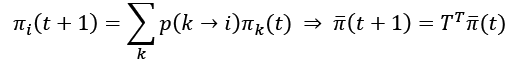
In the previous expression, in order to compute , we need to sum over all possible previous states, considering the relative transition probability. This operation can be rewritten in matrix form, using a vector containing all states and the transition probability matrix T^T (the uppercase superscript T means that the matrix is transposed). The evolution of the chain can be computed recursively:

For our purposes, it's important to consider Markov chains that are able to reach a stationary distribution :

In other words, the state does not depend on the initial condition , and it's no longer able to change. The stationary distribution is unique if the underlying Markov process is ergodic. This concept means that the process has the same properties if averaged over time (which is often impossible) or averaged vertically (freezing the time) over the states (which is simpler in the majority of cases).

The process of ergodicity for Markov chains is assured by two conditions. The first is aperiodicity for all states, which means that it is impossible to find a positive number p so that the chain returns in the same state sequence after a number of instants equal to a multiple of p. The second condition is that all states must be positive recurrent: this means that, given a random variable N_instants(i), describing the number of time instants needed to return to the state s_i, ; therefore, potentially, all the states can be revisited in a finite time.

The reason why we need the ergodicity condition, and hence the existence of a unique stationary distribution, is that we are considering the sampling processes modeled as Markov chains, where the next value is sampled according to the current state. The transition from one state to another is done in order to find better samples, as we're going to see in the Metropolis-Hastings sampler, where we can also decide to reject a sample and keep the chain in the same state. For this reason, we need to be sure that the algorithms converge to the unique stable distribution (that approximates the real full joint distribution of our Bayesian network). It's possible to prove that a chain always reaches a stationary distribution if:

The previous equation is called detailed balance and implies the reversibility of the chain. Intuitively, it means that the probability of finding the chain in the state A times the probability of a transition to the state B is equal to the probability of finding the chain in the state B times the probability of a transition to A.

For both sampling algorithms that we're going to discuss, it's possible to prove that they satisfy the previous condition, and therefore their convergence is assured.

Gibbs sampling

Let's suppose that we want to obtain the full joint probability for a Bayesian network P(X₁, X₂, …, X_N); however, the number of variables is large and there's no way to solve this problem easily in a closed form. Moreover, imagine that we would like to get a marginal distribution, such as P(X₂), but to do so we need to integrate the full joint probability, and this task is even harder. Gibbs sampling allows approximating of all marginal distributions with an iterative process. If we have N variables, the algorithm proceeds with the following steps:

• Initialize the variable N_iterations
• Initialize a vector S with shape (N, N_iterations)
• Randomly initialize (the superscript index is referred to the iteration)
• For t=1 to N_iterations:
  • Sample from and store it in S[0,t]
  • Sample from and store it in S[1,t]
  • …
  • Sample from and store it in S[N-1,t]

At the end of the iterations, vector S will contain N_iterations samples for each distribution. As we need to determine the probabilities, it's necessary to proceed like in the direct sampling algorithm, counting the number of single occurrences and normalizing dividing by N_iterations. If the variables are continuous, it's possible to consider intervals, counting how many samples are contained in each of them.

For small networks, this procedure is very similar to direct sampling, except that when working with very large networks, the sampling process could become slow; however, the algorithm can be simplified after introducing the concept of the Markov blanket of X_i, which is the set of random variables (excluding X_i) that are predecessors, successors, and successors' predecessors of X_i (in some books, they use the terms parents and children to denote these concepts). In a Bayesian network, a variable X_i is a conditional independent of all other variables given its Markov blanket. Therefore, if we define the function MB(X_i), which returns the set of variables in the blanket, the generic sampling step can be rewritten as P(X_i|MB(X_i)), and there's no more need to consider all the other variables.

To understand this concept, let's consider the network shown in the following diagram:

Bayesian network for the Gibbs sampling example

The Markov blankets of the variables are:

• MB(X₁) = {X₃}
• MB(X₂) = {X₁, X₃, X₆}
• MB(X₃) = {X₁, X₂, X₄, X₅}
• MB(X₄) = {X₃}
• MB(X₅)={X₃}
• MB(X₆)={X₂}

In general, if N is very large, the cardinality of |MB(X_i)| << N, thus simplifying the process (the vanilla Gibbs sampling needs N – 1 conditions for each variable). We can prove that the Gibbs sampling generates samples from a Markov chain that is in detailed balance:

Therefore, the procedure converges to the unique stationary distribution. This algorithm is quite simple; however, its performance is not excellent, because the random walks are not tuned up in order to explore the right regions of the state-space, where the probability to find good samples is high. Moreover, the trajectory can also return to bad states, slowing down the whole process. An alternative (also implemented by Stan for continuous random variables) is the No-U-Turn algorithm, which is not discussed in this book. The reader interested in this topic can find a full description in Hoffmann M. D., Gelman A., The No-U-Turn Sampler: Adaptively Setting Path Lengths in Hamiltonian Monte Carlo, arXiv:1111.4246, 2011.

The Metropolis-Hastings algorithm

We have seen that the full joint probability distribution of a Bayesian network P(X₁, X₂, …, X_N) can become intractable when the number of variables is large. The problem can become even harder when it's needed to marginalize it in order to obtain, for example, P(X_i), because it's necessary to integrate a very complex function. The same problem happens when applying the Bayes' theorem in simple cases.

Let's suppose we have the expression P(A|B) = KP(B|A)P(A). I've expressly inserted the normalizing constant K because if we know it, we can immediately obtain the posterior probability; however, finding it normally requires integrating P(B|A)P(A), and this operation can be impossible in closed form.

The Metropolis-Hastings algorithm can help us in solving this problem. Let's imagine that we need to sample from P(X₁, X₂, …, X_N), but we know this distribution up to a normalizing constant, so . For simplicity, from now on we collapse all variables into a single vector, so ).

Let's take another distribution , which is called candidate-generating distribution. There are no particular restrictions on this choice, only that , is easy to sample. In some situations, q can be chosen as a function very similar to the distribution , which is our target, while in other cases, it's possible to use a normal distribution with mean equal to x^(i-1). As we're going to see, this function acts as a proposal-generator, but we're not obliged to accept all the samples drawn from it; therefore, potentially any distribution with the same domain of P(X) can be employed.

When a sample is accepted, the Markov chain transitions to the next state. Otherwise, it remains in the current one. This decision process is based on the idea that the sampler must explore the most important state-space regions and discard the ones where the probability of finding good samples is low.

The algorithm proceeds with the following steps:

• Initialize the variable N_iterations
• Initialize x⁽⁰⁾ randomly
• For t=1 to N_iterations:
  • Draw a candidate sample from
  • Compute the following value:
  • If :
    • Accept the sample
  • Else if :
    • Accept the sample with probability
    • Or:
    • Reject the sample setting with probability

It's possible to prove (the proof will be omitted, but it's available in Walsh B., Markov Chain Monte Carlo and Gibbs Sampling, Lecture Notes for EEB 596z, 2002) that the transition probability of the Metropolis-Hastings algorithm satisfies the detailed balance equation (), and therefore the algorithm converges to the true posterior distribution.

Example of Metropolis-Hastings sampling

We can implement this algorithm to find the posterior distribution P(A|B) given the product of P(B|A) and P(A), without considering the normalizing constant that requires a complex integration.

Suppose that:

Therefore, the resulting g(x) (which is voluntarily relatively simple) is:

To solve this problem, we adopt the random walk Metropolis-Hastings, which consists of choosing . This choice allows simplifying the value , because the two terms and are equal (thanks to the symmetry around the vertical axis passing through x_mean) and can be canceled out, so becomes the ratio between and .

The first thing is defining the functions:

import numpy as np
def prior(x):
    return 0.1 * np.exp(-0.1 * x)
def likelihood(x):
    if x >= 0:
        return 0.5 * np.exp(-np.abs(x))
    return 0
def g(x):
    return likelihood(x) * prior(x)
def q(xp):
    return np.random.normal(xp)

Now, we can start our sampling process with 100,000 iterations and x⁽⁰⁾ = 1:

nb_iterations = 100000
x = 1.0
samples = []
for i in range(nb_iterations):
    xc = q(x)
    
    alpha = g(xc) / g(x)
    if np.isnan(alpha):
        continue
    
    if alpha >= 1:
        samples.append(xc)
        x = xc
    else:
        if np.random.uniform(0.0, 1.0) < alpha:
            samples.append(xc)
            x = xc

We can visualize the kernel density estimation and the cumulative distribution:

Sampled p.d.f. (left) and cumulative distribution (right)

Sampling using PyMC3

PyMC3 is a powerful Python Bayesian framework that relies on Theano to perform high-speed computations (it can also work using NumPy alone). It implements all the most important continuous and discrete distributions, and performs the sampling process mainly using the No-U-Turn and Metropolis-Hastings algorithms.

The example we want to model and simulate is based on this scenario: a daily flight from London to Rome has a scheduled departure time of 12:00 am, and a standard flight time of two hours. We need to organize the operations at the destination airport, but we don't want to allocate resources too long before the plane has landed. Therefore, we want to model the process using a Bayesian network, and consider some common factors that can influence the arrival time.

In particular, we know that the onboarding process can be longer than expected, as well as the refueling one, even if they're carried out in parallel. London air traffic control can impose a delay, and the same can happen when the plane is approaching Rome. We also know that the presence of rough weather can cause another delay due to rough weather forcing a change of route. We can summarize this analysis with the following plot:

Bayesian network representing the air traffic control problem

Considering our real-world experience, we decide to model the random variables using the following distributions:

• Passenger Onboarding ~ Wald()
• Refueling ~ Wald()
• Departure Traffic Delay ~ Wald()
• Arrival Traffic Delay ~ Wald()
• Departure Time = 12 + Departure Traffic Delay + max(Passenger Onboarding, Refueling)
• Rough Weather ~ Bernoulli(p=0.35)
• Flight Time ~ Exponential(=0.5 - (0.1 Rough Weather)) (The output of a Bernoulli distribution is 0 or 1, corresponding to False and True.)
• Arrival Time = Departure Time + Flight Time + Arrival Traffic Delay

The variables Departure Time and Arrival Time are functions of random variables, and the parameter of Flight Time is also a function of Rough Weather.

Even if the model's not very complex, the direct inference is rather inefficient, and therefore we want to simulate the process using PyMC3 (the package can be installed using the standard pip/conda commands as shown in http://docs.pymc.io/index.html).

The first step is to create a model instance:

import pymc3 as pm
 
 model = pm.Model()

From now on, all operations must be performed using the context manager provided by the model variable. We can now set up all the random variables of our Bayesian network:

import pymc3.distributions.continuous as pmc
import pymc3.distributions.discrete as pmd
import pymc3.math as pmm
with model:
passenger_onboarding = 
            pmc.Wald("Passenger Onboarding",
                     mu=0.5, lam=0.2)
        refueling = 
            pmc.Wald("Refueling",
                     mu=0.25, lam=0.5)
        departure_traffic_delay = 
            pmc.Wald("Departure Traffic Delay",
                     mu=0.1, lam=0.2)
        departure_time = 
            pm.Deterministic(
                "Departure Time",
                 12.0 +
                departure_traffic_delay +
                pmm.switch(
                    passenger_onboarding >= refueling,
                    passenger_onboarding,
                    refueling))
        rough_weather = 
            pmd.Bernoulli("Rough Weather",
                          p=0.35)
        flight_time = 
            pmc.Exponential("Flight Time",
                            lam=0.5 - (0.1 * rough_weather))
        arrival_traffic_delay = 
            pmc.Wald("Arrival Traffic Delay",
                     mu=0.1, lam=0.2)
        arrival_time = 
            pm.Deterministic("Arrival time",
                             departure_time +
                             flight_time +
                              arrival_traffic_delay)

We've imported two namespaces, pymc3.distributions.continuous and pymc3.distributions.discrete, because we are using both kinds of variable. Wald and exponential are continuous distributions, while Bernoulli is discrete. In the first three rows, we declare the variables passenger_onboarding, refueling, and departure_traffic_delay. The structure is always the same: we need to specify the class corresponding to the desired distribution, passing the name of the variable and all the required parameters.

The departure_time variable is declared as pm.Deterministic. In PyMC3, this means that, once all the random elements have been set, its value becomes completely determined. Indeed, if we sample from departure_traffic_delay, passenger_onboarding, and refueling, we get a determined value for departure_time. In this declaration, we've also used the utility function pmm.switch, which operates a binary choice based on its first parameter (for example, if A>B return A else return B).

The other variables are very similar, except for flight_time, which is an exponential variable with a parameter , which is a function of another variable (rough_weather). Since a Bernoulli variable outputs 1 with probability p and 0 with probability 1 – p if there's rough weather, and 0.5 otherwise.

Running the Sampling Process

Once the model has been set up, it's possible to simulate it through a sampling process. PyMC3 picks the best sampler automatically, according to the type of variables.

As the model is not very complex, we can limit the process to 500 samples using a default value of 4 chains (for more complex scenario this parameter can be increased). Moreover, as default setting, PyMC3 will skip the first 500 samples (set through the parameter draws) as the chains could have not reached the stationary distribution yet. This warm-up period is extremely important because the first samples are unreliable, and their inclusion reduces the accuracy of the posterior probability prediction. Conversely, the usage of more than one chain can help reduce the variance.

Therefore, we are going to sample a total of (500 + 500) x 4 = 4,000 data points:

nb_samples = 500
with model:
samples = pm.sample(draws=nb_samples, 
                          random_seed=1000)

The output can be analyzed using the built-in pm.traceplot() function, which generates the plots for each of the sample's variables (and each chain), as shown in the following diagram:

Distribution and samples for all random variables

The right column shown the samples generated for the random variable, while the left column shows the relative frequencies. This plot can be useful to get visual confirmation of our initial ideas; in fact, the arrival time has the majority of its mass concentrated in the interval 14:00 to 16:00 (the numbers are always decimal, so it's necessary to convert the times); however, we should integrate to get the probabilities. Instead, through the pm.summary() function, PyMC3 provides a statistical summary that can help us in making the right decisions. In the following snippet, the output containing the whole summary (which is a Pandas DataFrame) is shown:

import pandas as pd
with pd.option_context('display.max_rows', None, 
                       'display.max_columns', None):
      print(pm.summary(samples))

The output is:

                             mean        sd 
Rough Weather             0.349500  0.476812   
Passenger Onboarding      0.508697  0.792440    
Refueling                 0.248637  0.171351    
Departure Traffic Delay   0.100411  0.073563    
Departure Time           12.689327  0.775027   
Flight Time               2.231149  2.264649    
Arrival Traffic Delay     0.097987  0.066614   
Arrival time             15.018463  2.410993  
                         mc_error    hpd_2.5   hpd_97.5 
Rough Weather            0.008015   0.000000   1.000000   
Passenger Onboarding     0.021105   0.014012   1.933437   
Refueling                0.003331   0.038644   0.596968   
Departure Traffic Delay  0.001905   0.016522   0.239186   
Departure Time           0.020998  12.102561  14.099915   
Flight Time              0.053354   0.004454   6.763558   
Arrival Traffic Delay    0.001526   0.015110   0.228818   
Arrival time             0.057962  12.267486  19.823165
                               n_eff      Rhat  
Rough Weather            3518.788680  0.999277  
Passenger Onboarding     1607.397261  0.999506  
Refueling                2032.614196  0.999326  
Departure Traffic Delay  1588.997795  0.999700  
Departure Time           1396.024578  0.999855  
Flight Time              1800.353758  0.999524  
Arrival Traffic Delay    1715.607331  0.999116  
Arrival time             1787.109205  0.999169

For each variable, it contains mean, standard deviation, Monte Carlo error, 95% highest posterior density interval, and the posterior quantiles. The last two parameters (n_eff and Rhat) are extremely important to understand whether the model has reached or not a good convergence level; further details about the interpretation of these concepts will be revealed as we continue to discuss the results.

If there are more k chains, we expect that all of them become stationary, but, moreover, we need for them to all reproduce the same underlying distribution (that is, they are mixed). This goal, as proposed by Stan creators (in A. Gelman, J. B. Carlin, H. S. Stern, Bayesian Data Analysis, CRC Press, 2013), can be achieved by splitting the sequences into two parts and checking if each part is mixed with the corresponding half and with all other half parts.

The coefficient (which is called Rhat in most computer packages) has been designed to measure this result by employing a weighted average between the in-sequence and between-sequence variances of each estimated parameter (assuming N draws and the observation p):

If the distributions become stationary and the chains are properly mixed, we expect to become closer and closer to . Intuitively, it's possible to understand, that the effect of yields an overestimation of the variance, but, on the other side, when , if the model has been properly set up, the variance between sequence should approach the in-variance. Therefore, the coefficient is defined as:

In particular, when if , it means that the sequences are not properly mixed (the threshold 0.1 can be considered as a best practice), and the estimations could be inaccurate (even if theoretically , the convergence speed might be too low to assure accurate results). As it's possible to see, in our example, all , therefore we can trust the mixing result.

As the mixing is not immediate, the effective sample size (often denoted as n_eff) corresponds to the number of reliable draws (that is, obtained after the mixing). This value is less informative than , but it helps to understand whether the number of iterations is enough or it's preferable to increase it. For example, if we expect at least 1,000 draws, the result obtained in the example is satisfactory.

Conversely, if the complexity of the posterior distribution is high and we prefer at least 2,000 drawn, the simulation must be extended because the mixing time doesn't allow us to achieve this value for all parameters.

Sampling using PyStan

Let's now consider a slightly simpler example using another popular framework (Stan). Imagine that you want to model the arrival time of an airplane as a linear combination of three factors:

• Departure delay
• Travel time
• Arrival delay

Given a set of existing observations, we can assume:

However, we cannot treat the independent variables as deterministic because they are influenced by many factors which are out of our control. For example, the departure delay depends on the origin airport. The travel time is influenced by the traffic and weather conditions (moreover, there can be speed limitations imposed by the company to reduce fuel consumption). Finally, the arrival delay depends on incoming traffic. For simplicity, we're avoiding interdependencies (but I invite the reader to include them as an exercise). Given the nature of each random variable, we've decided to model them as:

As the goal of the airline is to minimize the departure delay, we've chosen an exponential distribution, whose p.d.f. is:

This distribution has a peak for x = 0 and then decreases exponentially. As longer departure delays become less and less likely, this distribution is quite reasonable. The travel time is generally the same, with limited variations around the mean; therefore, a normal distribution is the best choice.

For the arrival delay, we've made the same assumptions as we did with the departure, therefore employing another exponential with a lower (since the airplane has only a limited possibility of flying around for a long time).

Stan is based on a meta-language that is transformed into highly optimized C++ code; therefore, the first step is defining the whole model:

code = """
data {
    int<lower=0> num;
    vector[num] departure_delay;
    vector[num] travel_time;
    vector[num] arrival_delay;
    vector[num] arrival_time;
}
parameters {
    real beta_a;
    real beta_b;
    real mu_t;
    real sigma_t;
    real sigma_a;
}
model {
    departure_delay ~ exponential(beta_a);
    travel_time ~ normal(mu_t, sigma_t);
    arrival_delay ~ exponential(beta_b);
    arrival_time ~ normal(departure_delay + 
                          travel_time + 
                          arrival_delay, 
                          sigma_a);
}
"""

The code is split into four main blocks:

• data, which describes the parameters that are passed as input observations. The details of the meta-language can be found in the official documentation; however, they are very intuitive. In this case, we are declaring an integer variable num to define the number of observations and four vectors to store their values (as real – double/float – variables).
• parameters, that contains the list of estimated parameters. Each value in this block will be considered as a variable that must be estimated using a Monte Carlo algorithm.
• transformed parameters, which is missing in this case, but that normally contains all those parameters that are obtained through specific transformations (for example, functions).
• model, which contains the main structure of the code, describing the nature of every random variable and how they combine to yield to desired result. In our case, we have declared all p.d.f.s and the structure of the arrival time, which has a well-defined mean, but a variable standard deviation that is subject to estimation.

At this point, since this is an example, we can create some observations:

import numpy as np
nb_samples = 10
departure_delay = np.random.exponential(0.5, size=nb_samples)
travel_time = np.random.normal(2.0, 0.2, size=nb_samples)
arrival_delay = np.random.exponential(0.1, size=nb_samples)
arrival_time = np.random.normal(departure_delay + 
                                travel_time + 
                                arrival_delay, 
                                0.5, size=nb_samples)

In a real case, we should have collected these data through actual observations. Once the model is ready, we can compile it using PyStan (the package can be generally installed using the command pip install pystan, but the reader can find detailed instructions in the page https://pystan.readthedocs.io/en/latest/installation_beginner.html):

import pystan
model = pystan.StanModel(model_code=code)

In this way, PyStan will transform the code into a C++ module in order to achieve the best performance. Once the model has been compiled (the process can take some time depending on the available hardware), it's necessary to fit it using our data. To do that, we first need to create a dictionary where each key matches the variable name declared in the data section of the code:

data = {
    "num": nb_samples,
    "departure_delay": departure_delay,
    "arrival_time": arrival_time,
    "travel_time": travel_time,
    "arrival_delay": arrival_delay
}

Once the dictionary is ready, we can fit the model. In this case, we want to perform 10,000 iterations, with a warm-up of 1,000 draws using 2 chains:

fit = model.sampling(data=data, iter=10000, 
                     refresh=10000, warmup=1000, 
                     chains=2, seed=1000)

The result of the training procedure can be visualized directly:

print(fit)

The output of the previous code is (as a pretty print):

The summary provides information about each estimated parameter. The minimum effective sample size is greater than 5,000 and for all parameters (this is not surprising since we created the dataset, but I invite the reader to employ different distributions and check the results). In order to have a confirmation of the estimations, we can ask the model to sample from the posterior distribution:

ext = fit.extract()
beta_a = ext["beta_a"]
beta_b = ext["beta_b"]
mu_t = ext["mu_t"]
sigma_t = ext["sigma_t"]

The density estimations of the parameters are shown in the following figure:

Distribution of sampled estimations

The reader must pay attention to the difference between Stan and NumPy when working with exponential distributions. In fact, NumPy considers the parameter as , therefore, the diagrams are correct, with a peak corresponding to the true value. Considering the travel time, is normally distributed around the actual mean, while is asymmetric, indicating that larger variances are less likely than analogous smaller ones. However, the distribution has a long positive tail as . Using these values, it's possible to determine the averages and, consequently the average arrival time. In this model, we've included all the uncertainty in the prior distributions (plus the standard deviation of the arrival time), however, it's possible to work in the same way as a linear regression, structuring the model as:

In this case, the parameters can be assumed to be normally distributed, while the observed values are deterministic. It's not difficult to understand that the result is analogous to a classical regression with normally distributed residuals.

The advantage of this approach is that it's more explainable, because the magnitude of the coefficients (for example, their average and standard deviation) is directly correlated to the impact of each factor to the arrival time. The choice of a specific strategy depends on the context; however, given the flexibility of the frameworks and the computational power, I strongly suggest avoiding using deterministic variables whenever there are unmanaged uncertainty sources.

If the prior information is limited, it's always possible to default on non-informative priors (for example, uniform distributions), letting the model find the optimal parameters itself. On the other side, if the observation dataset is limited, it could be helpful to rely on domain experts to define the most reliable prior distributions (for example, in our case, we might have observed just a few flights, while an Air Traffic Controller can confirm that normally the arrival delay is close to 0 because the airport hasn't got a lot of incoming traffic).

The advantage of a Bayesian approach is evident when it's necessary to trade-off between prior knowledge and data evidence. In some cases, the former might be biased or limited, hence it's much better to rely exclusively on the data (assuming to collect enough data points). Conversely, when an expert can provide accurate details and the data points are limited, it's preferable to model the priors as expected and let the model adjust the parameters accordingly.

Hidden Markov Models

Hidden Markov Models are probabilistic algorithms that can be employed in all those contexts where it's impossible to measure the state of a system (we can only model it as a stochastic variable with a known transition probability), but it's possible to access some data connected to it. An example can be a complex engine that is made up of a large number of parts. We can define some internal states and learn a transition probability matrix (we're going to learn how to do that), but we can only receive measures provided by specific sensors.

Let's consider a stochastic process X(t) that can assume N different states: s₁, s₂, …, s_N with first-order Markov chain dynamics. Let's also suppose that we cannot observe the state of X(t), but we have access to another process O(t), connected to X(t), which produces observable outputs (often known as emissions). The resulting process is called a Hidden Markov Model (HMM), and a generic schema is shown in the following diagram:

Structure of a generic Hidden Markov Model

For each hidden state s_i, we need to define a transition probability , normally represented as a matrix if the variable is discrete. For the Markov assumption, we have:

Moreover, given a sequence of observations o₁, o₂, …, o_M we also assume the following assumption about the independence of the emission probability:

In other words, the probability of the observation o_i (in this case, we mean the value at time i) is conditioned only by the state of the hidden variable at time i (x_i). Conventionally, the first state x₀ and the last one x_ending are never emitted, and therefore all the sequences start with the index 1 and end with an extra timestep corresponding to the final state.

Sometimes, even if it's not extremely realistic, it's useful to include the Markov assumption and the emission probability independence in our models. The latter can be justified considering that we can sample all the peak emissions corresponding to precise states and, as the random process O(t) is implicitly dependent on X(t), it's not unreasonable to think of it like a pursuer of X(t).

The Markov assumption holds for many real-life processes if either they are naturally first-order Markov ones, or if the states contain all the history needed to justify a transition. In other words, in many cases, if the state is A, then there's a transit to B and finally to C. We assume that when in C, the system moved from a state (B) that carries a part of the information provided by A.

For example, if we are filling a tank, we can measure the level (the state of our system) at time t, t + 1, … If the water flow is modeled by a random variable because we don't have a stabilizer, we can find the probability that the water has reached a certain level at time t, P(L_t = x | L_t-1). Of course, it doesn't make sense to check the conditions over all the previous states, because if the level is, for example, 80m at time t – 1 then all the information needed to determine the probability of a new level (state) at time t is already contained in this state (80m).

At this point, we can start analyzing how to train an HMM, and how to determine the most likely hidden states given a sequence of observations. For simplicity, we call A the transition probability matrix, and B the matrix containing all P(o_i | x_t). The resulting model can be determined by the knowledge of those elements: HMM = {A, B}.

The Forward-Backward algorithm

The forward-backward algorithm is a simple but effective method to find the transition probability matrix T given a sequence of observations o₁, o₂, …, o_t. The first step is called the forward phase and consists of determining the probability of a sequence of observations P(o₁, o₂, …, o_{sequence length} | A, B). This piece of information can be directly useful if we need to know the likelihood of a sequence and it's necessary, together with the backward phase, to estimate the structure (A and B) of the underlying HMM.

Both algorithms are based on the concept of dynamic programming, which consists of splitting a complex problem into sub-problems that can be easily solved and reusing the solutions to solve more complex steps in a recursive/iterative fashion. For further information on this, please refer to R. A. Howard, Dynamic Programming and Markov Process, The MIT Press, 1960.

Forward phase

If we call p_ij the transition probability , we define a recursive procedure considering the following probability:

The variable represents the probability that the HMM is in the state i (at time t) after t observations (from 1 to ). Considering the HMM assumptions, we can state that depends on all possible . More precisely, we have:

With this process, we consider that the HMM can reach any of the states at time t – 1 (with the first t – 1 observations), and transition to the state i at time t with probability p_ij. We need also to consider the emission probability for the final state o_t conditioned to each of the possible previous states.

By definition, the initial and ending states are not emitting. It means that we can write any sequence of observations as 0, o₁, o₂, …, o_{sequence length}, 0 where the first and the final values are null. The procedure starts with computing the forward message at time 1:

The non-emitting ending state must be also considered:

The expression for the last state x_ending is interpreted here as the index of the ending state in both A and B matrices. For example, we indicate p_ij as A[i, j], meaning the transition probability at a generic time instant from the state x_t = i to the state x_t+1 = j. In the same way p_iending, is represented as A[i, ending] meaning the transition probability from the penultimate state x_{sequence length-1} = i to the ending one x_{sequence length-1} = ending.

The Forward algorithm can, therefore, be summarized in the following steps (we assume to have N states, hence we need to allocate N + 2 positions, considering the initial and the ending states):

1. Initialization of a Forward vector with shape (N + 2, Sequence length)
2. Initialization of A (transition probability matrix) with shape (N, N). Each element is P(x_i | x_j)
3. Initialization of B with shape (Sequence length, N). Each element is P(o_i | x_j)
4. For i = 1 to N:
   1. Set Forward[i, 1] = A[0, i]B[1, i]
5. For t = 2 to Sequence length – 1:
   1. For i = 1 to N:
      1. Set S = 0
   2. For j = 1 to N:
      1. Set S = S + Forward[j, t – 1]A[j, i]B[t, i]
   3. Set Forward [i, t] = S
6. Set S = 0
7. For i = 1 to N:
   1. Set S = S + Forward[i, Sequence length]A[i,x_ending]
8. Set Forward [x_ending, Sequence length] = S

Now it should be clear that the name "forward" derives from the procedure of propagating the information from the previous step to the next one, until the ending state, which is not emitted.

Backward phase

During the backward phase, we need to compute the probability of a sequence starting at time t + 1: o_t+1, o_t+2,…, o_{sequence length}, given that the state at time t is i. Just like we did before, we define the following probability:

The backward algorithm is very similar to the forward one, but in this case, we need to move in the opposite direction, assuming we know that the state at time t is i. The first state to consider is the last one x_ending, which like the initial state is not emitting; therefore, we have:

We terminate the recursion with the initial state:

The steps are as follows:

1. Initialization of a vector Backward with shape (N + 2, Sequence length).
2. Initialization of A (transition probability matrix) with shape (N, N). Each element is P(x_i | x_j).
3. Initialization of B with shape (Sequence length, N). Each element is P(o_i | x_j).
4. For i = 1 to N:
   1. Set Backward[x_ending, Sequence length] = A[i, x_ending]
5. For t = Sequence length – 1 to 1:
   1. For i = 1 to N:
      1. Set S = 0
      2. For j = 1 to N:
         1. Set S = S + Backward[j, t + 1]A[j, i]B[t + 1, i]
      3. Set Backward[i, t] = S
6. Set S = 0
7. For i = 1 to N:
   1. Set S = S + Backward[i, 1]A[0,i]B[1,i]
8. Set Backward[0, 1] = S

Now that we have defined both the forward and the backward algorithms, we can use them to estimate the structure of the underlying HMM.

HMM parameter estimation

The procedure we follow to estimate the parameters of the HMM is an application of the Expectation-Maximization algorithm, which will be discussed in the next chapter, Chapter 12, The EM Algorithm. Its goal can be summarized as defining how we want to estimate the values of A and B. If we define N(i, j) as the number of transitions from the state i to the state j, and N(i) the total number of transitions from the state i, we can approximate the transition probability with:

In the same way, if we define M(i, p) the number of times we have observed the emission o_p in the state i, we can approximate the emission probability P(o_p | x_i) with:

Let's start with the estimation of the transition probability matrix A. If we consider the probability that the HMM is in the state i at time t, and in the state j at time t + 1 given the observations, we have:

We can compute this probability using the forward and backward algorithms, given a sequence of observations o₁, o₂,… o_{sequence length}. In fact, we can use both the forward message , which is the probability that the HMM is in the state i after t observations, and the backward message , which is the probability of a sequence o_t+1, o_t+2, …, o_{sequence length}, starting at time t + 1, given that the HMM is in state j at time t + 1. Of course, we need also to include the emission probability and the transition probability p_ij, which is what we are estimating. The algorithm, in fact, starts with a random hypothesis and iterates until the values of A become stable. The estimation at time t is equal to:

In this context, we are omitting the full proof due to its complexity; however, the reader can find it in Rabiner L. R., A tutorial on hidden Markov models and selected applications in speech recognition, Proceedings of the IEEE 77.2, 1989.

To compute the emission probabilities, it's easier to start with the probability of being in the state i at time t given the sequence of observations:

In this case, the computation is immediate, because we can multiply the forward and backward messages computed at the same time t and state i (remember that considering the observations, the backward message is conditioned to x_t = i, while the forward message computes the probability of the observations joined with x_t = i. Hence, the multiplication is the unnormalized probability of being in the state i at time t). Therefore, we have:

The proof of how the normalizing constant is obtained can be found in the aforementioned paper. We can now plug these expressions to the estimation of a_ij and b_ip:

In the numerator of the second formula, we adopted the indicator function (it's 1 only if the condition is true, 0 otherwise) to limit the sum only where those elements are o_t = p. During an iteration k, p_ij is obtained through the estimated value found in the previous iteration k – 1.

The algorithm is based on the following steps:

1. Randomly initialize the matrices A and B.
2. Initialize a tolerance variable Tol (for example, Tol = 0.001)
3. While ||A_k – A_k-1|| > Tol and ||B_k – B_k-1|| > Tol (k is the iteration index):
   1. For t = 1 to Sequence length – 1:
      1. For i = 1 to N:
         1. For j = 1 to N:
            1. Compute
      2. Compute
   2. Compute the estimations of and and store them in A_k.

Alternatively, it's possible to fix the number of iterations, even if the best solution is using both a tolerance and a maximum number of iterations, to terminate the process when the first condition is met.

Example of HMM training with hmmlearn

For this example, we are going to use hmmlearn (installable through the command pip install hmmlearn), which is a package for HMM computations (see the information box at the end of this section for further details).

For simplicity, let's consider the airport example we discussed in the section about the Bayesian networks, and let's suppose we have a single hidden variable that represents the weather (of course, this is not a real hidden variable!), modeled as a multinomial distribution with two components (good and rough).

We observe the arrival time of our flight London-Rome (which partially depends on the weather conditions), and we want to train an HMM to infer future states and compute the posterior probability of hidden states corresponding to a given sequence.

The schema for our example is shown in the following diagram:

HMM for the weather-arrival delay problem

Let's start by defining our observation vector. As we have two states, its values will be 0 and 1. Let's assume that 0 means On-time and 1 means Delay:

import numpy as np
observations = np.array([[0], [1], [1], 
                         [0], [1], [1], 
                         [1], [0], [1],
                         [0], [0], [0], 
                         [1], [0], [1], 
                         [1], [0], [1],
                         [0], [0], [1], 
                         [0], [1], [0], 
                         [0], [0], [1],
                         [0], [1], [0], 
                         [1], [0], [0], 
                         [0], [0], [0]], 
                         dtype=np.int32)

We have 35 consecutive observations whose values are either 0 or 1.

To build the HMM, we are going to use the MultinomialHMM class, with n_components=2, n_iter=100, and random_state=1000 (it's important to always use the same seed to avoid differences in the results). The number of iterations is sometimes hard to determine; for this reason, hmmlearn provides a utility ConvergenceMonitor class that can be checked to be sure that the algorithm has successfully converged.

Now we can train our model using the fit() method, passing as argument the list of observations (the array must be always bidimensional with shape Sequence length x N_components):

from hmmlearn import hmm
hmm_model = hmm.MultinomialHMM(n_components=2,
                               n_iter=100,
                               random_state=1000)
hmm_model.fit(observations)
print(hmm_model.monitor_.converged)

The output of the previous snippet is:

True

The process is very fast, and the monitor (available as instance variable monitor) has confirmed the convergence. If the model is very big and needs to be retrained, it's also possible to check smaller values of n_iter). Once the model is trained, we can immediately visualize the transition probability matrix, which is available as an instance variable transmat_:

print('
Transition probability matrix:')
print(hmm_model.transmat_)

The output is:

Transition probability matrix:
[[0.0025384  0.9974616 ]
 [0.69191905 0.30808095]]

We can interpret these values as saying that the probability to transition from 0 (good weather) to 1 (rough weather) is higher (p₀₁ is close to 1) than the opposite, and it's more likely to remain in state 1 than in state 0 (p₀₀ is almost null). We could deduce that the observations have been collected during the winter! After explaining the Viterbi algorithm in the next section, we can also check, given some observations, what the most likely hidden state sequence is.

The Viterbi algorithm

The Viterbi algorithm is one of most common decoding algorithms for HMM. Its goal is to find the most likely hidden state sequence corresponding to a series of observations. The structure is very similar to the forward algorithm, but instead of computing the probability of a sequence of observations joined with the state at the last time instant, this algorithm looks for:

The variable represents that maximum probability of the given observation sequence joint with x_t = i, considering all possible hidden state paths (from time instant 1 to t – 1). We can compute recursively by evaluating all the multiplied by the corresponding transition probabilities p_ji and emission probability P(o_t | x_i). and always picking the maximum overall possible values of j:

The algorithm is based on a backtracking approach, using a back pointer whose recursive expression is the same as but with the argmax function instead of max:

Therefore, represents the partial sequence of hidden states x₁, x₂, …, x_t-1 that maximizes . During the recursion, we add the timesteps one by one, so the previous path could be invalidated by the last observation. That's why we need to backtrack the partial result and replace the sequence built at time t that doesn't maximize anymore.

The algorithm is based on the following steps (like in the other cases, the initial and ending states are not emitting):

1. Initialization of a vector V with shape (N + 2, Sequence length).
2. Initialization of a vector BP with shape (N + 2, Sequence length).
3. Initialization of A (transition probability matrix) with shape (N, N). Each element is P(x_i | x_j).
4. Initialization of B with shape (Sequence length, N). Each element is P(o_i | x_j).
5. For i = 1 to N:
   1. Set V[i, 1] = A[i, 0]B[1, i]
   2. BP[i, 1] = Null (or any other value that cannot be interpreted as a state)
6. For t = 1 to Sequence length:
   1. For i = 1 to N:
      1. Set .
      2. Set .
7. Set .
8. Set .
9. Reverse BP.

The output of the Viterbi algorithm is a tuple with the most likely sequence BP and the corresponding probabilities V.

Finding the most likely hidden state sequence using the Viterbi algorithm and hmmlearn

At this point, we can continue with the previous example, using our model to find the most likely hidden state sequence given a set of possible observations. We can use either the decode() method or the predict() method. The first one returns the log probability of the whole sequence and the sequence itself; however, they all use the Viterbi algorithm as a default decoder:

sequence = np.array([[1], [1], [1],
                     [0], [1], [1],
                     [1], [0], [1],
                     [0], [1], [0],
                     [1], [0], [1],
                     [1], [0], [1],
                     [1], [0], [1],
                     [0], [1], [0],
                     [1], [0], [1],
                     [1], [1], [0],
                     [0], [1], [1],
                     [0], [1], [1]],
                     dtype=np.int32)
lp, hs = hmm_model.decode(sequence)
print('
Most likely hidden state sequence:')
print(hs)
print('
Log-propability:')
print(lp)

The output of the previous snippet is:

Most likely hidden state sequence:
[0 1 1 0 1 1 1 0 1 0 1 0 1 0 1 1 0 1 1 0 1 0 1 0 1 0 1 1 1 1 0 1 1 0 1 1]
Log-propability:
-30.4899924688786

The sequence is coherent with the transition probability matrix; in fact, it's more likely the persistence of rough weather (1) than the opposite. Consequently, the transition from 1 to 0 is less likely than the one from 0 to 1. The choice of state is made by selecting the highest probability; however, in some cases, the differences are minimal (in our example, it can happen to have p = (0.49, 0.51), meaning that there's a high error chance), so it's useful to check the posterior probabilities for all the states in the sequence, as shown in the following figure:

Predicted state transitions

In our case, there are a couple of states that have , so even if the output state is 1 (rough weather), it's also useful to consider a moderate probability of observing good weather. In general, if a sequence is coherent with the transition probability previously learned (or manually input), those cases are not very common. Suppose that we want to evaluate a sequence where the weather is always good (0):

sequence0 = np.array([[0], [0], [0],
                      [0], [0], [0],
                      [0], [0], [0],
                      [0], [0], [0],
                      [0], [0], [0],
                      [0], [0], [0],
                      [0], [0], [0],
                      [0], [0], [0],
                      [0], [0], [0],
                      [0], [0], [0],
                      [0], [0], [0]],
                      dtype=np.int32)
pp0 = hmm_model.predict_proba(sequence0)

This case is very particular because we know that the transition from good to rough weather is very likely (close to 1); therefore, we can't expect a stable output. The probabilities of state transitions are shown in the following figure:

Predicted state transitions with a sequence of only good weather conditions

At the beginning, the model predicts alternate states with high probabilities. This is due to the knowledge previously acquired and encoded in the transition matrix. However, after a few steps, the probabilities tend to become close to , increasing the uncertainty. The reason of such behavior is straightforward. We have trained a model using observations that describe a scenario where a day with good weather is almost always followed by a rough weather one. Therefore, a sequence of 0s (good weather) is an anomaly that the model is unable to manage properly, defaulting to a maximum entropy sequence where both states are equally likely. This example is helpful to understand how HMMs work and where it's needed to retrain them using additional special sequences.

If, for example, during summer, a period of 15-20 sunny days is observed, this block should be included in the training set, considering a frequency of observations (to avoid biasing the model). If this approach is not sufficient because of the prevalence of good-rough weather transitions, more HMMs can be trained for each period of the year. In general, I always suggest trying different configurations and observations sequences, and to also assess the probabilities for the strangest situations (like a sequence of zero second). At that point, it's possible to retrain the model and recheck that the new evidence has been correctly processed.

The data scientist has a responsibility to understand whether the models are accurate enough, or if they require more data or alternative approaches. As an exercise, I invite the reader to alter the training sequence using also a block of consecutive good-weather observations and check if the predictions become less uncertain (closer to 0 or 1).

Summary

In this chapter, we introduced Bayesian networks, describing their structure and relations. We have seen how it's possible to build a network to model a probabilistic scenario where some elements can influence the probability of others. We have also described how to obtain the full joint probability using the most common sampling methods, which allow reducing the computational complexity through an approximation.

The most common sampling methods belong to the family of MCMC algorithms, which model the transition probability from a sample to another one as a first-order Markov chain. In particular, the Gibbs sampler is based on the assumption that it's easier to sample from a conditional distribution than work directly with the full joint probability. The method is very easy to implement, but it has some performance drawbacks that can be avoided by adopting more complex strategies.

The Metropolis-Hastings sampler, instead, works with a candidate-generating distribution and a criterion to accept or reject the samples. Both methods satisfy the detailed balance equation, which guarantees their convergence (the underlying Markov chain will reach the unique stationary distribution).

In the last part of the chapter, we introduced HMMs, which allow modeling time sequences based on observations corresponding to a series of hidden states. The main concept of such models, in fact, is the presence of unobservable states that condition the emission of a particular observation (which is observable). We discussed the main assumptions and how to build, train, and infer from a model. In particular, the Forward-Backward algorithm can be employed when it's necessary to learn the transition probability matrix and the emission probabilities, while the Viterbi algorithm is adopted to find the most likely hidden state sequence given a set of consecutive observations.

In Chapter 12, The EM Algorithm, we're going to briefly discuss the Expectation-Maximization algorithm, focusing on some important applications based on the Maximum Likelihood Estimation (MLE) approach.

Further reading

• Pratt J., Raiffa H., Schlaifer R., Introduction to Statistical Decision Theory, The MIT Press, 2008
• Hoffmann M. D., Gelman A., The No-U-Turn Sampler: Adaptively Setting Path Lengths in Hamiltonian Monte Carlo, arXiv:1111.4246, 2011
• A. Gelman, J. B. Carlin, H. S. Stern, Bayesian Data Analysis, CRC Press, 2013
• Walsh B., Markov Chain Monte Carlo and Gibbs Sampling, Lecture Notes for EEB 596z, 2002
• R. A. Howard, Dynamic Programming and Markov Process, The MIT Press, 1960
• Rabiner L. R., A tutorial on hidden Markov models and selected applications in speech recognition, Proceedings of the IEEE 77.2, 1989
• W. K. Hastings, Monte Carlo sampling methods using Markov chains and their applications, Biometrik, 57/1, 04/1970
• Kevin B. Korb, Ann E. Nicholson, Bayesian Artificial Intelligence, CRC Press, 2010
• Pearl J., Causality, Cambridge University Press, 2009
• L. E. Baum, T. Petrie, Statistical Inference for Probabilistic Functions of Finite State Markov Chains, The Annals of Mathematical Statistics, 37, 1966