23
Deep Belief Networks
In this chapter, we're going to present two probabilistic generative models that employ a set of latent variables to represent a specific data generation process. Restricted Boltzmann Machines (RBMs), proposed in 1986, are the building blocks of a more complex model, called a Deep Belief Network (DBN), which is capable of capturing complex relationships among features at different levels (in a way not dissimilar to a deep convolutional network). Both models can be used in unsupervised and supervised scenarios as preprocessors or, as is usual with DBN, fine-tuning the parameters using a standard backpropagation algorithm.
In particular, we will discuss:
- Markov random fields (MRF)
- RBM, including the Contrastive Divergence (CD-k) algorithm
- DBN with supervised and unsupervised examples
We can now discuss the fundamental theoretical concept behind this model family: the Markov random fields, showing their properties and how they can be applied to solve many specific problems.
Introduction to Markov random fields
Let's consider a set of random variables, ![]() (normally drawn from the same distribution family despite there being no restrictions about the distributions that demand this must be so), organized in an undirected graph, G = {V, E}, as shown in the following diagram:
(normally drawn from the same distribution family despite there being no restrictions about the distributions that demand this must be so), organized in an undirected graph, G = {V, E}, as shown in the following diagram:

Example of a probabilistic undirected graph
Before analyzing the properties of the graph, we need to remember that two random variables, a and b, are conditionally independent given the random variable, c, if:
If all generic couples of subsets of variables ![]() are conditionally independent given a separating subset Sk (so that all connections between variables belonging to Si to variables belonging to Sj pass through Sk), the graph is called a Markov random field (MRF).
are conditionally independent given a separating subset Sk (so that all connections between variables belonging to Si to variables belonging to Sj pass through Sk), the graph is called a Markov random field (MRF).
Given G = {V, E}, a subset containing vertices such that every couple is adjacent is called a clique (the set of all cliques is often denoted as cl(G)). For example, consider the graph shown earlier. The set {x0, x1} is a clique. Moreover, if x0 and x5 are connected, {x0, x1, x5} would be a clique too, as in the following figure:

Example of a probabilistic undirected graph with connection between x0 and x5
A maximal clique is a clique that cannot be expanded by adding new vertices. A particular family of MRF is made up of all those graphs whose joint probability distribution can be factorized as:

In this case, ![]() is the normalizing constant and the product is extended to the set of all maximal cliques. According to the Hammersley-Clifford theorem, if the joint probability density function is strictly positive, the MRF can be factorized and all the
is the normalizing constant and the product is extended to the set of all maximal cliques. According to the Hammersley-Clifford theorem, if the joint probability density function is strictly positive, the MRF can be factorized and all the ![]() functions are strictly positive too. Hence
functions are strictly positive too. Hence ![]() , after some straightforward manipulations based on the properties of logarithms, can be rewritten as a Gibbs (or Boltzmann) distribution:
, after some straightforward manipulations based on the properties of logarithms, can be rewritten as a Gibbs (or Boltzmann) distribution:

The term ![]() is called energy, as it derives from the first application of such a distribution in statistical physics. The term
is called energy, as it derives from the first application of such a distribution in statistical physics. The term ![]() is now the normalizing constant employing the standard notation. In our scenarios, we always consider graphs containing observed
is now the normalizing constant employing the standard notation. In our scenarios, we always consider graphs containing observed ![]() } and latent variables
} and latent variables ![]() . Therefore, it's useful to express the joint probability as:
. Therefore, it's useful to express the joint probability as:

Whenever it's necessary to marginalize to obtain ![]() , we can simply sum over the set
, we can simply sum over the set ![]() :
:

Unfortunately, ![]() is generally intractable and the marginalization can also be extremely complex (if not impossible). However, as we are going to see, it's generally possible to work the conditional distributions
is generally intractable and the marginalization can also be extremely complex (if not impossible). However, as we are going to see, it's generally possible to work the conditional distributions ![]() and
and ![]() , which are easier to manage and allow us to model networks where the hidden units represent latent states that are never considered alone or in a joint probability distribution, but rather in conditional forms. The most common application of this approach is the Restricted Boltzmann Machine, which we are going to discuss in the next section.
, which are easier to manage and allow us to model networks where the hidden units represent latent states that are never considered alone or in a joint probability distribution, but rather in conditional forms. The most common application of this approach is the Restricted Boltzmann Machine, which we are going to discuss in the next section.
Restricted Boltzmann Machines
A Restricted Boltzmann Machine (RBM), originally called a Harmonium, is a neural model proposed by Smolensky (in Smolensky P., Information processing in dynamical systems: Foundations of harmony theory, Parallel Distributed Processing, Vol 1, The MIT Press, 1986) that is made up of a layer of input (observable) neurons and a layer of hidden (latent) neurons. A generic structure is shown in the following diagram:

Structure of an RBM
As the undirected graph is bipartite (there are no connections between neurons belonging to the same layer), the underlying probabilistic structure is an MRF. In the original model (even if this is not a restriction), all the neurons are assumed to be Bernoulli-distributed (xi,hj = {0,1}), with a bias bi (for the observed units) and cj (for the latent neurons). The resulting energy function is:

An RBM is a probabilistic generative model that can learn a data-generating process, pdata, which is represented by the observed units but exploits the presence of the latent variables in order to model all the internal relationships.
If we summarized all the parameters in a single vector, ![]() , the Gibbs distribution becomes:
, the Gibbs distribution becomes:

The training goal of an RBM is to maximize the log-likelihood with respect to an input distribution. Hence, the first step is determining ![]() after the marginalization of the previous expression:
after the marginalization of the previous expression:

As we need to maximize the log-likelihood, it's useful to compute the gradient with respect to ![]() :
:

Applying the chain rule of derivatives, we get:

Using the conditional and joint probability equalities, the previous expression becomes:

Considering the full joint probability, after some tedious manipulations (omitted for simplicity), it's possible to derive the following conditional expressions, where ![]() is the sigmoid function:
is the sigmoid function:

At this point, we can compute the gradient of the log-likelihood with respect to each single parameter, wij, bi, and cj. Starting with wij, and considering that ![]() , we get:
, we get:

If we transform the last full joint probability into a conditional one, the previous expression can be rewritten as:

Now, considering that all the units are Bernoulli-distributed, and isolating only the jth hidden unit, it's possible to apply the simplification:

Therefore, the gradient becomes:

Analogously, we can derive the gradient of ![]() with respect to bi and cj:
with respect to bi and cj:

Hence, the first term of every gradient is very easy to compute, while the second one requires summing over all observed values. As this operation is impracticable, the only feasible alternative is an approximation based on sampling, using a method such as Gibbs sampling (for further information, see Chapter 11, Bayesian Networks and Hidden Markov Models).
However, as this algorithm samples from the conditionals ![]() and
and ![]() , rather than from the full joint distribution
, rather than from the full joint distribution ![]() , it requires the associated Markov chain to reach its stationary distribution,
, it requires the associated Markov chain to reach its stationary distribution, ![]() , in order to provide valid samples. Since we don't know how many sampling steps are required to reach
, in order to provide valid samples. Since we don't know how many sampling steps are required to reach ![]() , Gibbs sampling may also be an unfeasible solution due to its potentially high computational cost.
, Gibbs sampling may also be an unfeasible solution due to its potentially high computational cost.
Contrastive Divergence
In order to solve this problem, Hinton proposed (in Hinton G., A Practical Guide to Training Restricted Boltzmann Machines, Dept. Computer Science, University of Toronto, 2010) an alternative algorithm called CD-k. The idea is very simple but extremely effective: instead of waiting for the Markov chain to reach the stationary distribution, we sample a fixed number of times starting from a training sample at t = 0, ![]() and computing
and computing ![]() by sampling from
by sampling from ![]() . Then, the hidden vector is employed to sample the reconstruction,
. Then, the hidden vector is employed to sample the reconstruction, ![]() , from
, from ![]() . This procedure can be repeated any number of times, but in practice, a single sampling step is normally enough to ensure quite good accuracy. At this point, the gradient of the log-likelihood is approximated as (considering t steps):
. This procedure can be repeated any number of times, but in practice, a single sampling step is normally enough to ensure quite good accuracy. At this point, the gradient of the log-likelihood is approximated as (considering t steps):

The single gradients with respect to wij, bi, and cj can be easily obtained considering the preceding procedure. The term contrastive derives from the approximation of the gradient of ![]() computed at
computed at ![]() with a weighted difference between a term called the positive gradient and another defined as the negative gradient. This approach is analogous to the approximation of a derivative with this incremental ratio:
with a weighted difference between a term called the positive gradient and another defined as the negative gradient. This approach is analogous to the approximation of a derivative with this incremental ratio:

The complete RBM training algorithm, based on a single-step CD-k is (assuming that there are M training data points):
- Set the number Nh of hidden units.
- Set the number of training epochs Nepochs.
- Set a learning rate
 (for example,
  ).
). - For e = 1 to Nepochs:
- Set
 .
. - For i = 1 to M:
- Sample
 from
from  .
. - Sample a reconstruction
 from
from  .
. - Accumulate the updates for weights and biases:
 (as the outer product)
 =
= 
- Sample
- Update weights and biases:
- Set
The outer product between two vectors is defined as:

If vector ![]() has (n, 1) shape and
has (n, 1) shape and ![]() has (m, 1) shape, the result is a matrix with a (n, m) shape.
has (m, 1) shape, the result is a matrix with a (n, m) shape.
Deep Belief Networks
A belief or Bayesian network is a concept already explored in Chapter 11, Bayesian Networks and Hidden Markov Models. In this particular case, we are going to consider Belief networks where there are visible and latent variables, organized into homogeneous layers. The first layer always contains the input (visible) units, while all the remaining ones are latent. Hence, a DBN can be structured as a stack of RBMs, where each hidden layer is also the visible one of the subsequent RBM, as shown in the following diagram (the number of units can be different for each layer):
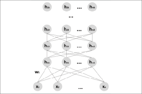
Structure of a generic DBN
The learning procedure is usually greedy and stepwise (as proposed in Hinton G. E., Osindero S., Teh Y. W., A fast learning algorithm for deep belief nets, Neural Computation, 18/7, 2006). The first RBM is trained with the dataset and optimized to reconstruct the original distribution using the CD-k algorithm. At this point, the internal (hidden) representations are employed as input for the next RBM, and so on until all the blocks are fully trained. In this way, the DBN is forced to create subsequent internal representations of the dataset that can be used for different purposes. Of course, when the model is trained, it's possible to infer from the recognition (inverse) model sampling from the hidden layers and compute the activation probability as (![]() represents a generic cause):
represents a generic cause):

As a DBN is always a generative process, in an unsupervised scenario it can perform a component analysis/dimensionality reduction, with an approach that is based on the idea of creating a chain of sub-processes that are able to rebuild an internal representation. While a single RBM focuses on a single hidden layer and hence cannot learn sub-features, a DBN greedily learns how to represent each sub-feature vector using a refined hidden distribution.
The concept behind this process isn't all that different from a cascade of convolutional layers, with the main difference being that in this case, the learning procedure is greedy. Another distinction with methods such as PCA is that we don't know exactly how the internal representation is built. As the latent variables are optimized by maximizing the log-likelihood, there are possibly many optimal points, but we cannot easily impose constraints on them.
However, DBNs show very powerful properties in different scenarios, even if their computational cost is normally considerably higher than other methods. One of the main problems (common to the majority of deep learning methods) concerns the right choice of hidden units in every layer. As they represent latent variables, their number is a crucial factor for the success of a training procedure. The right choice is not immediate because it's necessary to know the complexity of the data-generating process. However, as a rule of thumb, I suggest starting with a couple of layers containing 32/64 units and proceeding to increase the number of hidden neurons and the layers until the desired accuracy is reached (in the same way, I suggest starting with a small learning rate, such as ![]() increasing it if necessary).
increasing it if necessary).
As the first RBM is responsible for reconstructing the original dataset, it's very useful to monitor the log-likelihood (or the error) after each epoch in order to understand whether the process is learning correctly (decreasing error) or it's saturating the capacity. It's clear that an initial bad reconstruction leads to subsequently worse representations. As the learning process is greedy, in an unsupervised task there's no way to improve the performance of lower layers when the previous training steps are finished. Therefore, I always suggest tuning up the parameters so that the first reconstruction is very accurate. Of course, all the considerations about overfitting are still valid, so, it's also important to monitor the generalization ability with validation samples. However, in a component analysis, we assume we're working with a distribution that is representative of the underlying data-generating process, so the risk of finding previously seen features should be minimal.
In a supervised scenario, there are generally two options whose first step is always a greedy training of the DBN. However, the first approach performs a subsequent refinement using a standard algorithm, such as backpropagation (considering the whole architecture as a single deep network), while the second one uses the last internal representation as the input of a separate classifier.
It goes without saying that the first method has many more degrees of freedom because it works with a pre-trained network whose weights can be adjusted until the validation accuracy reaches its maximum value. In this case, the first greedy step works with the same assumption that has been empirically confirmed by observing the internal behavior of deep models (similar to convolutional networks). The first layers learn how to detect low-level features, while all the subsequent ones increase the details. Therefore, the backpropagation step presumably starts from a point that is already quite close to the optimum and can converge more quickly.
Conversely, the second approach is analogous to applying the kernel trick to a standard Support Vector Machine (SVM). In fact, the external classifier is generally a very simple one (such as a logistic regression or an SVM) and the increased accuracy is normally due to an improved linear separability obtained by projecting the original samples onto a sub-space (often higher-dimensional) where they can be easily classified. In general, this method yields worse performance than the first one because there's no way to tune up the parameters once the DBN is trained. Therefore, when the final projections are not suitable for a linear classification, it's necessary to employ more complex models and the resulting computational cost can be very high without a proportional performance gain. As deep learning is generally based on the concept of end-to-end learning, training the whole network can be useful to implicitly include the pre-processing steps in the complete structure, which becomes a black box that associates input samples with specific outcomes. On the other hand, whenever an explicit pipeline is requested, greedy training the DBN and employing a separate classifier could be a more suitable solution.
Example of an unsupervised DBN in Python
In this example, we are going to use a Python library freely available on GitHub (https://github.com/albertbup/deep-belief-network) that allows working with supervised and unsupervised DBN using NumPy (CPU-only) or TensorFlow (CPU or GPU support for versions before 2.0) with the standard scikit-learn interface. The package can be installed using the pip install git+git://github.com/albertbup/deep-belief-network.git command. However, as we are focusing our attention on TensorFlow 2.0, we are going to employ the NumPy interface.
Our goal is to create a lower-dimensional representation of a subset of the MNIST dataset (as the training process can be quite slow, we'll limit it to 400 samples), which is made up of data points ![]() . The first step is loading (using the TensorFlow/Keras helper function), shuffling, and normalizing the dataset:
. The first step is loading (using the TensorFlow/Keras helper function), shuffling, and normalizing the dataset:
import numpy as np
import tensorflow as tf
from sklearn.utils import shuffle
(X_train, Y_train), (_, _) =
        tf.keras.datasets.mnist.load_data()
X_train, Y_train = shuffle(X_train, Y_train,
                               random_state=1000)
width = X_train.shape[1]
height = X_train.shape[2]
nb_samples = 400
X = X_train[0:nb_samples].reshape(
        (nb_samples, width * height)).
            astype(np.float32) / 255.0
Y = Y_train[0:nb_samples]
At this point, we can create an instance of the UnsupervisedDBN class, setting three hidden layers with 512, 256, and 64 sigmoid units respectively (as we want to bind the values between 0 and 1), while we don't need to specify the input dimensionality as it is automatically detected from the dataset. It's easy to understand that the final goal of the model is to perform a sequential dimensionality reduction. The first RBM reduces the dimension from 784 to 512 (about 65%), and the second halves it as there 256 latent variables in the layer. Once this second representation has been optimized, the third RBM divides the dimension by 4, obtaining an output ![]() . It's important to notice that, contrary to PCA, in this case, the interdependencies between single variables (which, in this case, are pixels) are fully captured by the model.
. It's important to notice that, contrary to PCA, in this case, the interdependencies between single variables (which, in this case, are pixels) are fully captured by the model.
The learning rate ![]() (
(learning_rate_rbm), is set equal to 0.05, the batch size (batch_size) to 64, and the number of epochs for each RBM (n_epochs_rbm) to 100. The default value for the number of CD-k steps is 1, but it's possible to change it using the contrastive_divergence_iter parameter. All these values can be freely changed to improve the performance (for example, to get a smaller loss) or to speed up the training process. Our choice is based on a trade-off between accuracy and speed:
from dbn import UnsupervisedDBN
unsupervised_dbn = UnsupervisedDBN(
        hidden_layers_structure=[512, 256, 64],
        learning_rate_rbm=0.05,
        n_epochs_rbm=100,
        batch_size=64,
        activation_function='sigmoid')
X_dbn = unsupervised_dbn.fit_transform(X)
The output of this snippet is:
[START] Pre-training step:
>> Epoch 1 finished 	RBM Reconstruction error 48.407841
>> Epoch 2 finished 	RBM Reconstruction error 46.730827
…
>> Epoch 99 finished 	RBM Reconstruction error 6.486495
>> Epoch 100 finished 	RBM Reconstruction error 6.439276
[END] Pre-training step
As explained, the training process is sequential and split into pre-training and fine-tuning phases. Of course, the complexity is proportional to the number of layers and hidden units. Once this step is complete, the X_dbn array contains the values sampled from the last hidden layer. Unfortunately, this library doesn't implement an inverse transformation method, but we can use the t-SNE algorithm to project the distribution onto a bidimensional space:
from sklearn.manifold import TSNE
tsne = TSNE(n_components=2,
            perplexity=10,
            random_state=1000)
X_tsne = tsne.fit_transform(X_dbn)
The corresponding plot is shown in the following figure:

t-SNE plot of the last DBN hidden layer distribution (64-dimensional)
As you can see, even if there are still a few anomalies, the hidden low-dimensional representation is globally coherent with the original dataset. Each group containing the same digits is organized in compact clusters that preserve many geometrical properties of the original manifold where the dataset lies. For example, the group containing the digits representing a 9 is very close to the one containing the images of 7s. The groups of 3s and 8s are also very close to one another.
This result confirms that a DBN can be successfully employed as a pre-processing layer for classification purposes, but in this case, rather than reducing the dimensionality, it's often preferable to increase it in order to exploit the redundancy so we can use a simpler linear classifier (to better understand this concept, think about augmenting a dataset with polynomial features). I invite the reader to test this ability by pre-processing the whole MNIST dataset and then classifying it using logistic regression, comparing the results with a direct approach.
Example of a supervised DBN in Python
In this example, we are going to employ the Wine dataset (provided by scikit-learn), which contains data points ![]() representing the chemical properties of three different wine classes. This dataset is not extremely complex, and it can be successfully classified with simpler methods; however, the example has only a didactic purpose and can be useful for understanding how to work with this kind of data.
representing the chemical properties of three different wine classes. This dataset is not extremely complex, and it can be successfully classified with simpler methods; however, the example has only a didactic purpose and can be useful for understanding how to work with this kind of data.
The first step is to load the dataset and standardize the values by removing the mean and dividing by the standard deviation (this is very important when using, for example, ReLU units, which are equivalent to linear ones when the input is positive):
from sklearn.datasets import load_wine
from sklearn.preprocessing import StandardScaler
wine = load_wine()
ss = StandardScaler()
X = ss.fit_transform(wine['data'])
Y = wine['target']
At this point, we can create train and test sets:
from sklearn.model_selection import train_test_split
X_train, X_test, Y_train, Y_test =
        train_test_split(X, Y,
                         test_size=0.25,
                         random_state=1000)
The model is based on an instance of the SupervisedDBNClassification class, which implements the backpropagation method. The parameters are very similar to the unsupervised case, but now we can also specify the stochastic gradient descent (SGD) learning rate (learning_rate), the number of backpropagation epochs (n_iter_backprop), and an optional dropout (dropout_p). The algorithm performs an initial greedy training (whose computational cost is normally higher than the SGD phase), followed by fine-tuning. Considering the structure of the training set, we have chosen to have two hidden ReLU layers containing 16 and 8 units and to apply a dropout of 0.1 to prevent overfitting.
Considering the general behavior of these models, the two RBMs will try to find an internal representation of pdata in order to obtain the most accurate classification. In our case, the first RBM expands the dimensionality to 16 units, therefore, the hidden layer should encode some interdependency features more explicitly. The second RBM, instead, reduces the dimensionality to 8 units and it's mainly responsible to discover the manifold where the dataset lies. The choice of the structure of the network is similar to any other procedure employed in deep learning and should follow the Occam's Razor principle. Therefore, I suggest starting with very simple models and proceed by adding new layers or expanding the existing ones. Of course, the usage of dropout is highly recommended whenever the risk of overfitting is large (for example, when the dataset is very small and it's impossible to retrieve new data points):
from dbn import SupervisedDBNClassification
classifier = SupervisedDBNClassification(
        hidden_layers_structure=[16, 8],
        learning_rate_rbm=0.001,
        learning_rate=0.01,
        n_epochs_rbm=20,
        n_iter_backprop=100,
        batch_size=16,
        activation_function='relu',
        dropout_p=0.1)
classifier.fit(X_train, Y_train)
The output of the previous snippet shows the pre-training and fine-tuning losses for each epoch:
[START] Pre-training step:
>> Epoch 1 finished 	RBM Reconstruction error 12.488863
>> Epoch 2 finished 	RBM Reconstruction error 12.480352
…
>> Epoch 99 finished 	ANN training loss 1.440317
>> Epoch 100 finished 	ANN training loss 1.328146
[END] Fine tuning step
At this point, we can evaluate our model using a scikit-learn classification report:
from sklearn.metrics.classification import
    classification_report
Y_pred = classifier.predict(X_test)
print(classification_report(Y_test, Y_pred))
The output is:
              precision    recall  f1-score   support
           0       0.92      1.00      0.96        11
           1       1.00      0.90      0.95        21
           2       0.93      1.00      0.96        13
    accuracy                           0.96        45
   macro avg       0.95      0.97      0.96        45
weighted avg       0.96      0.96      0.96        45
The validation accuracy (in terms of both precision and recall) is very large (close to 0.96), but this is really a simple dataset that needs only a few minutes of training. I invite the reader to test the performance of a DBN in the classification of the MNIST/Fashion MNIST dataset, comparing the results with the one obtained using a deep convolutional network. In this case, it's important to monitor the reconstruction error of each RBM, trying to minimize it before running the backpropagation phase. At the end of this exercise, you should be able to answer this question: which is preferable, an end-to-end or a pre-processing-based approach?
Summary
In this chapter, we presented the MRF as the underlying structure of an RBM. An MRF is represented as an undirected graph whose vertices are random variables. In particular, for our purposes, we considered MRFs whose joint probability can be expressed as a product of the positive functions of each random variable. The most common distribution, based on an exponential, is called the Gibbs (or Boltzmann) distribution and it is particularly suitable for our problems because the logarithm cancels the exponential, yielding simpler expressions.
An RBM is a simple bipartite, undirected graph made up of visible and latent variables, with connections only between different groups.
The goal of this model is to learn a probability distribution, thanks to the presence of hidden units that can model the unknown relationships. Unfortunately, the log-likelihood, although very simple, cannot be easily optimized because the normalization term requires summing over all the input values. For this reason, Hinton proposed an alternative algorithm, called CD-k, which outputs an approximation of the gradient of the log-likelihood based on a fixed number (normally 1) of Gibbs sampling steps.
Stacking multiple RBMs allows us to model DBNs, where the hidden layer of each block is also the visible layer of the following one. DBNs can be trained using a greedy approach, maximizing the log-likelihood of each RBM in sequence. In an unsupervised scenario, a DBN is able to extract the features of a data-generating process in a hierarchical way, and therefore the application includes component analysis and dimensionality reduction. In a supervised scenario, a DBN can be greedily pre-trained and fine-tuned using the backpropagation algorithm (considering the whole network) or sometimes using a pre-processing step in a pipeline where the classifier is generally a very simple model (such as logistic regression).
In the next chapter, which is available online, we're going to introduce the concept of reinforcement learning, discussing the most important elements of systems that can autonomously learn to play a game or allow a robot to walk, jump, and perform tasks that are extremely difficult to model and control using classic methods.
Further reading
- Smolensky P., Information processing in dynamical systems: Foundations of harmony theory, Parallel Distributed Processing, Vol 1, The MIT Press, 1986
- Hinton G., A Practical Guide to Training Restricted Boltzmann Machines, Dept. Computer Science, University of Toronto, 2010
- Hinton G. E., Osindero S., Teh Y. W., A fast learning algorithm for deep belief nets, Neural Computation, 18/7, 2006
- Goodfellow I., Bengio Y., Courville A., Deep Learning, The MIT Press, 2016
- Bonaccorso G., Hands-On Unsupervised Learning with Python, Packt Publishing, 2019