15
Fundamentals of Ensemble Learning
In this chapter, we are going to discuss some important algorithms that exploit different estimators to improve the overall performance of an ensemble or committee. These techniques work either by introducing a medium level of randomness in every estimator belonging to a predefined set or by creating a sequence of estimators where each new model is forced to improve the performance of the previous ones. These techniques allow us to reduce both the bias and the variance (thereby increasing validation accuracy) when employing models with a limited capacity or more prone to overfit the training set.
In particular, the topics covered in the chapter are as follows:
- Introduction to ensemble learning
- A brief and propaedeutic introduction to decision trees
- Random forest and extra randomized forests
- AdaBoost (algorithms M1, SAMME, SAMME.R, and R2)
We can now start our exploration of ensemble learning algorithms by discussing the fundamental concepts of weak and strong learners and how to combine simple estimators to create much better performing committees.
Ensemble learning fundamentals
The main concept behind ensemble learning is the distinction between strong and weak learners. In particular, a strong learner is a classifier or a regressor which has enough capacity to reach the highest potential accuracy, minimizing both bias and variance (thus also achieving a satisfactory level of generalization).
On the other hand, a weak learner is a model that is generically able to achieve an accuracy slightly higher than a random guess, but whose complexity is very low (they can be trained very quickly but can never be used alone to solve complex problems).
To define a strong learner more formally, if we consider a parametrized binary classifier ![]() , we define it as a strong learner if the following is true:
, we define it as a strong learner if the following is true:

This expression can initially appear cryptic; however, it's very easy to understand. It simply expresses the concept that a strong learner is theoretically able to achieve any non-null probability of misclassification with a probability greater than or equal to 0.5 (that is, the threshold for a binary random guess).
All the models normally employed in Machine Learning tasks are normally strong learners, even though their domain can be limited (for example, a logistic regression cannot solve non-linear problems).
There is a formal definition for weak learners, too, but it's simpler to consider that the real main property of a weak learner is a limited ability to achieve a reasonable accuracy. In some very particular and small regions of the training space, a weak learner could reach a low probability of misclassification, but in the whole space its performance is only a little bit superior to a random guess. The previous one is more a theoretical definition than a practice one, because all the models currently available are normally quite a lot better than a random oracle. However, an ensemble is defined as a set of weak learners that are trained together (or in a sequence) to make up a committee. Both in classification and regression problems, the final result is obtained by averaging the predictions or employing a majority vote.
At this point, a reasonable question is—Why do we need to train many weak learners instead of a single strong one? The answer is two-pronged—in ensemble learning, we normally work with medium-strong learners (such as decision trees or linear support vector machines – SVMs) and we use them as a committee to increase the overall accuracy and reduce the variance thanks to a wider exploration of the sample space.
In fact, while a single strong learner is often able to overfit the training set, it's more difficult to keep a high accuracy over the whole sample subspace without saturating the capacity. In order to avoid overfitting, a trade-off must be found, and the result is a less accurate classifier/regressor with a simpler separation hyperplane.
The adoption of many weak learners (that are actually quite strong, because even the simplest models are more accurate than a random guess), allows us to force them to focus only on a limited subspace, so as to be able to reach a very high local accuracy with a low variance. The committee, employing an averaging technique, can easily find out which prediction is the most suitable. Alternatively, it can ask each learner to vote, assuming that a successful training process must always lead the majority to propose the most accurate classification or prediction.
The most common approaches to ensemble learning are as follows:
- Bagging (bootstrap aggregating): This approach trains n weak learners
 (very often they are decision trees) using n training sets (D1, D2, …, Dn) created by randomly sampling the original dataset D. The sampling process (called bootstrap sampling) is normally performed with replacement (which is known as proper bagging), so as to determine different data distributions. Moreover, in many real algorithms, the weak learners are also initialized and trained using a medium degree of randomness. In this way, the probability of having clones becomes very small and, at the same time, it's possible to increase the accuracy by keeping the variance under a tolerable threshold (thus avoiding overfitting). Breiman (in Breiman L., Pasting small votes for classification in large databases and on-line, Machine Learning, 36, 1999) proposed an alternative approach, called Pasting, where random selections of D are sampled without replacement. In this case, the specialization of the weak learners is more selective and focused on specific regions of the sample space without overlaps. Moreover, Ho (in Ho T., The random subspace method for constructing decision forests, Pattern Analysis and Machine Intelligence, 20, 1998), before Breiman, analyzed the possibility to create subsets by working exclusively on the features. Contrary to Pasting, this method forces the weak learners to specialize on subspaces (with sample overlaps). Such an approach resembles Cotraining, where different classifiers are employed to carry out a semi-supervised task by focusing on two different views of the dataset. However, in both cases, the requested capacity is limited, and weak learners can easily find a suitable separation hypersurface. The combination of such models, analogously to bagging, allows us to solve very complex problems through wise usage of randomness.
 - Boosting: This is an alternative approach that builds an incremental ensemble starting with a single weak learner
 and adding a new one
  at each iteration. The goal is to reweight the dataset, so as to force the new learner to focus on the data points that were previously misclassified. This strategy yields a very high accuracy because the new learners are trained with a positively biased dataset that allows them to adapt to the most difficult internal conditions.
 However, in this way, the control over the variance is weakened and the ensemble can more easily overfit the training set. It's possible to mitigate this problem by reducing the complexity of the weak learners or imposing a regularization constraint.
- Stacking: This method can be implemented in different ways, but the philosophy is always the same—use different algorithms (normally a few strong learners) trained on the same dataset and filter the final result using another classifier, averaging the predictions or using a majority vote. This strategy can be very powerful if the dataset has a structure that can be partially managed with different approaches. Each classifier or regressor should discover some data aspects that are peculiar; that's why the algorithms must be structurally different. For example, it can be useful to mix a decision tree with an SVM or linear and kernel models. The evaluation performed on the test set should clearly show the prevalence of a classifier only in some cases. If an algorithm is finally the only one that produces the best prediction, the ensemble becomes useless and it's better to focus on a single strong learner.
Random forests
A random forest is the bagging ensemble model based on decision trees. If the reader is not familiar with this kind of model, I suggest reading Alpaydin E., Introduction to Machine Learning, The MIT Press, 2010, where a complete explanation can be found. However, for our purposes, it's useful to provide a brief explanation of the most important concepts.
Random forest fundamentals
A decision tree is a model that resembles a standard hierarchical decision process. In the majority of cases, a special family is employed, called binary decision trees, as each decision yields only two outcomes. This kind of tree is often the simplest and most reasonable choice and the training process (which consists of building the tree itself) is very intuitive. The root contains the whole dataset:

Each level is obtained by applying a selection tuple, defined as follows:

The first index of the tuple corresponds to an input feature, while the threshold ti is a value chosen in the specific range of each feature. The application of a selection tuple leads to a split and two nodes that each contain a non-overlapping subset of the input dataset. In the following diagram, there's an example of a slip performed at the level of the root (initial split):

Example of initial split in a decision tree
The set X is split into two subsets defined as X11 and X12 whose data points have respectively the feature with i = 2 less or greater than the threshold ti = 0.8. The intuition behind classification decision trees is to continue splitting until the leaves contain points belonging to a single category yi (these nodes are defined as pure). In this way, a new point ![]() can traverse the tree with a computation complexity O(log M) and reach a final node that determines its category. In a very similar way, it's possible to build regression trees whose output is continuous (even if, for our purposes, we are going to consider only classification scenarios).
can traverse the tree with a computation complexity O(log M) and reach a final node that determines its category. In a very similar way, it's possible to build regression trees whose output is continuous (even if, for our purposes, we are going to consider only classification scenarios).
At this point, the main problem is how to perform each split. We cannot pick any feature and any threshold, because the final tree will be completely unbalanced and very deep. Our goal is to find the optimal selection tuple at each node considering the final goal, which is classification into discrete categories (the process is almost identical for regressions). The technique is very similar to a problem based on a cost function that must be minimized, but, in this case, we operate locally, applying an impurity measure proportional to the heterogeneity of a node. A high impurity indicates that samples belonging to many different categories are present, while an impurity equal to 0 indicates that a single category is present. As we need to continue splitting until a pure leaf appears, the optimal choice is based on a function that scores each selection tuple, allowing us to select the one that yields the lowest impurity (theoretically, the process should continue until all the leaves are pure, but normally a maximum depth is provided, so as to avoid excessive complexity).
If there are p classes, the category set can be defined as follows:

A very common impurity measure is called Gini impurity and it's based on the probability of a misclassification if a data point is categorized using a label randomly chosen from the node subset distribution. Intuitively, if all the points belong to the same category, any random choice leads to a correct classification (and the impurity becomes 0). On the other side, if the node contains points from many categories, the probability of a misclassification increases. Formally, the measure is defined as follows:

The subset is indicated by Xk and p(j | k) is obtained as the ratio of the data points belonging to the class j over the sample size. The selection tuple must be chosen so as to minimize the Gini impurity of the children. Another common approach is the cross-entropy impurity, defined as follows:

The main difference between this measure and the previous one is provided by some fundamental information theory concepts. In particular, the goal we want to reach is the minimization of the uncertainty, which is measured using the (cross-)entropy. If we have a discrete distribution and all the data points belong to the same category, a random choice can fully describe the distribution; therefore, the uncertainty is null. On the contrary, if, for example, we have a fair die, the probability of each outcome is 1/6 and the corresponding entropy is about 2.58 bits (if the base of the logarithm is 2). When the nodes become purer and purer, the cross-entropy impurity decreases and reaches 0 in an optimal scenario. Moreover, adopting the concept of mutual information, we can define the information gain obtained after a split has been performed:

Given a node, we want to create two children to maximize the information gain. In other words, by choosing the cross-entropy impurity we implicitly grow the tree until the information gain becomes null. Considering again the example of a fair die, we need 2.58 bits of information to decide which is the right outcome. If, instead, the die is loaded and the probability of an outcome is 1 (100%), we need no information to make a decision. In a decision tree, we'd like to resemble this situation, so that, when a new data point has completely traversed the tree, we don't need any further information to classify it. If a maximum depth is imposed, the final information gain cannot be null. This means that we need to pay an extra cost to finalize the classification. This cost is proportional to the residual uncertainty and should be minimized to increase the accuracy.
Other methods can also be employed (even if Gini and cross-entropy are the most common) and I invite the reader to check the references for further information. However, at this point, a consideration naturally arises. Decision trees are simple models (they are not weak learners!), but the procedure for building them is more complex than, for example, training a logistic regression or a linear SVM. Why are they so popular?
Why use Decision Trees?
One reason for the popularity of decision trees is already clear—they represent a structural process that can be shown using a diagram; however, this is not enough to justify their usage. Two important properties allow the employment of decision trees without any data preprocessing.
In fact, it's easy to understand that, contrary to other methods, there's no need for any scaling or whitening and it's possible to use continuous and categorical features at the same time. For example, if in a bidimensional dataset a feature has a variance equal to 1 and the other equal to 100, the majority of classifiers will achieve a low accuracy; therefore, a preprocessing step becomes necessary. In a decision tree, a selection tuple has the same effect also when the ranges are very different. It goes without saying that a split can be easily performed considering also categorical features and there's no need, for example, to use techniques such as one-hot encoding (which is necessary in most cases to avoid generalization errors). However, unfortunately, the separation hypersurface obtained with a decision tree is normally much more complex than the one obtained using other algorithms and this drives to a higher variance with a consequential loss of generalization ability.
To understand the reason, it's possible to imagine a very simple bidimensional dataset made up of two blobs located in the second and fourth quarters. The first set is characterized by (x < 0, y > 0), but the second one by (x < 0, y < 0). Let's also suppose that we have a few outliers, but our knowledge about the data generating process is not enough to qualify them as noisy points or outliers (the original distribution can have tails that are extended over the axes; for example, it may be a mixture of two Gaussians). In this scenario, the simplest separation line is a diagonal splitting the plane into two sub-planes containing regions belonging also to the first and third quarters. However, this decision can be made only considering both coordinates at the same time. Using a decision tree, we need to split initially, for example, using the first feature and again with the second one. The result is a piece-wise separation line (for example, splitting the plane into the region corresponding to the second quarter and its complement), leading to a very high classification variance. Paradoxically, a better solution can be obtained with an incomplete tree (limiting the process, for example, to a single split) and with the selection of the y-axis as the separation line (this is why it's important to impose a maximum depth), but the price you pay is an increased bias (and a consequently worse accuracy).
Another important element to consider when working with decision trees (and related models) is the maximum depth. It's possible to grow the tree until all the leaves are pure, but sometimes it's preferable to impose a maximum depth (and, consequently, a maximum number of terminal nodes). A maximum depth equal to 1 drives to binary models called decision stumps, which don't allow any interaction among the features (they can simply be represented as If … Then conditions). Higher values yield more terminal nodes and allow an increasing interaction among features (it's possible to think about a combination of many If … Then statements together with AND logical operators). The right value must be tuned considering every single problem and it's important to remember that very deep trees are more prone to overfitting than pruned ones.
In some contexts, it's preferable to achieve a slightly worse accuracy with a higher generalization ability and, in those cases, a maximum depth should be imposed. The most commonly used tool to determine the best value is always a grid search together with a cross-validation technique.
Random forests and the bias-variance trade-off
Random forests provide us with a powerful tool to solve the bias-variance trade-off problem. They were proposed by Breiman (in Breiman L., Random Forests, Machine Learning, 45, 2001) and their logic is very simple.
As already explained in the previous section, the bagging method starts with the choice of the number of weak learners, Nc. The second step is the generation of Nc datasets (called bootstrap samples) ![]() :
:

Each decision tree is trained using the corresponding dataset using a common impurity criterion; however, in a random forest, in order to reduce the variance, the selection splits are not computed considering all the features, but only via a random subset containing a reduced number of features (common choices are the rounded square root, log2 x or natural logarithm). This approach indeed weakens each learner, as the optimality is partially lost, but allows us to obtain a drastic variance reduction by limiting the over-specialization. At the same time, a bias reduction and an increased accuracy are a result of the ensemble (in particular for a large number of estimators). In fact, as the learners are trained with slightly different data distributions, the average of a prediction converges to the right value when ![]() (in practice, it's not always necessary to employ a very large number of decision trees, however, the correct minimum value must be found using a grid search with cross-validation). Once all the models, represented with a function
(in practice, it's not always necessary to employ a very large number of decision trees, however, the correct minimum value must be found using a grid search with cross-validation). Once all the models, represented with a function ![]() , have been trained, the final prediction can be obtained as an average:
, have been trained, the final prediction can be obtained as an average:

Alternatively, it's possible to employ a majority vote (but only for classifications):

These two methods are very similar, and, in most cases, they yield the same result. However, averaging is more robust and allows an improved flexibility when the points are almost on the boundaries. Moreover, it can be used for both classification and regression tasks.
Random forests limit their randomness by picking the best selection tuple from a smaller sample subset. In some cases, for example, when the number of features is not very large, this strategy drives to a minimum variance reduction and the computational cost is no longer justified by the result. It's possible to achieve better performances with a variant called extra-randomized trees (or simply extra-trees).
The procedure is almost the same; however, in this case, before performing a split, n random thresholds are computed (for each feature) and the one which leads to the least impurity is chosen. This approach further weakens the learners but, at the same time, reduces residual variance and prevents overfitting. The dynamic is not very different from many techniques, such as regularization or dropout (we're going to discuss this approach in the next chapter); in fact, the extra-randomness reduces the capacity of the model, forcing it to a more linearized solution (which is clearly sub-optimal).
The price to pay for this limitation is a consequent bias worsening, which, however, is compensated by the presence of many different learners. Even with random splits, when Nc is large enough, the probability of a wrong classification (or regression prediction) becomes smaller and smaller because both the average and the majority vote tend to compensate the outcome of trees whose structure is strongly sub-optimal in particular regions. This result is easier to obtain, in particular, when the number of training data points is large. In this case, in fact, sampling with replacement leads to slightly different distributions that could be considered (even if this is not formally correct) as partially and randomly boosted. Therefore, every weak learner will implicitly focus on the whole dataset with extra attention to a smaller subset that, however, is randomly selected (differently from actual boosting). Another important point to remember is that decision trees are extremely prone to overfitting (indeed, they tend to reach the final leaves with a single element per leaf). Such a condition is clearly undesirable and must be properly controlled by setting the maximum depth for each tree. In this way, the bias is kept a little bit above its potential minimum, but the ensemble has a smaller variance and can generalize better.
The complete random forest algorithm is as follows:
- Set the number of decision trees Nc
- For i = 1 to Nc:
- Create a dataset Di sampling with replacements from the original dataset X
- Set the number of features to consider during each split Nf (for example, sqrt(n))
- Set an impurity measure (for example, Gini impurity)
- Define an optional maximum depth for each tree
- For i = 1 to Nc:
- Random forest:
- Train the decision tree
 using the dataset Di and selecting the best split among Nf features randomly sampled
- Train the decision tree
- Extra-trees:
- Train the decision tree using the dataset Di, computing before each split n random thresholds and selecting the one that yields the least impurity
- Train the decision tree
- Random forest:
- Define an output function averaging the single outputs or employing a majority vote
Example of random forest with scikit-learn
In this example, we are going to use the famous Wine dataset (178 13-dimensional samples split into three classes) that is directly available in scikit-learn. Unfortunately, it's not so easy to find good and simple datasets for ensemble learning algorithms, as they are normally employed with large and complex sets that require too long a computational time. Anyway, the goal of the example is to show the properties of random forests with examples that can be run multiple times with different parameters. With this knowledge, the reader will be able to apply these models to real-life scenarios and to get the maximum advantage.
As the Wine dataset is not particularly complex, the first step is to assess the performances of different classifiers (simple Logistic Regression, Decision Tree with max depth set to 5 and cross-entropy impurity measure, and an RBF SVM of automatic tuning of ![]() ) using a 10-fold cross-validation. Even if Decision Trees and random forest are not sensitive to different scales, Logistic Regression and SVM are, therefore, after loading the dataset, we are going to scale it:
) using a 10-fold cross-validation. Even if Decision Trees and random forest are not sensitive to different scales, Logistic Regression and SVM are, therefore, after loading the dataset, we are going to scale it:
import numpy as np
from sklearn.datasets import load_wine
from sklearn.model_selection import cross_val_score
from sklearn.preprocessing import StandardScaler
from sklearn.linear_model import LogisticRegression
from sklearn.tree import DecisionTreeClassifier
from sklearn.svm import SVC
wine = load_wine()
X, Y = wine["data"], wine["target"]
ss = StandardScaler()
Xs = ss.fit_transform(X)
lr = LogisticRegression(max_iter=5000,
                        solver='lbfgs',
                        multi_class='auto',
                        random_state=1000)
scores_lr = cross_val_score(lr, Xs, Y, cv=10,
                            n_jobs=-1)
dt = DecisionTreeClassifier(criterion='entropy',
                            max_depth=5,
                            random_state=1000)
scores_dt = cross_val_score(dt, Xs, Y, cv=10,
                            n_jobs=-1)
svm = SVC(kernel='rbf',
          gamma='scale',
          random_state=1000)
scores_svm = cross_val_score(svm, Xs, Y, cv=10,
                             n_jobs=-1)
print("Avg. Logistic Regression CV Score: {:.3f}".
          format(np.mean(scores_lr)))
print("Avg. Decision Tree CV Score: {:.3f}".
          format(np.mean(scores_dt)))
print("Avg. SVM CV Score: {:.3f}".
          format(np.mean(scores_svm)))
The output is:
Avg. Logistic Regression CV Score: 0.978
Avg. Decision Tree CV Score: 0.933
Avg. SVM CV Score: 0.978
As expected, the performances are quite good, with a top value of average cross-validation accuracy equal to about 97.8% achieved by the Logistic Regression and RBF SVM. A very interesting element is the performance of the decision tree, which is slightly worse than the other classifiers. Other impurity measures (for example, Gini) or deeper trees don't improve this result, therefore, in this task, a decision tree is on average weaker than a Logistic Regression and, even if it's not fully correct, we can define this model as a candidate for our bagging test. The three curves with CV scores are shown in the following figure:

Cross-validation plots for the three test models
As it's possible to see, all classifiers tend easily to reach CV scores larger than 0.9 with 8 folds where the score is about 1.0 (no misclassifications). This means that the random forest has limited room for improvement and the ensemble must focus on the subsamples with unique features. For example, the second fold corresponds to the lowest CV scores for both classifiers, hence the data points contained in this set are the only representatives of a subregion of pdata that would be otherwise discarded. We expect the bagging ensemble to fill this gap by training some weak learners on that specific region so as to increase the final prediction confidence.
To test our hypothesis, we can now fit a random forest by instantiating the class RandomForestClassifier and selecting n_estimators=150 (I invite the reader to try different values). Considering the performances of the Decision Tree, also in this case, we are employing a cross-entropy impurity:
from sklearn.ensemble import RandomForestClassifier
rf = RandomForestClassifier(n_estimators=150,
                            n_jobs=-1,
                            criterion='entropy',
                            random_state=1000)
scores = cross_val_score(rf, Xs, Y, cv=10,
                         n_jobs=-1)
print("Avg. Random Forest CV score: {:.3f}".
          format(np.mean(scores)))
The output of the previous snippet is:
Avg. Random Forest CV score: 0.984
As expected, the average cross-validation accuracy is the highest, about 98.4%. Therefore, the random forest has successfully found a global configuration of decision trees, so as to specialize them in almost any region of the sample space. The parameter n_jobs=-1 or n_jobs=joblib.cpu_count() (including the joblib library) tells scikit-learn to parallelize the training process using all available CPU cores.
Even if we know that the random forest achieved a better average CV score, it should be helpful to also compare the standard deviation to gain a better insight about the distribution. However, in this case, it's easier to plot the scores directly:

Cross-validation plot for the random forest
Even without any other confirmation, we can be sure that the random forest has achieved a better result because all the CV scores are larger than 0.9 and 7 are close to 1.0. Of course, considering the Occam's razor principle, we should select the smallest number of trees that guarantees the largest average CV score. In the following diagram, we have plotted the average CV score as a function of the number of trees:

Average cross-validation score as a function of the number of trees
It's not surprising to observe some oscillations and a plateau when the number of trees becomes greater at about 60. The effect of the randomness can cause a performance loss, even increasing the number of learners. In fact, even if the training accuracy grows, the validation accuracy on different folds can be affected by an over-specialization. Another slight improvement appears when the number of trees becomes greater than 125 and remains almost constant for larger values. As the other classifiers have already achieved high accuracies, we have chosen Nc = 150, which should guarantee the best performances on this dataset. However, even when the computational cost is not a problem, I always suggest performing at least a grid search, in order not only to achieve the best accuracy but also to minimize the complexity of the model.
Feature importance
Another important element to consider when working with decision trees and random forests is feature importance (also called Gini importance when this impurity criterion is chosen), which is a measure proportional to the impurity reduction that a particular feature allows us to achieve. For a decision tree, it is defined as follows:

In the previous formula, n(j) denotes the number of samples reaching the node j (the sum must be extended to all nodes where the feature is chosen) and ![]() is the impurity reduction achieved at node j after splitting using the feature i. In a random forest, the importance must be computed by averaging over all trees:
is the impurity reduction achieved at node j after splitting using the feature i. In a random forest, the importance must be computed by averaging over all trees:

After fitting a model (decision tree or random forest), scikit-learn outputs the feature importance vector in the feature_importances_ instance variable. In the following graph, there's a plot showing the importance of each feature in descending order:

Feature importances for the Wine dataset
We don't want to analyze the chemical meaning of each element, but it's clear that, for example, the presence of flavonoids, proline, and color intensity are much more important than the presence of non-flavonoid phenols. As discussed in the context of regressions, when a dataset is normalized, the magnitude of the coefficients is proportional to the importance of the feature in terms of predictive power. For example, a simple logistic model can have the following structure:

If ![]() and a >> b, the value of x0 can be strong enough to push the predicted value above or below the threshold independently from x1. Analogously, the feature importance in a decision tree (or in an ensemble of trees) provides us with a measure of the ability of a feature to reduce the impurity and, consequently, to lead to a final prediction.
and a >> b, the value of x0 can be strong enough to push the predicted value above or below the threshold independently from x1. Analogously, the feature importance in a decision tree (or in an ensemble of trees) provides us with a measure of the ability of a feature to reduce the impurity and, consequently, to lead to a final prediction.
This concept is becoming more and more important and it's now called Explainable AI (XAI). The reason for such an interest derives from the requests of domain experts that want to know:
- The reasons (factors) that drove a prediction
- Which factors are negligible?
- What happens to the prediction if a factor changes (for example a patient quits smoking or takes a different medication)?
- What the prediction would be with another factor setting (for example, a domain expert can suppose a hypothesis and validate it using the model)
All these kinds of questions (and many others) cannot be easily answered using black-box models and this situation can increase the scepticism with regard to AI. On the other side, decision trees are not black-box models. The whole decision process can be plotted and it's easy to justify a prediction given the input features (even if there are more sophisticated techniques that can be employed with more complex models). Therefore, I strongly encourage the reader to analyze the feature importances and to show them to the domain experts. Moreover, as the model is working with features that are semantically independent (it's not the same for the pixels of an image), it's possible to reduce the dimensionality of a dataset by removing all those features whose importance doesn't have a high impact on the final accuracy. This process, called feature selection, should be performed using more complex statistical techniques, such as Chi-square, but when a classifier is able to produce an importance index, it's also possible to use a scikit-learn class called SelectFromModel. Passing an estimator (that can be fitted or not) and a threshold, it's possible to transform the dataset by filtering out all the features whose value is below the threshold. Applying it to our model and setting a minimum importance equal to 0.02, we get the following:
from sklearn.feature_selection import SelectFromModel
rf.fit(X, Y)
sfm = SelectFromModel(estimator=rf,
                      prefit=True,
                      threshold=0.02)
X_sfm = sfm.transform(X)
print('Feature selection shape: {}'.
          format(X_sfm.shape))
The new dataset now contains 10 features instead of the 13 of the original Wine dataset (for example, it's easy to verify that ash and non-flavonoid phenols have been removed).
Of course, as for any other dimensionality reduction method, it's always suggested you verify the final accuracy with a cross-validation and make decisions only if the trade-off between loss of accuracy and complexity reduction is reasonable. Moreover, given a dataset, it's important to remember that the predictive power of the features changes with the predicted value(s).
In other words, the feature importance is not an intrinsic property of the dataset (like the principal components), but rather is a function of the specific task. It can happen that a large dataset containing thousands of features can be reduced to a fraction of them for particular predictions, while it could completely discard them if the goal is changed. If there are more targets to predict and each of them is associated with specific predictor sets, it can be a good idea to create a pipeline that outputs the training/validation sets for each task. This approach has a clear advantage with respect to using the whole dataset, in fact, in terms of XAI, it's much easier to show the responsibilities of the important features while discarding all those factors that don't play a primary role. Moreover, the computational cost is still higher than the space cost, therefore it's not an issue to have multiple specialized copies of the same dataset if this improves the model performances and helps the domain experts in understanding the outcomes.
AdaBoost
In the previous section, we saw that sampling with a replacement leads to datasets where the data points are randomly reweighted. However, if the sample size M is very large, most of the points will appear only once and, moreover, all the choices will be totally random. AdaBoost is an algorithm proposed by Schapire and Freund that tries to maximize the efficiency of each weak learner by employing adaptive boosting (the name derives from this). In particular, the ensemble is grown sequentially, and the data distribution is recomputed at each step so as to increase the weight of those points that were misclassified and reduce the weight of the ones that were correctly classified. In this way, every new learner is forced to focus on those regions that were more problematic for the previous estimators. The reader can immediately understand that, contrary to random forests and other bagging methods, boosting doesn't rely on randomness to reduce the variance and improve the accuracy; the improvement is mainly based on weighting, rather than randomness. In fact, this method works in a deterministic way and each new data distribution is chosen with a precise goal. In this paragraph, we are going to consider a variant called Discrete AdaBoost (formally AdaBoost.M1), which needs a classifier whose output is thresholded (for example, -1 and 1). However, real-valued versions (whose output behaves like a probability) have been developed (a classical example is shown in Friedman J., Hastie T., Tibshirani R., Additive Logistic Regression: A Statistical View of Boosting, Annals of Statistics, 28/1998).
As the main concepts are always the same, the reader interested in the theoretical details of other variants can immediately find them in the referenced papers.
For simplicity, the training dataset of AdaBoost.M1 is defined as follows:

This choice is not a limitation because, in multi-class problems, a one-versus-the-rest strategy can be easily employed, even if algorithms like AdaBoost.SAMME guarantee a much better performance. In order to manipulate the data distribution, we need to define a weight set:

The weight set allows defining an implicit data distribution ![]() ), which initially is equivalent to the original one but that can be easily reshaped by changing the values wi. Once the family and the number of estimators, Nc, have been chosen, it's possible to start the global training process. The algorithm can be applied to any kind of learner that is able to produce thresholded estimations (while the real-valued variants can work with probabilities, for example, obtained through the Platt scaling method).
), which initially is equivalent to the original one but that can be easily reshaped by changing the values wi. Once the family and the number of estimators, Nc, have been chosen, it's possible to start the global training process. The algorithm can be applied to any kind of learner that is able to produce thresholded estimations (while the real-valued variants can work with probabilities, for example, obtained through the Platt scaling method).
The first instance ![]() is trained with the original dataset, which means with the data distribution
is trained with the original dataset, which means with the data distribution ![]() ). The next instances, instead, are trained with the reweighted distributions
). The next instances, instead, are trained with the reweighted distributions ![]() ),
), ![]() ), …
), … ![]() ). In order to compute them, after each training process, the normalized weighted error sum
). In order to compute them, after each training process, the normalized weighted error sum ![]() is computed:
is computed:

This value is bounded between 0 (no misclassifications) and 1 (all data points have been misclassified) and it's employed to compute the estimator weight ![]() :
:

To understand how this function works, it's useful to consider its plot (shown in the following diagram):
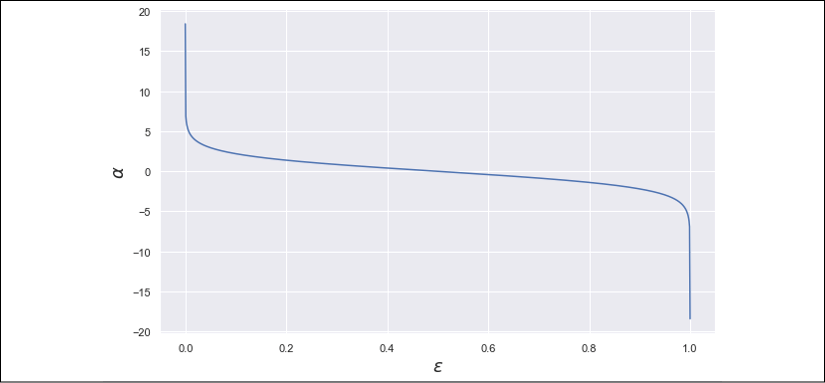
Estimator weight plot as a function of the normalized weighted error sum
This diagram unveils an implicit assumption: the worst classifier is not the one that misclassifies all points (![]() ), but a totally random binary guess (corresponding to
), but a totally random binary guess (corresponding to ![]() ). In this case,
). In this case, ![]() is null and, therefore, the outcome if the estimator is completely discarded. When
is null and, therefore, the outcome if the estimator is completely discarded. When ![]() , a boosting is applied (between about 0.05 and 0.5, the trend is almost linear), but it becomes greater than 1 only when
, a boosting is applied (between about 0.05 and 0.5, the trend is almost linear), but it becomes greater than 1 only when ![]() (larger values drive to a penalty because the weight is smaller than 1). This value is a threshold to qualify an estimator as trusted or very strong and
(larger values drive to a penalty because the weight is smaller than 1). This value is a threshold to qualify an estimator as trusted or very strong and ![]() in the particular case of a perfect estimator (no errors).
in the particular case of a perfect estimator (no errors).
In practice, an upper bound should be imposed in order to avoid overflows or divisions by zero. Instead, when ![]() , the estimator is unacceptably weak, because it's worse than a random guess and the resulting boosting would be negative. To avoid this problem, real implementations must invert the output of such estimators, transforming them de facto into learners with
, the estimator is unacceptably weak, because it's worse than a random guess and the resulting boosting would be negative. To avoid this problem, real implementations must invert the output of such estimators, transforming them de facto into learners with ![]() (this is not an issue, as the transformation is applied to all output values in the same way). It's important to consider that this algorithm shouldn't be directly applied to multi-class scenarios because, as pointed out in Zhu J., Rosset S., Zou H., Hastie T., Multi-class AdaBoost, Statistics and Its Inference, 02/2009, the threshold 0.5 corresponds to a random guess accuracy only for binary choices. When the number of classes is larger than two, a random estimator outputs a class with a probability
(this is not an issue, as the transformation is applied to all output values in the same way). It's important to consider that this algorithm shouldn't be directly applied to multi-class scenarios because, as pointed out in Zhu J., Rosset S., Zou H., Hastie T., Multi-class AdaBoost, Statistics and Its Inference, 02/2009, the threshold 0.5 corresponds to a random guess accuracy only for binary choices. When the number of classes is larger than two, a random estimator outputs a class with a probability ![]() (where Ny is the number of classes) and, therefore, AdaBoost.M1 will boost the classifiers in the wrong way, yielding poor final accuracies (the real threshold should be
(where Ny is the number of classes) and, therefore, AdaBoost.M1 will boost the classifiers in the wrong way, yielding poor final accuracies (the real threshold should be ![]() , which is larger than 0.5 when Ny > 2).
, which is larger than 0.5 when Ny > 2).
The AdaBoost.SAMME algorithm (implemented by scikit-learn) has been proposed to solve this problem and exploit the power of boosting also in multi-class scenarios.
The global decision function is defined as follows:

In this way, as the estimators are added sequentially, the importance of each of them will decrease while the accuracy of ![]() increases. However, it's also possible to observe a plateau if the complexity of X is very high. In this case, many learners will have a high weight, because the final prediction must take into account a sub-combination of learners in order to achieve an acceptable accuracy.
increases. However, it's also possible to observe a plateau if the complexity of X is very high. In this case, many learners will have a high weight, because the final prediction must take into account a sub-combination of learners in order to achieve an acceptable accuracy.
As this algorithm specializes the learners at each step, a good practice is to start with a small number of estimators (for example, 10 or 20) and increase the number until no improvement is achieved. Sometimes, a minimum number of good learners (like SVM or decision trees) is sufficient to reach the highest possible accuracy (limited to this kind of algorithm), but in some other cases, the number of estimators can be some thousands. Grid search and cross-validation are again the only good strategies to make the right choice.
After each training step it is necessary to update the weights in order to produce a boosted distribution. This is achieved using an exponential function (based on bipolar outputs {–1, 1}):

Given a data point ![]() , if it has been misclassified, its weight will be increased considering the overall estimator weight. This approach allows a further adaptive behavior because a classifier with a high
, if it has been misclassified, its weight will be increased considering the overall estimator weight. This approach allows a further adaptive behavior because a classifier with a high ![]() is already very accurate and a higher attention level is necessary to focus only on the (few) misclassified points.
is already very accurate and a higher attention level is necessary to focus only on the (few) misclassified points.
On the contrary, if ![]() is small, the estimator must improve its overall performance and the over-weighting process must be applied to a large subset (therefore, the distribution won't peak around a few points, but will penalize only the small subset that has been correctly classified, leaving the estimator free to explore the remaining space with the same probability).
is small, the estimator must improve its overall performance and the over-weighting process must be applied to a large subset (therefore, the distribution won't peak around a few points, but will penalize only the small subset that has been correctly classified, leaving the estimator free to explore the remaining space with the same probability).
Even if not present in the original proposal, it's also possible to include a learning rate ![]() that multiplies the exponent:
that multiplies the exponent:

A value ![]() has no effect, while smaller values have been proven to increase the accuracy by avoiding a premature specialization. Of course, when
has no effect, while smaller values have been proven to increase the accuracy by avoiding a premature specialization. Of course, when ![]() , the number of estimators must be increased in order to compensate the minor reweighting and this can drive to a training performance loss. As for the other hyperparameters, the right value for
, the number of estimators must be increased in order to compensate the minor reweighting and this can drive to a training performance loss. As for the other hyperparameters, the right value for ![]() must be discovered using a cross-validation technique (alternatively, if it's the only value that must be fine-tuned, it's possible to start with one and proceed by decreasing its value until the maximum accuracy has been reached).
must be discovered using a cross-validation technique (alternatively, if it's the only value that must be fine-tuned, it's possible to start with one and proceed by decreasing its value until the maximum accuracy has been reached).
The complete AdaBoost.M1 algorithm is as follows:
- Set the family and the number of estimators Nc
- Set the initial weights W(1) equal to

- Set the learning rate
 (for example,
  )
) - Set the initial distribution D(1) equal to the dataset X
- For i = 1 to Nc:
- Train the ith estimator
 with the data distribution D(i)
 - Compute the normalized weighted error sum
 :
:
- If
 , invert all estimator outputs
- If
- Compute the estimator weight

- Update the weights using the exponential formula (with or without the learning rate)
- Normalize the weights
- Train the ith estimator
- Create the global estimator applying the sign(•) function to the weighted sum

AdaBoost.SAMME
This variant, called Stagewise Additive Modeling using a Multi-class Exponential (SAMME) loss, was proposed by Zhu, Rosset, Zou, and Hastie in Zhu J., Rosset S., Zou H., Hastie T., Multi-class AdaBoost, Statistics and Its Inference, 02/2009. The goal is to adapt AdaBoost.M1 in order to work properly in multi-class scenarios.
As this is a discrete version, its structure is almost the same, with a difference in the estimator weight computation. Let's consider a label dataset Y:

Now, there are p different classes and it's necessary to consider that a random guess estimator cannot reach an accuracy equal to 0.5; therefore, the new estimator weights are computed as follows:

In this way, the threshold is pushed forward and ![]() will be zero when the following condition is true:
will be zero when the following condition is true:

The following graph shows the plot of ![]() with p = 10:
with p = 10:

Estimator weight plot as a function of the normalized weighted error sum when p = 10
Employing this correction, the boosting process can successfully cope with multi-class problems without the bias normally introduced by AdaBoost.M1 when ![]() (
(![]() when the error is less than an actual random guess, which is a function of the number of classes).
when the error is less than an actual random guess, which is a function of the number of classes).
As the performance of this algorithm is clearly superior, the majority of AdaBoost implementations aren't based on the original algorithm anymore (as already mentioned, for example, scikit-learn implements AdaBoost.SAMME and the real-valued version AdaBoost.SAMME.R). Of course, when p = 2, AdaBoost.SAMME is exactly equivalent to AdaBoost.M1.
AdaBoost.SAMME.R
AdaBoost.SAMME.R is a variant that works with classifiers that can output prediction probabilities. This is normally possible employing techniques such as Platt scaling, but it's important to check whether a specific classifier implementation is able to output the probabilities without any further action. For example, SVM implementations provided by scikit-learn don't compute the probabilities unless the parameter probability=True (because they require an extra step that could be useless in some cases).
In this case, we assume that the output of each classifier is a probability vector:

Each component is the conditional probability that the jth class is output given the input ![]() . When working with a single estimator, the winning class is obtained through the argmax x function; however, in this case, we want to re-weight each learner so as to obtain a sequentially grown ensemble. The basic idea is the same as AdaBoost.M1, but, as we now manage probability vectors, we also need an estimator weighting function that depends on the single point
. When working with a single estimator, the winning class is obtained through the argmax x function; however, in this case, we want to re-weight each learner so as to obtain a sequentially grown ensemble. The basic idea is the same as AdaBoost.M1, but, as we now manage probability vectors, we also need an estimator weighting function that depends on the single point ![]() (this function indeed wraps every single estimator that is now expressed as a probability vectorial function
(this function indeed wraps every single estimator that is now expressed as a probability vectorial function ![]() ):
):

Considering the properties of logarithms, the previous expression is equivalent to a discrete ![]() ; however, in this case, we don't rely on a weighted error sum. (The theoretical explanation is rather complex and is beyond the scope of this book. The reader can find it in the aforementioned paper, even though the method presented in Chapter 16, Advanced Boosting Algorithms, discloses a fundamental part of the logic.) To better understand the behavior of this function, let's consider a simple scenario with p = 2. The first case is a data point that the learner isn't able to classify (p = (0.5, 0.5)):
; however, in this case, we don't rely on a weighted error sum. (The theoretical explanation is rather complex and is beyond the scope of this book. The reader can find it in the aforementioned paper, even though the method presented in Chapter 16, Advanced Boosting Algorithms, discloses a fundamental part of the logic.) To better understand the behavior of this function, let's consider a simple scenario with p = 2. The first case is a data point that the learner isn't able to classify (p = (0.5, 0.5)):

In this case, the uncertainty is maximal, and the classifier cannot be trusted for this point, so the weight becomes null for all output probabilities. Now, let's apply the boosting, obtaining the probability vector p = (0.7, 0.3):

The first class will become positive and its magnitude will increase when ![]() , while the other one is the opposite value. Therefore, the functions are symmetric and allow working with a sum:
, while the other one is the opposite value. Therefore, the functions are symmetric and allow working with a sum:

This approach is very similar to a weighted majority vote because the winning class yi is computed taking into account not only the number of estimators whose output is yi but also their relative weight and the negative weight of the remaining classifiers. A class can be selected only if the strongest classifiers predicted it and the impact of the other learners is not sufficient to overturn this result.
In order to update the weights, we need to consider the impact of all probabilities. In particular, we want to reduce the uncertainty (which can degenerate to a purely random guess) and force a superior attention focused on all those points that have been misclassified. To achieve this goal, we need to define the ![]() and
and ![]() vectors, which contain, respectively, the one-hot encoding of the true class (for example, (0, 0, 1, …, 0)) and the output probabilities yielded by the estimator (as a column vector). Hence, the update rule becomes as follows:
vectors, which contain, respectively, the one-hot encoding of the true class (for example, (0, 0, 1, …, 0)) and the output probabilities yielded by the estimator (as a column vector). Hence, the update rule becomes as follows:

If, for example, the true vector is (1, 0) and the output probabilities are (0.1, 0.9), with ![]() , the weight of the point will be multiplied by about 3.16. If instead, the output probabilities are (0.9, 0.1), meaning the data point has been successfully classified, the multiplication factor will become closer to 1.
, the weight of the point will be multiplied by about 3.16. If instead, the output probabilities are (0.9, 0.1), meaning the data point has been successfully classified, the multiplication factor will become closer to 1.
In this way, the new data distribution ![]() , analogously to AdaBoost.M1, will be more peaked on the points that need more attention. All implementations include the learning rate as a hyperparameter because, as already explained, the default value equal to 1.0 cannot be the best choice for specific problems. In general, a lower learning rate allows reducing the instability when there are many outliers and improves the generalization ability thanks to a slower convergence towards the optimum. When
, analogously to AdaBoost.M1, will be more peaked on the points that need more attention. All implementations include the learning rate as a hyperparameter because, as already explained, the default value equal to 1.0 cannot be the best choice for specific problems. In general, a lower learning rate allows reducing the instability when there are many outliers and improves the generalization ability thanks to a slower convergence towards the optimum. When ![]() , every new distribution is slightly more focused on the misclassified points, allowing the estimators to search for a better parameter set without big jumps (that can lead the estimator to skip an optimal point). However, contrary to neural networks that normally work with small batches, AdaBoost can also often perform quite well with
, every new distribution is slightly more focused on the misclassified points, allowing the estimators to search for a better parameter set without big jumps (that can lead the estimator to skip an optimal point). However, contrary to neural networks that normally work with small batches, AdaBoost can also often perform quite well with ![]() because the correction is applied only after a full training step. As usual, I recommend performing a grid search to select the right values for each specific problem.
because the correction is applied only after a full training step. As usual, I recommend performing a grid search to select the right values for each specific problem.
The complete AdaBoost.SAMME.R algorithm is as follows:
- Set the family and the number of estimators Nc
- Set the initial weights W(1) equal to

- Set the learning rate
 (for example,
  )
) - Set the initial distribution D(1) equal to the dataset X
- For i = 1 to Nc:
- Train the ith estimator
 with the data distribution D(i)
 - Compute the output probabilities for each class and each training sample
- Compute the estimator weights

- Update the weights using the exponential formula (with or without the learning rate)
- Normalize the weights
- Train the ith estimator
- Create the global estimator applying the argmax x function to the sum (for i = 1 to Nc)
After discussing algorithms that work with classifiers, we can now analyze a variant that has been designed and optimized to address regression problems.
AdaBoost.R2
A slightly more complex variant has been proposed by Drucker (in Drucker H., Improving Regressors using Boosting Techniques, ICML 1997) to manage regression problems. The weak learners are commonly decision trees and the main concepts are very similar to the other variants (in particular, the re-weighting process applied to the training dataset). The real difference is the strategy adopted in order to choose the final prediction yi given the input data point ![]() . Assuming that there are Nc estimators and each of them is represented as function
. Assuming that there are Nc estimators and each of them is represented as function ![]() , we can compute the absolute residual
, we can compute the absolute residual ![]() for every input data point:
for every input data point:

Once the set Ri containing all the absolute residuals has been populated, we can compute the quantity Sr = sup Ri and compute the values of a cost function that must be proportional to the error. The common choice that is normally implemented (and suggested by the author himself) is a linear loss:

This loss is very flat and it's directly proportional to the error. In most cases, it's a good choice because it avoids premature over-specialization and allows the estimators to readapt their structure in a gentler way. The most obvious alternative is the square loss, which starts giving more importance to those points whose prediction error is larger. It is defined as follows:

The last cost function is strictly related to AdaBoost.M1 and it's exponential:

This is normally a less robust choice because, as we are also going to discuss in the next section, it penalizes small errors in favor of larger ones. Considering that these functions are also employed in the re-weighting process, an exponential loss can force the distribution to assign very high probabilities to points whose misclassification error is high, driving the estimators to become over-specialized with effect from the first iterations. In many cases (such as in neural networks), the loss functions are normally chosen according to their specific properties but, above all, according to the ease with which they can be minimized. In this particular scenario, loss functions are a fundamental part of the boosting process and they must be chosen considering the impact on the data distribution. Testing and cross-validation provide the best tool to make a reasonable decision.
Once the loss function has been evaluated for the training sample, it's possible to build the global cost function as the weighted average of all losses. Contrary to many algorithms that simply sum or average the losses, in this case, it's necessary to consider the structure of the distribution. As the boosting process reweights the points, also the corresponding loss values must be filtered to avoid a bias. At iteration t, the cost function is computed as follows:

This function is proportional to the weighted errors, which can be either linearly filtered or emphasized using a quadratic or exponential function. However, in all cases, a point whose weight is lower will yield a smaller contribution, letting the algorithm focus on the subsamples more difficult to predict. Consider that, in this case, we are working with classifications; therefore, the only measure we can exploit is the loss. Good points yield lower losses, hard ones yield proportionally higher losses. Even if it's possible to use C(t) directly, it's preferable to define a confidence measure:

This index is inversely proportional to the average confidence at iteration t. In fact, when ![]() ,
, ![]() and when
and when ![]() ,
, ![]() . The weight update is performed considering the overall confidence and the specific loss value:
. The weight update is performed considering the overall confidence and the specific loss value:

A weight will be decreased proportionally to the loss associated with the corresponding absolute residual. However, instead of using a fixed base, the global confidence index is chosen. This strategy allows a further degree of adaptability, because an estimator with a low confidence doesn't need to focus only on a small subset and, considering that ![]() is bounded between 0 and 1 (worst condition), the exponential becomes ineffective when the cost function is very high, so that the weights remain unchanged. This procedure is not very dissimilar to the one adopted in other variants, but it tries to find a trade-off between global accuracy and local misclassification problems, providing an extra degree of robustness.
is bounded between 0 and 1 (worst condition), the exponential becomes ineffective when the cost function is very high, so that the weights remain unchanged. This procedure is not very dissimilar to the one adopted in other variants, but it tries to find a trade-off between global accuracy and local misclassification problems, providing an extra degree of robustness.
The most complex part of this algorithm is the approach employed to output a global prediction. Contrary to classification algorithms, we cannot easily compute an average, because it's necessary to consider the global confidence at each iteration. Drucker proposed a method based on the weighted median of all outputs. In particular, given a point ![]() , we define the set of predictions:
, we define the set of predictions:

As weights, we consider the ![]() , so we can define a weight set:
, so we can define a weight set:

The final output is the median of Y weighted according to ![]() (normalized so that the sum is 1.0). As
(normalized so that the sum is 1.0). As ![]() when the confidence is low, the corresponding weight will tend to 0. In the same way, when the confidence is high (close to 1.0), the weight will increase proportionally and the chance to pick the output associated with it will be higher. For example, if the outputs are Y = {1, 1.2, 1.3, 2.0, 2.0, 2.5, 2.6} and the weights are
when the confidence is low, the corresponding weight will tend to 0. In the same way, when the confidence is high (close to 1.0), the weight will increase proportionally and the chance to pick the output associated with it will be higher. For example, if the outputs are Y = {1, 1.2, 1.3, 2.0, 2.0, 2.5, 2.6} and the weights are ![]() , the weighted median corresponds to the second index, therefore the global estimator will output 1.2 (which is, also intuitively, the most reasonable choice).
, the weighted median corresponds to the second index, therefore the global estimator will output 1.2 (which is, also intuitively, the most reasonable choice).
The procedure to find the median is quite simple:
- The
 must be sorted in ascending order, so that
- The set
 is sorted accordingly to the index of (each output must carry its own weight)
 - The set is normalized, dividing it by its sum
- The index corresponding to the smallest element that splits into two blocks (whose sums are less than or equal to 0.5) is selected
- The output corresponding to this index is chosen
The complete AdaBoost.R2 algorithm is as follows:
- Set the family and the number of estimators Nc
- Set the initial weights W(1) equal to
- Set the initial distribution D(1) equal to the dataset X
- Select a loss function L
- For i=1 to Nc:
- Create the global estimator using the weighted median
After a theoretical discussion about the most common AdaBoost variants, we can now focus on a practical example based on scikit-learn that can help the reader to understand how to tune up the hyperparameters and evaluate the performances.
Example of AdaBoost with scikit-learn
Let's continue using the Wine dataset in order to analyze the performance of AdaBoost with different parameters. scikit-learn, like almost all algorithms, implements both a classifier AdaBoostClassfier (based on the algorithm SAMME and SAMME.R) and a regressor AdaBoostRegressor (based on the algorithm R2). In this case, we are going to use the classifier, but I invite the reader to test the regressor using a custom dataset or one of the built-in toy datasets. In both classes, the most important parameters are n_estimators and learning_rate (default value set to 1.0).
The default underlying weak learner is always a decision tree, but it's possible to employ other models creating a base instance and passing it through the parameter base_estimator (of course, don't forget to normalize the dataset if the base classifier is sensitive to different scales). As explained in the chapter, real-valued AdaBoost algorithms require an output based on a probability vector. In scikit-learn, some classifiers/regressors (such as SVM) don't compute the probabilities unless it is explicitly required (setting the parameter probability=True); therefore, if an exception is raised, I invite you to check the documentation in order to learn how to force the algorithm to compute them.
The examples we are going to discuss have only a didactic purpose because they focus on a single parameter. In a real-world scenario, it's always better to perform a grid search (which is more expensive), so as to analyze a set of combinations. Let's start analyzing the cross-validation score as a function of the number of estimators (the vectors X and Y are the ones defined in the previous example):
import numpy as np
from sklearn.ensemble import AdaBoostClassifier
from sklearn.model_selection import cross_val_score
scores_ne = []
for ne in range(10, 201, 10):
adc = AdaBoostClassifier(n_estimators=ne,
                               learning_rate=0.8,
                               random_state=1000)
      scores_ne.append(np.mean(
          cross_val_score(adc, X, Y,
                          cv=10,
                          n_jobs=-1)))
We have considered a range starting from 10 trees and ending with 200 trees with steps of 10 trees. The learning rate is kept constant and equal to 0.8. The resulting plot is shown in the following graph:

10-fold cross-validation accuracy as a function of the number of estimators
The maximum is reached with about 125 estimators. Larger values cause slight performance worsening due to the over-specialization and a consequent variance increase, while lower values suffer a marginal lack of specialization. As explained in other chapters, the capacity of a model must be tuned according to the Occam's Razor principle, not only because the resulting model can be faster to train, but also because a capacity excess is normally saturated, overfitting the training set and reducing the scope for generalization. Cross-validation can immediately show this effect, which, instead, can remain hidden when a standard training/test set split is done (above all when the samples are not shuffled).
Let's now check the performance with different learning rates (keeping the number of trees fixed to 125):
import numpy as np
scores_eta_adc = []
for eta in np.linspace(0.01, 1.0, 100):
adc = AdaBoostClassifier(n_estimators=125,
                               learning_rate=eta,
                               random_state=1000)
       scores_eta_adc.append(
            np.mean(cross_val_score(adc, X, Y,
                    cv=10, n_jobs=-1)))
The final plot is shown in the following graph:

10-fold cross-validation accuracy as a function of the learning rate (Nc = 125)
Again, different learning rates yield different accuracies. The choice of ![]() seems to be reasonable, as higher and lower values lead to performance worsening (even if they are quite similar in a small range around 0.8). This kind of analysis should be done together with the analysis of the optimal number of trees (for example, in a grid search), however a large number of combinations might result in an extremely long search time. To avoid this problem, it's possible to perform a manual check:
seems to be reasonable, as higher and lower values lead to performance worsening (even if they are quite similar in a small range around 0.8). This kind of analysis should be done together with the analysis of the optimal number of trees (for example, in a grid search), however a large number of combinations might result in an extremely long search time. To avoid this problem, it's possible to perform a manual check:
- The number of estimators is set to a default initial value (for example, Nc = 50)
- After setting an average learning rate , the accuracy
 is assessed and compared with an expected baseline
- If
 :
:
- A lower/higher learning rate is selected, and the process is repeated
- If

- The optimal number of trees is searched after fixing
- The optimal number of trees is searched after fixing
This method is not effective as a grid search, but it can leverage the data scientist's experience to simplify the process, while guaranteeing a good compromise. Of course, all the other hyperparameters might be assessed in the same way. This can make the complexity explode, but it's possible to avoid such an overhead by starting with a single base classifier alone (for example, a Decision Tree) and tuning the specific hyperparameters. As some of them (for example, the impurity measure) have a direct impact on the ensemble, the choice can be extended to the whole model without a sensible precision loss.
As explained, the learning rate ![]() has a direct impact on the re-weighting process. Very small values require a larger number of estimators because subsequent distributions are very similar. On the other side, large values can lead to a premature over-specialization. Even if the default value is 1.0, I always suggest checking the accuracy also with smaller values. There's no golden rule for picking the right learning rate in every case, but it's important to remember that lower values allow the algorithm to smoothly adapt to fit the training set in a gentler way, while higher values reduce the robustness to outliers, because the samples that have been misclassified are immediately boosted and the probability of sampling them increases very rapidly. The result of this behavior is a constant focus on those samples that may be affected by noise, almost forgetting the structure of the remaining sample space.
has a direct impact on the re-weighting process. Very small values require a larger number of estimators because subsequent distributions are very similar. On the other side, large values can lead to a premature over-specialization. Even if the default value is 1.0, I always suggest checking the accuracy also with smaller values. There's no golden rule for picking the right learning rate in every case, but it's important to remember that lower values allow the algorithm to smoothly adapt to fit the training set in a gentler way, while higher values reduce the robustness to outliers, because the samples that have been misclassified are immediately boosted and the probability of sampling them increases very rapidly. The result of this behavior is a constant focus on those samples that may be affected by noise, almost forgetting the structure of the remaining sample space.
The last experiment we want to perform is analyzing the performance after a dimensionality reduction performed with Principal Component Analysis (PCA) and Factor Analysis (FA) (with 125 estimators and ![]() ):
):
import numpy as np
from sklearn.decomposition import PCA, FactorAnalysis
scores_pca = []
for i in range(13, 1, -1):
if i < 12:
       	pca = PCA(n_components=i,
                      random_state=1000)
            X_pca = pca.fit_transform(X)
       else:
            X_pca = X
      adc = AdaBoostClassifier(n_estimators=125,
                              learning_rate=0.8,
                              random_state=1000)
      scores_pca.append(np.mean(
cross_val_score(adc, X_pca, Y,
            n_jobs=-1, cv=10)))
scores_fa = []
for i in range(13, 1, -1):
if i < 12:
            fa = FactorAnalysis(n_components=i,
                                random_state=1000)
            X_fa = fa.fit_transform(X)
      else:
            X_fa = X
      adc = AdaBoostClassifier(n_estimators=125,
                               learning_rate=0.8,
                               random_state=1000)
      scores_fa.append(np.mean(
            cross_val_score(adc, X_fa, Y,
                            n_jobs=-1,
                            cv=10)))
The resulting plot is shown in the following graph:

10-fold cross-validation accuracy as a function of the number of components (PCA and factor analysis)
This exercise confirms some important features analyzed in Chapter 13, Component Analysis and Dimensionality Reduction. First of all, performances are not dramatically affected even by a 50% dimensionality reduction. This consideration is further confirmed by the feature importance analysis performed in the previous example. Decision trees can perform quite a good classification considering only 6/7 features because the remaining ones offer a marginal contribution to the characterization of a sample. Moreover, FA is almost always superior to PCA. With 7 components, the accuracy achieved using the FA algorithm is higher than 0.95 (very close to the value achieved with no reduction), while PCA reaches this value with 12 components. The reader should remember that PCA is a particular case of FA, with the assumption of homoscedastic noise. The diagram confirms that this condition is not acceptable with the Wine dataset. Assuming different noise variances allows remodelling the reduced dataset in a more accurate way, minimizing the cross-effect of the missing features. Even if PCA is normally the first choice, with large datasets, I suggest you always compare the performance with a Factor Analysis (FA) and choose the technique that guarantees the best result (given also that FA is more expensive in terms of computational complexity).
Summary
In this chapter, we introduced the main concepts of ensemble learning, focusing on both bagging and boosting techniques. In the first section, we explained the difference between strong and weak learners, and we presented the big picture of how it's possible to combine the estimators to achieve specific goals.
The next topic focused on the properties of decision trees and their main strengths and weaknesses. In particular, we explained that the structure of a tree causes a natural increase in the variance. The bagging technique called random forests allow mitigating this problem, improving at the same time the overall accuracy. A further variance reduction can be achieved by increasing the randomness and employing a variant called extra randomized trees. In the example, we have also seen how it's possible to evaluate the importance of each input feature and perform dimensionality reduction without involving complex statistical techniques.
In the third section, we presented the most famous boosting technique, AdaBoost, which is based on the concept of creating a sequential additive model, when each new estimator is trained using a reweighted (boosted) data distribution. In this way, every learner is added to focus on the misclassified data points without interfering with the previously added models. We analyzed the original M1 discrete variant and the most effective alternatives called SAMME and SAMME.R (real-valued), and R2 (for regressions), which are implemented in many Machine Learning packages.
In the next chapter, we are going to discuss Gradient Boosting (together with some specific highly-optimized variants) and other generalized ensemble techniques.
Further reading
- Alpaydin E., Introduction to Machine Learning, The MIT Press, 2010
- Breiman L., Bagging predictors, Machine Learning, 24, 1996
- Breiman L., Random Forests, Machine Learning, 45, 2001
- Breiman L., Pasting small votes for classification in large databases and on-line, Machine Learning, 36, 1999
- Ho T., The random subspace method for constructing decision forests, Pattern Analysis and Machine Intelligence, 20, 1998
- Friedman J., Hastie T., Tibshirani R., Additive Logistic Regression: A Statistical View of Boosting, Annals of Statistics, 28/1998
- Zhu J., Rosset S., Zou H., Hastie T., Multi-class AdaBoost, Statistics and Its Inference, 02/2009
- Drucker H., Improving Regressors using Boosting Techniques, ICML 1997
- Lundberg S. M., Lee S., A Unified Approach to Interpreting Model Predictions, Advances in Neural Information Processing Systems 30, NIPS, 2017
- Bonaccorso G., Machine Learning Algorithms Second Edition, Packt Publishing, 2018