18

Optimizing Neural Networks

In this chapter, we're going to discuss the most important optimization algorithms that have been derived from the basic Stochastic Gradient Descent (SGD) approach. This method can be quite ineffective when working with very high-dimensional functions, forcing the models to remain stuck in sub-optimal solutions. The optimizers discussed in this chapter have the goals of speeding up convergence and avoiding any sub-optimality. Moreover, we'll also discuss how to apply L₁ and L₂ regularization to a layer of a deep neural network, and how to avoid overfitting using these advanced approaches.

In particular, the topics covered in the chapter are as follows:

• Optimized SGD algorithms (Momentum, RMSProp, Adam, AdaGrad, and AdaDelta)
• Regularization techniques and dropout
• Batch normalization

After having discussed the basic concepts of neural modeling in the previous chapter, we can now start discussing how to improve the convergence speed and how to implement the most common regularization techniques.

Optimization algorithms

When we discussed the back-propagation algorithm in the previous chapter, we showed how the SGD strategy can be easily employed to train deep networks with large datasets. This method is quite robust and effective; however, the function to optimize is generally non-convex and the number of parameters is extremely large.

These conditions dramatically increase the probability of finding saddle points (instead of local minima) and can slow down the training process when the surface is almost flat (as shown in the following figure, where the point (0, 0) is a saddle point).

Example of saddle point in a hyperbolic paraboloid

Considering the previous example, as the function is f(x,y) = x² – y², the partial derivatives and the Hessian are:

Hence, the point the first partial derivatives vanishes at (0, 0), so the point is a candidate to be an extreme. However, the Hessian has the eigenvalues that are solutions of the equation , which leads to and , therefore the matrix is neither positive nor negative (semi-)definite and the point (0, 0) is a saddle point. It goes without saying that these kind of points are quite dangerous during the optimization process, because they can be located at the center of valleys where the gradient tends to vanish. In those cases, even many corrections can result in minimal movement. A common result of applying a vanilla SGD algorithm to these systems is shown in the following diagram:

Graphical representation of a real optimization process

Instead of reaching the optimal configuration, , the algorithm reaches a sub-optimal parameter configuration, , and loses the ability to perform further corrections because the gradients tend to vanish and, consequently, their contribution becomes negligible. To mitigate all these problems and their consequences, many SGD optimization algorithms have been proposed, with the purpose of speeding up convergence (also when the gradients become extremely small) and avoiding the instabilities of ill-conditioned systems.

Gradient perturbation

A common problem arises when the hypersurface is flat (plateaus) – the gradients become close to zero. A very simple way to mitigate this problem is based on adding a small homoscedastic noise component to the gradients:

The covariance matrix is normally diagonal with all elements set to , and this value is decayed during the training process to avoid perturbations when the corrections are very small. This method is conceptually reasonable, but its implicit randomness can yield undesired effects when the noise component is dominant. As it's very difficult to tune up the variances in deep models, other (more deterministic) strategies have been proposed.

Momentum and Nesterov momentum

A more robust way to improve the performance of SGD when plateaus are encountered is based on the idea of momentum (analogous to physical momentum). More formally, momentum is obtained by employing the weighted moving average of subsequent gradient estimations instead of the punctual value:

The new vector contains a component that is based on the past history (and weighted using the parameter , which is a forgetting factor) and a term referred to the current gradient estimation (multiplied by the learning rate). With this approach, abrupt changes become more difficult. When the exploration leaves a sloped region to enter a plateau, the momentum doesn't become immediately null, but for a time (proportional to ) a portion of the previous gradients will be kept, making it possible to traverse flat regions. The value assigned to the hyperparameter is normally bounded between 0 and 1. Intuitively, small values imply a short memory as the first term decays very quickly, while values close to 1.0 (for example, 0.9) allow a longer memory, less influenced by local oscillations. Like many other hyperparameters, needs to be tuned according to the specific problem, considering that a high momentum is not always the best choice. High values could slow down the convergence when very small adjustments are needed, but at the same time, values close to 0.0 are normally ineffective because the memory contribution decays too early. Using momentum, the update rule becomes as follows:

A variant is provided by Nesterov momentum, which is based on the results obtained in the field of mathematical optimization by Y. Nesterov, which has been proven to speed up the convergence of many algorithms. The idea is to determine a temporary parameter update based on the current momentum and then apply the gradient to this vector to determine the next momentum (it can be interpreted as a look-ahead gradient evaluation aimed to mitigate the risk of an incorrect correction considering the moving history of each parameter):

This algorithm showed a performance improvement in several deep models; however, its usage is still limited because, as you'll see later in this chapter, newer algorithms very soon outperformed the standard SGD with momentum, and they became the first choice in almost any real-life task.

SGD with Momentum in TensorFlow and Keras

When using TensorFlow/Keras, it's possible to customize the SGD optimizer by directly instantiating the SGD class and using it while compiling the model:

import tensorflow as tf
sgd = tf.keras.optimizers.SGD(lr=0.0001, 
                              momentum=0.8,
                              nesterov=True)
model.compile(optimizer=sgd,
              loss='categorical_crossentropy',
              metrics=['accuracy'])

The class SGD accepts the parameter lr (the learning rate with a default set equal to 0.01), momentum (the parameter ), nesterov (a Boolean indicating whether Nesterov momentum is employed), and an optional decay parameter to indicate whether the learning rate must be decayed over the updates with the following formula:

Obviously, when decay = 0, the learning rate remains constant throughout the training process. With positive values, it starts decaying with a speed inversely proportional to decay.

In the following figure, three decayed learning rates are shown:

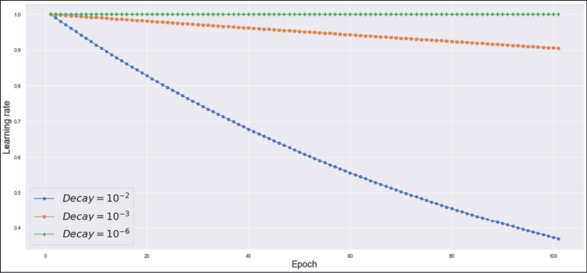
Plot of a learning rate decayed over 100 epochs with 3 different decay values

As it's possible to see, with the default value of decay = 10^-2, a hypothetical initial learning rate reaches 0.5 after about 50 epochs and it's slightly lower than 0.4 at the end of the training process. As expected, exponentially smaller decays have a dramatic impact on the learning rate. For example, decay = 10^-3 reaches 0.9 at the end of the process, while decay = 10^-6 has almost no impact. We are going to use this very value in most of our examples; in particular, when the number of epochs is not extremely large (for example, n < 200) and, with an almost constant learning rate, we keep observing a constant training/validation loss decrease throughout the process. Instead, in cases where the performance becomes worse after a number of epochs, it probably means that the algorithm has reached the basin of a minimum but keeps on jumping on the sides without reaching it. In these cases, smaller learning rates can help to improve the accuracy with a proportionally longer training process.

RMSProp

RMSProp was proposed by G. Hinton as an adaptive algorithm, partially based on the concept of momentum. Instead of considering the whole gradient vector, it tries to optimize each parameter separately to increase the corrections of slowly changing weights (which probably need more drastic modifications) and decreases the update magnitudes of quickly changing ones (which are normally the more unstable). The algorithm computes the exponentially weighted moving average of the changing speed of every parameter considering the square of the gradient (which is insensitive to the sign):

The weight update is then performed, as follows:

The parameter is a small constant (such as 10^-6) that is added to avoid numerical instabilities when the changing speed becomes null. The previous expression could be rewritten in a more compact way:

Using this notation, it is clear that the role of RMSProp is adapting the learning rate for every parameter so that it can increase it when necessary (almost frozen weights) and decrease it when the risk of oscillations is higher. In a practical implementation, the learning rate is always decayed over the epochs using an exponential or linear function.

RMSProp in TensorFlow and Keras

The following snippet shows the usage of RMSProp with TensorFlow/Keras:

import tensorflow as tf
rmp = tf.keras.optimizers.RMSprop(lr=0.0001, 
                                  rho=0.8, 
                                  epsilon=1e-6, 
                                  decay=1e-2)
model.compile(optimizer=rmp,
              loss='categorical_crossentropy',
              metrics=['accuracy'])         

The learning rate and decay are the same as SGD. The parameter rho corresponds to the exponential moving average weight , and epsilon is the constant added to the changing speed to improve the stability. As with any other algorithm, if the user wants to use the default values, it's possible to declare the optimizer without instantiating the class (for example, optimizer='rmsprop').

Adam

Adam (a contraction of Adaptive Moment Estimation) is an algorithm proposed by Kingma and Ba (in Kingma D. P., Ba J., Adam: A Method for Stochastic Optimization, arXiv:1412.6980 [cs.LG]) to further improve the performance of RMSProp. The algorithm determines an adaptive learning rate by computing the exponentially weighted averages of both the gradient and its square for every parameter:

In the aforementioned paper, the authors suggest unbiasing the two estimations (which concern the first and second moment) by dividing them by , so the new moving averages become as follows:

The weight update rule for Adam is as follows:

Analyzing the previous expression, it is possible to understand why this algorithm is often called RMSProp with momentum. In fact, the term acts just like the standard momentum, computing the moving average of the gradient for each parameter (with all the advantages of this procedure), while the denominator acts as an adaptive term with the same exact semantics of RMSProp. For this reason, Adam is very often one of the most widely employed algorithms, even if, in many complex tasks, its performance is comparable to a standard RMSProp. The choice must be made considering the extra complexity due to the presence of two forgetting factors. In general, the default values (0.9) are acceptable, but sometimes it's better to perform an analysis of several scenarios before deciding on a specific configuration.

Another important element to remember is that all momentum-based methods can lead to instabilities (oscillations) when training some deep architectures. That's why RMSProp is very diffused in almost any research paper; however, don't consider this statement as a limitation, because Adam has shown outstanding performance on many tasks. It's helpful to remember that, whenever the training process seems unstable, also with low learning rates, it's preferable to employ methods that are not based on momentum (the inertial term, in fact, can slow down the fast modifications necessary to avoid oscillations).

Adam in TensorFlow and Keras

The following snippet shows the usage of Adam with TensorFlow/Keras:

import tensorflow as tf
adam = tf.keras.optimizers.Adam(lr=0.0001, 
                                beta_1=0.9, 
                                beta_2=0.9, 
                                epsilon=1e-6, 
                                decay=1e-2)
model.compile(optimizer=adam,
              loss='categorical_crossentropy',
              metrics=['accuracy'])

The forgetting factors, and , are represented by the parameters beta_1 and beta_2. All the other elements are the same as the other algorithms. The choice of parameters has been evaluated by the authors considering a large parameter space and it's generally not necessary to change them (except for the learning rate). In particular cases when there are no other solutions, it's advisable to slightly reduce the forgetting factors and the decay (for instance, in our next examples, we are often going to employ a much smaller decay equal to 10^-6, which avoids the rapid decay of the learning rate). This process can be repeated to check whether a more conservative configuration yields better performance. If the desired result is not achieved, it's preferable to change architecture, because drastic changes to the parameters might produce instabilities that worsen the training phase.

AdaGrad

This algorithm has been proposed by Duchi, Hazan, and Singer (in Duchi J., Hazan E., Singer Y., Adaptive Subgradient Methods for Online Learning and Stochastic Optimization, Journal of Machine Learning Research 12, 2011). The idea is very similar to RMSProp, but in this case, the whole history of the squared gradients is taken into account:

The weights are updated exactly as in RMSProp:

However, as the squared gradients are non-negative, the implicit sum when . As the growth continues until the gradients are non-null, there's no way to keep the contribution stable while the training process proceeds. The effect is normally quite strong at the beginning, but vanishes after a limited number of epochs, yielding a null learning rate. AdaGrad keeps on being a powerful algorithm when the number of epochs is very limited, but it cannot be a first-choice solution for the majority of deep models (the next algorithm was proposed to solve this problem).

AdaGrad with TensorFlow and Keras

The following snippet shows the use of AdaGrad with TensorFlow/Keras:

import tensorflow as tf
adg = tf.keras.optimizers.Adagrad(lr=0.0001, 
                                  epsilon=1e-6, 
                                  decay=1e-2)
model.compile(optimizer=adg,
              loss='categorical_crossentropy',
              metrics=['accuracy'])

The AdaGrad implementation has no other parameters except for the ones discussed in the theoretical part. As for other optimizers, there's normally no need to change either epsilon or decay, while it's always possible to tune up the learning rate.

AdaDelta

AdaDelta is an algorithm (proposed in Zeiler M. D., ADADELTA: An Adaptive Learning Rate Method, arXiv:1212.5701 [cs.LG]) in order to address the main issue of AdaGrad, which arises to manage the whole squared gradient history. First of all, instead of the accumulator, AdaDelta employs an exponentially weighted moving average, like RMSProp:

However, the main difference with RMSProp is based on the analysis of the update rule. When we consider the operation , we assume that both terms have the same unit; however, the author noticed that the adaptive learning rate obtained with RMSProp (as well as AdaGrad) is unitless (instead of having the unit of ). In fact, as the gradient is split into partial derivatives that can be approximated as  and the cost function L is assumed to be unitless, we obtain the following relations:

Therefore, Zeiler proposed applying a correction term proportional to the unit of each weight . This factor is obtained by considering the exponentially weighted moving average of every squared difference:

The resulting updated rule hence becomes as follows:

This approach is indeed more similar to RMSProp than AdaGrad, but the boundaries between the two algorithms are very thin, in particular when the history is limited to a finite sliding window. AdaDelta is a powerful algorithm, but it can outperform Adam or RMSProp only on very particular tasks (such as where the problem is ill-conditioned).

My suggestion is to employ a method and, before moving to another one, try to optimize the hyperparameters until the accuracy reaches its maximum. If the performance keeps on being bad and the model cannot be improved in any other way, it's a good idea to test other optimization algorithms.

AdaDelta in TensorFlow and Keras

The following snippet shows the usage of AdaDelta with TensorFlow/Keras:

import tensorflow as tf
add = tf.keras.optimizers.Adadelta(lr=0.0001, 
                                   rho=0.9, 
                                   epsilon=1e-6, 
                                   decay=1e-2)
model.compile(optimizer=add,
              loss='categorical_crossentropy',
              metrics=['accuracy'])

The forgetting factor, , is represented by the parameter rho (). As for the other methods, it's necessary to pay attention to different parameter configurations because they can yield instabilities. Unfortunately, contrary to simpler machine learning algorithms, the effect of small changes is often unpredictable because of the complexity of the function subject to optimization. The default choices are generally obtained after performing a grid search with a set of general-purpose tasks and selecting the best parameter set.

Regularization and Dropout

Overfitting is a common issue in deep models. Their extremely high capacity can often become problematic even with very large datasets because the ability to learn the structure of the training set is not always related to the ability to generalize. A deep neural network can easily become an associative memory, but the final internal configuration might not be the most suitable to manage samples belonging to the same distribution because that distribution was never presented during the training process. It goes without saying that this behavior is proportional to the complexity of the separation hypersurface.

A linear classifier has a minimal chance of overfitting, and a polynomial classifier is incredibly more prone to do so. A combination of hundreds, thousands, or more non-linear functions yields a separation hypersurface that is beyond any possible analysis.

In 1991, Hornik (in Hornik K., Approximation Capabilities of Multilayer Feedforward Networks, Neural Networks, 4/2, 1991) generalized a very important result obtained 2 years before by the mathematician Cybenko (and published in Cybenko G., Approximations by Superpositions of Sigmoidal Functions, Mathematics of Control, Signals, and Systems, 2 /4, 1989). Without any mathematical detail (which is, however, not very complex), the theorem states that an MLP (not the most complex architecture!) can approximate any function that is continuous in a compact subset of . It's clear that such a result formalized what almost any researcher already intuitively knew, but its power goes beyond the first impact because the MLP is a finite system (not a mathematical series) and the theorem assumes a finite number of layers and neurons.

Obviously, the precision is proportional to the complexity; however, there are no unacceptable limitations for almost any problem. However, our goal is not learning an existing continuous function, but managing samples drawn from an unknown data-generating process with the purpose of maximizing the accuracy when a new sample is presented. There are no guarantees that the function is continuous or that the domain is a compact subset.

Regularization

In Chapter 2, Loss functions and Regularization, we presented the main regularization techniques based on a slightly modified cost function:

The additional term is a non-negative function of the weights (such as L₂ norm) that forces the optimization process to keep the parameters as small as possible. When working with saturating functions (such as tanh), regularization methods based on the L₂ norm try to limit the operating range of the function to the linear part, reducing its capacity. Of course, the final configuration won't be the optimal one (that could be the result of an overfitted model) but the suboptimal trade-off between training and validation accuracy (alternatively, we can say between bias and variance).

A system with a bias close to 0 (and a training accuracy close to 1.0) could be extremely rigid in the classification, succeeding only when the samples are very similar to ones evaluated during the training process. That's why this price is often paid considering the advantages obtained when working with new samples. L₂ regularization can be employed with any kind of activation function, but the effect could be different.

For example, ReLU units have an increased probability of becoming linear (or constantly null) when the weights are very large. Trying to keep them close to 0.0 means forcing the function to exploit its non-linearity without the risk of extremely large outputs (which can negatively affect very deep architectures). This result can sometimes be more useful, because it allows training bigger models in a smoother way, obtaining better final performance.

In general, it's almost impossible to decide whether regularization can improve the result without several tests, but there are some scenarios where it's very common to introduce a dropout (we discuss this approach in the next section) and tune up its hyperparameter. This is more an empirical choice than a precise architectural decision, because many real-life examples (including state-of-the-art models) have obtained outstanding results employing this regularization technique. I suggest you prefer rational skepticism to blind trust and double-check models before picking a specific solution. Sometimes, an extremely high-performing network turns out to be ineffective when a different (but analogous) dataset is chosen. That's why testing different alternatives can provide the best experience in order to solve specific problem classes.

Regularization in TensorFlow and Keras

Before moving on, I want to show how it's possible to implement L₁ (helpful to enforce sparsity), L₂, or ElasticNet (the combination of L₁ and L₂) regularization using TensorFlow and Keras. The framework provides a fine-grained approach that allows imposing a different constraint on each layer. For example, the following snippet shows how to add an l2 constraint with the strength parameter set to 0.05 on a generic fully connected layer:

import tensorflow as tf
l2 = tf.keras.regularizers.l2(0.05)
…
tf.keras.layers.Dense(10, activity_regularizer=l2)
…

The keras.regularizers package contains the functions l1(), l2(), and l1_l2(), which can be applied to dense and convolutional layers (we're going to discuss them in the next chapter). These layers allow us to impose regularization on the weights (kernel_regularizer), on the bias (bias_regularizer), and on the activation output (activation_regularizer), even if the first one is normally the most widely employed.

Alternatively, it's possible to impose specific constraints on the weights and biases in a more selective way. The following snippet shows how to set a maximum norm (equal to 1.5) on the weights of a layer:

import tensorflow as tf
kc = tf.keras.constraints.max_norm(1.5)
…
tf.keras.layers.Dense(10, kernel_constraint=kc)
…

Keras, in the keras.constraints package, provides some functions that can be used to impose a maximum norm on the weights or biases max_norm(), a unit norm along an axis unit_norm(), non-negativity non_neg(), and upper and lower bounds for the norm min_max_norm(). The difference between this approach and regularization is that it is applied only if necessary. Considering the previous example, imposing L₂ regularization always has an effect, while a constraint on the maximum norm is inactive until the value is lower than the predefined threshold.

Dropout

This method has been proposed by Hinton and co. (in Hinton G. E., Srivastava N., Krizhevsky A., Sutskever I., Salakhutdinov R. R., Improving neural networks by preventing co-adaptation of feature detectors, arXiv:1207.0580 [cs.NE]) as an alternative to prevent overfitting and allow bigger networks to explore more regions of the sample space. The idea is rather simple—during every training step, given a predefined percentage , a dropout layer randomly selects incoming units and sets them to 0.0 (the operation is only active during the training phase, while it's completely removed when the model is employed for new predictions).

This operation can be interpreted in many ways. When more dropout layers are employed, the result of their selection is a sub-network with a reduced capacity that can, with more difficultly, overfit the training set. The overlap of many trained sub-networks makes up an implicit ensemble whose prediction is an average over all models. If the dropout is applied on input layers, it works like a weak data augmentation, by adding random noise to the samples (setting a few units to zero can lead to potentially corrupted patterns). At the same time, employing several dropout layers allows exploring several potential configurations that are continuously combined and refined.

This strategy is clearly probabilistic, and the result can be affected by many factors that are impossible to anticipate; however, several tests have confirmed that the employment of dropout is a good choice when networks are very deep because the resulting sub-networks have a residual capacity that allows them to model a wide portion of the samples, without driving the whole network to freeze its configuration, overfitting the training set. On the other hand, this method is not very effective when networks are shallow or contain a small number of neurons (in these cases, L₂ regularization is probably a better choice).

According to the authors, dropout layers should be used in conjunction with high learning rates and maximum norm constraints on the weights. In this way, in fact, the model can easily learn more potential configurations that would be avoided when the learning rate is kept very small. However, this is not an absolute rule because many state-of-the-art models use a dropout together with optimization algorithms, such as RMSProp or Adam, and not excessively high learning rates.

The main drawback of a dropout is that it slows down the training process and can lead to unacceptable sub-optimality. The latter problem can be mitigated by adjusting the percentages of dropped units, but in general, it's very difficult to solve it completely. For this reason, some new image-recognition models (such as residual networks) avoid dropout and employ more sophisticated techniques to train very deep convolutional networks that overfit both training and validation sets.

Dropout with TensorFlow and Keras

We can now test the effectiveness of the dropout technique with a more challenging classification problem. The dataset is the classical MNIST handwritten digits, but Keras allows downloading and working with the original version, which is made up of 70,000 (60,000 training and 10,000 test) 28 × 28 grayscale images. Even if this is not the best strategy, because a convolutional network should be the first choice to manage images, we want to try to classify the digits considering them as flattened 784-dimensional arrays.

The first step is loading and normalizing the dataset so that each value becomes a float bounded between 0 and 1:

import tensorflow as tf
import numpy as np
(X_train, Y_train), (X_test, Y_test) = 
        tf.keras.datasets.mnist.load_data()
width = height = X_train.shape[1]
X_train = X_train.reshape(
        (X_train.shape[0], width * height)).
                  astype(np.float32) / 255.0
X_test = X_test.reshape(
        (X_test.shape[0], width * height)).
                 astype(np.float32) / 255.0
Y_train = tf.keras.utils.to_categorical(
        Y_train, num_classes=10)
Y_test = tf.keras.utils.to_categorical(
        Y_test, num_classes=10)

At this point, we can start testing a model without dropout. The structure, which is common to all experiments, is based on three fully connected ReLU layers (2048-1024-1024) followed by a softmax layer with 10 units. Considering the problem, we can try to train the model using an Adam optimizer with and a decay set equal to 10^-6:

model = tf.keras.models.Sequential([
        tf.keras.layers.Dense(2048, 
                            input_shape=(width*height,),
                            activation='relu'),
        tf.keras.layers.Dense(1024, activation='relu'),
        tf.keras.layers.Dense(1024, activation='relu'),
        tf.keras.layers.Dense(10, activation='softmax')
])
model.compile(optimizer=
                  tf.keras.optimizers.Adam(
                      lr=0.0001, decay=1e-6),
              loss='categorical_crossentropy',
              metrics=['accuracy'])

The model is trained for 200 epochs with a batch size of 256 data points:

history_nd = model.fit(X_train, Y_train,
                       epochs=200,
                       batch_size=256,
                       validation_data=(X_test, Y_test))

The output of the previous snippet is:

Train on 60000 samples, validate on 10000 samples
Epoch 1/200
60000/60000 [==============================] - 3s 50us/sample - loss: 0.3997 - accuracy: 0.8979 - val_loss: 0.1672 - val_accuracy: 0.9503
Epoch 2/200
60000/60000 [==============================] - 2s 37us/sample - loss: 0.1371 - accuracy: 0.9605 - val_loss: 0.1138 - val_accuracy: 0.9640
Epoch 3/200
60000/60000 [==============================] - 2s 36us/sample - loss: 0.0887 - accuracy: 0.9740 - val_loss: 0.0893 - val_accuracy: 0.9716
…
Epoch 199/200
60000/60000 [==============================] - 3s 43us/sample - loss: 2.9862e-09 - accuracy: 1.0000 - val_loss: 0.1380 - val_accuracy: 0.9845
Epoch 200/200
60000/60000 [==============================] - 3s 42us/sample - loss: 2.9624e-09 - accuracy: 1.0000 - val_loss: 0.1380 - val_accuracy: 0.9845

Even without further analysis, we can immediately notice that the model is overfitted. After 200 epochs, the training accuracy is 1.0 with a loss close to 0.0, while the validation accuracy is reasonably high, but with a validation loss slightly lower than the one obtained at the end of the second epoch.

To better understand what happened, it's useful to plot both accuracy and loss during the training process:

Accuracy (left) and loss (right) curves for MLP without dropout

As it's possible to see, the validation loss reached a minimum during the first 10 epochs and then immediately started to grow (this is sometimes called a U-curve because of its shape). At the same moment, the training accuracy reached 1.0. From that epoch on, the model started overfitting, learning the perfect structure of the training set, but losing the generalization ability. In fact, even if the final validation accuracy is rather high, the loss function indicates a lack of robustness when new samples are presented.

As the loss is categorical cross-entropy, the result can be interpreted as saying that the model has learned a distribution that partially mismatches the validation set distribution.

As our goal is to use the model to predict new samples, this configuration is not acceptable. Therefore, we try again, using some dropout layers. As suggested by the authors, we also increment the learning rate to 0.1 (switching to a momentum SGD optimizer in order to avoid explosions due to the adaptivity of RMSProp or Adam), initialize the weight with a uniform distribution (-0.05, 0.05), and impose a maximum norm constraint set to 2.0. This choice allows the exploration of more sub-configurations without the risk of excessively high weights. The dropout is applied to 25% of input units and to all ReLU fully connected layers with the percentage set to 50%:

import tensorflow as tf
model = tf.keras.models.Sequential([
        tf.keras.layers.Dropout(0.25, 
                          input_shape=(width*height,), 
                          seed=1000),
        tf.keras.layers.Dense(2048,
                    kernel_initializer='uniform',
                    kernel_constraint=
                    tf.keras.constraints.max_norm(2.0),
                    activation='relu'),
        tf.keras.layers.Dropout(0.5, seed=1000),
        tf.keras.layers.Dense(1024,
                     kernel_initializer='uniform',
                     kernel_constraint=
                     tf.keras.constraints.max_norm(2.0),
                     activation='relu'),
        tf.keras.layers.Dropout(0.5, seed=1000),
        tf.keras.layers.Dense(1024,
                     kernel_initializer='uniform',
                     kernel_constraint=
                     tf.keras.constraints.max_norm(2.0),
                     activation='relu'),
        tf.keras.layers.Dropout(0.5, seed=1000),
        tf.keras.layers.Dense(10, activation='softmax')
])
model.compile(optimizer=
          tf.keras.optimizers.SGD(lr=0.1, momentum=0.9),
          loss='categorical_crossentropy',
          metrics=['accuracy'])

The training process is performed with the same parameters:

history = model.fit(X_train, Y_train,
                    epochs=200,
                    batch_size=256,
                    validation_data=(X_test, Y_test))

The output of the previous block is:

Train on 60000 samples, validate on 10000 samples
Epoch 1/200
60000/60000 [==============================] - 3s 53us/sample - loss: 0.4993 - accuracy: 0.8393 - val_loss: 0.1497 - val_accuracy: 0.9559
Epoch 2/200
60000/60000 [==============================] - 3s 45us/sample - loss: 0.2299 - accuracy: 0.9295 - val_loss: 0.1118 - val_accuracy: 0.9654
…
Epoch 199/200
60000/60000 [==============================] - 3s 52us/sample - loss: 0.0195 - accuracy: 0.9938 - val_loss: 0.0516 - val_accuracy: 0.9878
Epoch 200/200
60000/60000 [==============================] - 5s 77us/sample - loss: 0.0185 - accuracy: 0.9944 - val_loss: 0.0510 - val_accuracy: 0.9875

The final condition is dramatically changed. The model is no longer overfitted (even if it's possible to improve it in order to increase the validation accuracy) and the validation loss is lower than the initial one. To get confirmation, let's analyze the accuracy/loss plots:

Accuracy (left) and loss (right) curves for MLP with dropout

The result shows some imperfections because the validation loss is almost flat for many epochs; however, the same model, with a higher learning rate and a weaker algorithm, achieved a better final performance (0.988 validation accuracy) and a superior generalization ability. State-of-the-art models can also reach a validation accuracy equal to 0.995, but our goal was to show the effect of dropout layers in preventing overfitting and, moreover, yielding a final configuration that is much more robust to new samples or noisy ones. I invite you to repeat the experiment with different parameters, bigger or smaller networks, and other optimization algorithms, trying to further reduce the final validation loss.

TesorFlow/Keras also implements two additional dropout layers. GaussianDropout (https://keras.io/layers/core/) multiplies the input samples by Gaussian noise:

The value for the constant can be set through the parameter rate (bounded between 0 and 1) when , , while small values yield a null effect as . This layer can be very useful as an input layer, in order to simulate a random data augmentation process.

The other class is AlphaDropout, which works like the previous one, but renormalizes the output to keep the original mean and variance (this effect is very similar to the one obtained by employing the technique described in the next paragraph together with noisy layers).

Batch normalization

Let's consider a mini-batch containing k data points:

Before traversing the network, we can measure the sample mean and variance:

After the first layer (for simplicity, let's suppose that the activation function, f_a(x), is always the same), the batch is transformed into the following:

In general, there's no guarantee that the new mean and variance are the same. On the contrary, it's easy to observe a modification that increases throughout the network. This phenomenon is called covariate shift, and it's responsible for a progressive training speed decay due to the different adaptations needed in each layer. Ioffe and Szegedy (in Ioffe S., Szegedy C., Batch Normalization: Accelerating Deep Network Training by Reducing Internal Covariate Shift, arXiv:1502.03167 [cs.LG]) proposed a method to mitigate this problem, which is called batch normalization (BN).

The idea is to renormalize the linear output of a layer (before or after applying the activation function) so that the batch has null mean and unit variance. Therefore, the first task of a BN layer is to compute:

Then, each sample is transformed into a normalized version (the parameter is included to improve the numerical stability):

However, as the BN has no computational purpose other than speeding up the training process, the transformation must always be an identity (in order to avoid distorting and biasing the data); therefore, the actual output will be obtained by applying the linear operation:

The two parameters and are variables optimized by the SGD algorithm; therefore, each transformation is guaranteed not to alter the scale and the position of data. These layers are active only during the training phase (like dropout), but contrary to other algorithms, they cannot be simply discarded when the model is used to make predictions on new samples because the output would be constantly biased. To avoid this problem, the authors suggest approximating both the mean and variance of X_b by averaging over the batches (assuming that there are N_b batches with k data points):

Using these values, the BN layers can be transformed into the following linear operations:

It's not difficult to prove that this approximation becomes more and more accurate when the number of batches increases and that the error is normally negligible. However, when the batch size is very small, the statistics can be quite inaccurate; therefore, this method should be used considering the representativeness of a batch. If the data-generating process is simple, even a small batch can be enough to describe the actual distribution.

When instead Pdata is more complex, BN requires larger batches to avoid incorrect adjustments (a feasible strategy is to compare global mean and variance with the ones computed sampling some batches and trying to set the batch size that minimizes the discrepancy). However, this simple process can dramatically reduce the covariate shift and improve the convergence speed of very deep networks (including the famous residual networks).

Moreover, BN allows us to employ higher learning rates, since the layers are implicitly saturated and can never explode. Additionally, it has been proven that BN also has a secondary regularization effect even if it doesn't work on the weights. The reason is not very different from the one proposed for L₂, but in this case, there's a residual effect due to the transformation itself (partially caused by the variability of the parameters and ), which can encourage the exploration of different regions of the sample space. However, this is not the primary effect, and it's not a good practice to employ this method as a regularizer.

Example of batch normalization with TensorFlow and Keras

In order to show the features of this technique, let's repeat the previous example using an MLP without dropout but applying BN after each fully connected layer before the ReLU activation. This example is very similar to the first one, but in this case, we'll increase the Adam learning rate to 0.001, keeping the same decay:

import tensorflow as tf
model = tf.keras.models.Sequential([
        tf.keras.layers.Dense(2048,
                          input_shape=(width*height,),
                          activation='relu'),
        tf.keras.layers.Dense(1024),
        tf.keras.layers.BatchNormalization(),
        tf.keras.layers.Activation('relu'),
        tf.keras.layers.Dense(1024),
        tf.keras.layers.BatchNormalization(),
        tf.keras.layers.Activation('relu'),
        tf.keras.layers.Dense(10),
        tf.keras.layers.BatchNormalization(),
        tf.keras.layers.Activation('softmax'),
])
model.compile(optimizer=
              tf.keras.optimizers.Adam(lr=0.001, 
                                       decay=1e-6),
              loss='categorical_crossentropy',
              metrics=['accuracy'])

We can now train using the same parameters again:

history_bn = model.fit(X_train, Y_train,
                       epochs=200,
                       batch_size=256,
                       validation_data=(X_test, Y_test))

The output of the previous snippet is:

Train on 60000 samples, validate on 10000 samples
Epoch 1/200
60000/60000 [==============================] - 13s 224us/sample - loss: 0.3881 - accuracy: 0.9556 - val_loss: 0.3788 - val_accuracy: 0.9769
Epoch 2/200
60000/60000 [==============================] - 13s 222us/sample - loss: 0.1966 - accuracy: 0.9842 - val_loss: 0.1916 - val_accuracy: 0.9805
…
Epoch 199/200
60000/60000 [==============================] - 12s 208us/sample - loss: 7.6897e-07 - accuracy: 1.0000 - val_loss: 0.0710 - val_accuracy: 0.9889
Epoch 200/200
60000/60000 [==============================] - 12s 207us/sample - loss: 6.6039e-07 - accuracy: 1.0000 - val_loss: 0.0719 - val_accuracy: 0.9890

The model is again overfitted, but now the final validation accuracy is only slightly higher than the one achieved using the dropout layers. Let's plot the accuracy and loss to better analyze the training process:

Accuracy (left) and loss (right) curves for MLP with batch normalization

The effect of the BN improved the performance and slowed down the overfitting. At the same time, the elimination of the covariate shift avoided the U-curve keeping a quite low validation loss (even though it's possible to observe a slight performance decrease at the end of the training process). Moreover, the model reached a validation accuracy of about 0.99 during epochs 135-140 with a residual positive trend, which is, however, not substantial.

Analogous to the previous example, this solution is imperfect, but it's a good starting point for further optimization. It would be a good idea to continue the training process for a larger number of epochs, monitoring both the validation loss and accuracy. Moreover, it's possible to mix dropout and BN or experiment with the Keras AlphaDropout layer. However, if, in the first example (without dropout), peak training accuracy was associated with a starting positive trend for the validation loss.

In this case, the learned distribution doesn't seem to be very different from the validation set one. In other words, BN is not preventing overfitting the training set, but it's avoiding a decay in the generalization ability (observed when there was no BN). I suggest repeating the test with other hyperparameter and architectural configurations in order to decide whether this model can be used for prediction purposes or whether it's better to look for other solutions.

Summary

In this chapter, we analyzed the role of momentum and how it's possible to manage adaptive corrections using RMSProp. Then, we combined momentum and RMSProp to derive a very powerful algorithm called Adam. In order to provide a complete picture, we also presented two slightly different adaptive algorithms, called AdaGrad and AdaDelta.

In the next sections, we discussed regularization methods and how they can be plugged into a Keras model. An important section was dedicated to a very diffused technique called dropout, which consists of setting to zero (dropping) a fixed percentage of samples through random selection. This method, although very simple, prevents the overfitting of very deep networks and encourages the exploration of different regions of the sample space, obtaining a result not very dissimilar to the ones analyzed in Chapter 15, Fundamentals of Ensemble Learning. The last topic was the batch normalization technique, which is a method for reducing the mean and variance shift (called covariate shift) caused by subsequent neural transformations. This phenomenon can slow down the training process as each layer requires different adaptations and it's more difficult to move all the weights in the best direction. Applying BN means very deep networks can be trained in a shorter time, thanks also to the possibility of employing higher learning rates.

In the next chapter, we are going to continue this exploration, analyzing very important advanced layers such as convolutions (which achieve extraordinary performance on image-oriented tasks) and recurrent units (for the processing of time series), and discussing some practical applications that can be experimented with and readapted using Keras and TensorFlow.

Further reading

• Glorot X., Bengio Y., Understanding the difficulty of training deep feedforward neural networks, Proceedings of the 13th International Conference on Artificial Intelligence and Statistics, 2010
• He K., Zhang X., Ren S., Sun J., Delving Deep into Rectifiers: Surpassing Human-Level Performance on ImageNet Classification, arXiv:1502.01852 [cs.CV]
• Holdroyd T., TensorFlow 2.0 Quick Start Guide, Packt Publishing, 2019
• Kingma D. P., Ba J., Adam: A Method for Stochastic Optimization, arXiv:1412.6980 [cs.LG]
• Duchi J., Hazan E., Singer Y., Adaptive Subgradient Methods for Online Learning and Stochastic Optimization, Journal of Machine Learning Research 12, 2011
• Zeiler M. D., ADADELTA: An Adaptive Learning Rate Method, arXiv:1212.5701 [cs.LG]
• Hornik K., Approximation Capabilities of Multilayer Feedforward Networks, Neural Networks, 4/2, 1991
• Cybenko G., Approximations by Superpositions of Sigmoidal Functions, Mathematics of Control, Signals, and Systems, 2 /4, 1989
• Hinton G. E., Srivastava N., Krizhevsky A., Sutskever I., Salakhutdinov R. R., Improving neural networks by preventing co-adaptation of feature detectors, arXiv:1207.0580 [cs.NE])
• Ioffe S., Szegedy C., Batch Normalization: Accelerating Deep Network Training by Reducing Internal Covariate Shift, arXiv:1502.03167 [cs.LG]