9

Generalized Linear Models and Regression

In this chapter, we're going to introduce the concept of Generalized Linear Models (GLMs) and regression, which remain essential pillars of topics such as econometrics and epidemiology. The goal is to explain the fundamental elements and expand them, showing both the advantages and limitations, while also focusing attention on practical applications that can be effectively solved using different kind of regression techniques.

In particular, we're going to discuss the following:

• GLMs
• Linear regression based on ordinary and weighted least squares
• Other regression techniques and when to use them, including:
  • Ridge regression and its implementation
  • Polynomial regression with coded examples
  • Isotonic regression
  • Risk modeling with lasso and logistic regression

The first concept we're going to discuss is at the center of all the other algorithms analyzed in this chapter, and which is based on the description of a dependent variable as a linear combination of different predictors. More formally, this concept is known as the GLM.

GLMs

Let's start our analysis of regression models by defining the context we're working with. A regression is a model that associates an input vector, , with one or more continuous dependent variables (for simplicity, we're going to refer to single outputs), . In a general scenario, there's no explicit dependence on time, even if regression models are often employed to model time series. The main difference is that, in the latter, the order of the data points cannot be changed, because there are often inter-dependencies. On the other hand, a generic regression can be used to model time-independent phenomena, and, in the context of GLMs, we're initially assuming that we work with stateless associations where the output value depends only on the input vector. In such cases, it's also possible to shuffle the dataset without changing the final result (of course, this is not true if the output at time t depends, for example, on y_t-1, which is a function of , and so on).

Imagine having a dataset, , containing N m-dimensional observations drawn from the same data generating process, pdata. Each observation is associated with the corresponding continuous label contained in . A GLM models the relationship between y and as:

The values are called regressors, and we say that y has been regressed on the set of variables. The noise term models the intrinsic uncertainty of a specific phenomenon and it's a fundamental element that cannot be discarded unless the relationship is purely linear (in other words, all the points lie on the same hyperplane). However, there are two possible scenarios associated with the noise term, , which we always considered as conditioned to X for example, while we generally don't know the value of . This means that we can never estimate the moments of the noise directly, but always through the conditioning on an input sample.

Thanks to the Central Limit Theorem, we're generally allowed to model the noise using a normal distribution. The mean can be kept equal to 0 because other values only indicate a shift, but the covariance matrix, , can assume two different forms:

We have excluded the third case of a generic positive definite matrix because we assume that we have non-autocorrelated noise, (in other words, every regressor is affected by an autonomous noise component, which has no dependences on the other terms, which is a quite reasonable assumption in the majority of cases). If , the noise is called homoscedastic.

In this case, all the input variables are affected by noise with the same variance; therefore, we're often implicitly assuming that they all have the same scale. When this condition is not met, the effect of the noise will be different according to the scale of each regressor, . Therefore, it's important to pay attention to the structure of X before training a model and, if necessary, proceed by standardizing the variables.

Instead, if is a generic, diagonal positive definite matrix (in other words, and, moreover, all eigenvalues are positive), the noise is called heteroscedastic and every component can have its own variance. In the next sections, we're going to show the solutions in both cases, but, for simplicity, many results will refer to the homoscedastic case.

Least Squares Estimation

The simplest way to estimate the parameter vector is based on the Ordinary Least Squares (OLS) procedure. The estimation, , associated with the input vector, also depends on the noise term, which is unknown. Therefore, we need to consider the expected value:

The last term contains the estimation of the true parameter vector given the presence of noise. Just for simplicity, we're continuing to denote the estimation with , but it must be clear that the actual value is unknown. Therefore, we can write the following:

At this point, we can compute the square error for the entire training set:

It's obvious that the estimation of the noise is immediately transformed into the concept of residual, which is defined as:

Again, I need to warn the reader about the meaning of e_i. This is not because we're using an estimation of the true parameter vector; however, it's a good proxy of the true noise and, without loss of generality, we're going to consider it as the main disturbance component of our model.

Using a vectorial notation, we can rewrite the expression of L as:

The first derivative is equal to:

While the second derivative is as follows:

It's easy to see that the first derivative vanishes when . Moreover, as we're looking for a minimum, X^TX must be a positive definite matrix. The latter is one of the fundamental assumptions of GLMs. We're going to discuss it later, but for now, suffice to say that X^TX must be invertible. Therefore, the determinant must be not null. This is always possible if the dataset X has full rank (with respect to the columns). If rank(X) = m, the regressors are linearly independent and X^TX has no columns or rows that are proportional to other ones (a condition that leads to det(X^TX) = 0). In fact, let's consider a simple model with two variables and two observations: y = ax₁ + bx₂. The matrix X is:

Hence, X^TX becomes:

If x₂ = kx₁, X^TX becomes:

Therefore, and, consequently, X^TX is not invertible. This principle is valid for any dimensionality and represents a problem that requires the maximum attention. We're going to discuss it when analyzing regularization techniques.

In the previous discussion, we assumed we were working with homoscedastic noise (in other words, ). In case of heteroscedastic noise, expressed as , the estimation of the parameter vector is very similar but it's necessary to employ a Weighted Least Squares (WLS) procedure. In this case, the cost function becomes:

Following the same method, we obtain the optimal estimation:

The matrix Q is assumed to be positive definite, and therefore always invertible.

A very instructive way to visualize a linear regression is based on an orthogonal decomposition, assuming that is a vectorial output with m components. Let's start by expressing the regression as . The residual can be computed using the parameter estimation: .

Therefore, after substituting the different expressions, we obtain the following:

The previous expression can be written in a more compact form:

To draw our conclusions, we need to analyze the nature of both matrices P and E. First, we can note that:

The same result holds for the product EP. Therefore, the matrices are orthogonal. If we now look at the matrix, E, we can notice that EX = 0, in fact:

Hence, the residuals are orthogonal to the subspace where the input vectors, , lie. Moreover, considering the decomposition, , the vector is decomposed into a component orthogonal to X (in other words, the residual) and one (the estimation) that must lie on X (since P and E are orthogonal). This result is shown for a bidimensional space X in the following diagram:

Decomposition of the regression into residual and estimated output vectors

Using this decomposition, it's possible to create a more comprehensible representation of the dynamics of a linear regression. The estimated output vector is a linear combination of , hence it lies on the same subspace of X. The original point, requires an additional dimension, which is covered using the residual. Clearly, if e_i = 0, the target vectors, are already linear combinations of the regressors (for example, with a single variable, all the points lie on a straight line) and there's no need for any regression. Therefore, in any realistic scenario, the extra dimension is a necessary and irreducible condition to describe the dispersion of the points around the mean.

Bias and Variance of Least Squares Estimators

Least squares estimators are extremely simple to obtain, and they don't even require an actual training procedure because there exists a closed-form formula. However, what can we say about their bias and variance?

Without proving the results (I leave all the steps to the reader as an exercise), the parameter vector estimation (to avoid confusion, we're denoting it with ) obtained using the least squares algorithm has the following properties:

Hence, the estimation is unbiased and, thanks to the Gauss-Markov Theorem, it's also the Best Unbiased Linear Estimation (BLUE) achievable among all linear models. This implies that the variance, , cannot be smaller than this value when the dependent variable is expressed as a linear combination of the regressors. To have a usable estimation of the variance, we need to know , which is generally unknown. The unbiased estimation for t degrees of freedom (number of parameters) is:

Therefore, we can conclude by saying that the conditional distribution of the estimated parameter vector is normal:

When discussing the assumptions, we have said that the matrix, X^TX, must have full rank. We can now add another important requirement because we want our estimator to be also asymptotically consistent. In other words, we want larger samples to improve the estimations. It's possible to prove that when the sequence of always has full rank, the sample covariance matrix, converges in probability to , hence:

In the previous formula, EVar indicates the estimation of the covariance. This result is extremely important because it provides us with the assurance that a more informative sample will always bring a positive contribution to the estimation, but, at the same, it states that there's a lower bound for the variance that cannot be overcome.

Example of Linear regression with Python

Let's begin by showing the results obtained previously with a simple example based on a one-dimensional dataset, X, containing 100 points:

import numpy as np

x_ = np.expand_dims(np.arange(0, 10, 0.1), axis=1)
y_ = 0.8*x_ + np.random.normal(0.0, 0.75, size=x_.shape)
x = np.concatenate([x_, np.ones_like(x_)], axis=1)

The reader can notice that we have added a column to X containing (1, 1, …, 1) (in other words, each point is represented by ). The reason is that we also want to fit the intercept (the constant term). Packages such as scikit-learn do this by default and allow this option to be disabled, but, as we're initially going to perform manual calculations, it's helpful to include the constant column.

The estimation of the parameter set can be obtained as:

 theta = (np.linalg.inv(x.T @ x) @ x.T) @ y_

Therefore, the fitted model is represented by the following equation:

print("y = {:.2f} + {:.2f}x".
          format(theta[1, 0], theta[0, 0]))

The output of the previous snippet is:

y = -0.04 + 0.82x

The true slope is 0.8 and the intercept is null. Therefore, the estimator is perfectly valid, the mean , while the variance (excluding the intercept) can be computed as:

sigma2 = (1. / float(x_.shape[0] - 1)) * 
     np.sum(np.power(np.squeeze(y_) -   np.squeeze(x_) *
     theta[0, 0], 2))
variance = np.squeeze(
     np.linalg.inv(x_.T @ x_) * sigma2)

Hence, the asymptotic distribution of the parameter set (without the intercept) is:

print("theta ~ N(0.8, {:.5f})".
          format(variance))

The output is as follows:

theta ~ N(0.8, 0.00019)

The variance is very small. Hence, we expect an optimal fit considering the limits of a linear model. The result, together with the original dataset, is shown in the following diagram:

Dataset and regression line

We have voluntarily chosen a noisy dataset to show the effect of the residuals on the final estimation. In particular, we're interested in measuring the quality of the estimation to compare it with other linear regressions based, for example, on larger sample sizes. A common measure is the R² coefficient (also known as the coefficient of determination), which is defined as:

The term SSR is the residual sum of squares and corresponds to the variation due to the prediction. Instead, the term SST is a property of Y and measures the total variation present in the original dataset. The difference, SST – SSR, corresponds to the variation that the model is able to explain. Therefore, when , . As the model is linear, the only way to achieve this condition is to have no variation from the mean in Y. When , its value is proportional to a relative goodness of fit. In fact, if , , and hence, the model is able to explain all the variations. However, is generally meaningless because it implies and, again, this is only possible when the points are aligned and the noise is null (a condition that clearly doesn't require any regression).

Another problem concerns a peculiar characteristic of R² (that we're in the process here of proving, but the interested reader can check Greene W. H., Econometric Analysis (Fifth Edition), Prentice Hall, 2002): it can never decrease and it's possible to obtain larger values by adding new regressors. In fact, by adding new regressors, the fit improves and the bias decreases. Clearly, this is a bad practice that is helpful to penalize; hence, an adjusted version has been proposed:

This new measure (which is equivalent to R² when t = 1) is no longer bounded between 0 and 1 and takes into account the degrees of freedom, t, of the model. Moreover, when N >> 1 and t << N, . Therefore, AR² becomes helpful when working with small datasets and large numbers of predictors. For example, if a model has achieved R² = 0.9 with 100 data points and 10 regressors, . This value is very close to R² and, generally, it's always less than it. Hence, the penalization becomes evident in rare cases, but it's always possible to employ it instead of R² in order to also consider the complexity of the model.

For our example, we can compute the R² coefficient as:

sst = np.sum(np.power(np.squeeze(y_) - 
                      np.mean(y_), 2))
ssr = np.sum(np.power(np.squeeze(y_) - 
                      np.squeeze(x_) * theta[0, 0], 2))
print("R^2 = {:.3f}".format(1 - ssr / sst))

The output (excluding the intercept) is:

R^2 = 0.899

In this case, we have excluded the intercept because it's equal to 0 and its contribution is null. However, in general, R² and AR² must always be computed while including the intercept, otherwise the values might become meaningless and unpredictable. We're omitting a full explanation, but it's a consequence of the algebraic derivation of the coefficients. However, it's not difficult to understand that the effect of the intercept is to shift the hyperplane along an axis (for example, in a bidimensional scenario, the line is shifted upward or backward), therefore Mean[Y] can be larger or smaller than the value corresponding to a null intercept, and SSR may represent a biased measure of the residual variation if the estimation term assumes a null intercept.

Returning to our example, the R² value we obtained is definitely acceptable and confirms the goodness of fit. However, the missing 10% is also a signal that the noise term is not negligible, and some residuals have a large relative magnitude. As this is a linear model and it's unbiased, there's nothing to do to improve the performances. However, the evaluation of R² must be considered as a decisional tool. If the value is too small (for example, ), the accuracy of the model (in terms of mean square or absolute error) is probably unacceptable and a non-linear solution must be employed. On the other hand, a large R², as explained, is not necessarily associated with a perfect model, but at least we have the guarantee that it explains a large percentage of the variations contained in the dataset.

Computing Linear regression Confidence Intervals with Statsmodels

When fitting a linear model using OLS, it's often helpful to estimate the confidence intervals for each parameter. Before showing you how to do it, I'd like to remind you that a confidence interval is defined as a range where the probability to find the true parameter value is greater or equal to a predefined threshold (for example, 95%), while the opposite statement is false (in other words, the probability that the estimation lies in the interval).

The procedure is very simple and depends mainly on the sample size. Given an estimated parameter, , corresponding to the true value, (for simplicity, let's consider a scalar parameter), we know that . Hence, we can define the associated z-score as:

The new variable, z, is normally distributed, and the 95% confidence interval for is:

The previous well-known formula is valid only when the sample size is large enough to justify the normality assumption (the reader is advised not to take it for granted) and, in most cases, it provides accurate estimations. However, when N is small, the conditions for the Central Limit Theorem no longer hold and the z-score becomes distributed according to a t-student distribution with N - t degrees of freedom (t is equal to the number of free parameters, including the intercept).

Therefore, the double-tailed confidence interval becomes:

Computing such intervals manually is very easy. However, I prefer to show how to employ Statsmodels (which we're going to use also for other algorithms) to fit the model and to obtain a complete summary.

Let's start by creating a pandas DataFrame using the previously defined dataset, which simplifies the operations:

import pandas as pd

df = pd.DataFrame(data=np.concatenate((x_, y_), axis=1),
                  columns=("x", "y"))

We have excluded the intercept because Statsmodels includes it automatically. Hence, we want to fit the linear model:

Using the standard R formula language supported by Statsmodels (through Patsy, which is a library that implements R-like formulas), the previous condition is expressed as:

In this case, the equals sign is transformed into , which means that the left-hand side is the dependent part of a relation, while the right-hand side contains all the independent variables. A complete discussion about the formula language is beyond the scope of this book (it can be found in the official Patsy documentation). However, it's important to remember that the character + doesn't mean an arithmetic addition. It allows variables to be added to the dependent set and it also supports complex expressions based on NumPy (for example, for a quadratic regression).

We can now fit an OLS model and print a complete summary:

import statsmodels.formula.api as smf

slr = smf.ols("y ~ x", data=df)
r = slr.fit()

print(r.summary())

The output of the previous snippet is shown in the following diagram:

Statsmodels fit summary for an OLS

The summary is extremely detailed (some measures will be discussed in the following chapters), but it's helpful to focus attention on the central block containing the estimation of the parameters. As expected, the standard error is larger for the intercept than for the coefficient, x. The reason is that the strong noise impacts more on the vertical shift, but doesn't affect the slope too much (if the sample size is large enough). The confidence intervals are shown in the last two columns. Again, the true coefficient has 95% probability to be in the range (0.763, 0.872), which we know contains the actual true value (0.8) and has a mean equal to about 0.817, corresponding to the estimation.

On the contrary, the confidence interval for the intercept is much larger and, even if the estimation is correct (, it informs us that a small noise variation could lead to a vertical shift. By way of an exercise, I invite the reader to change the noise distribution and check the corresponding variations in both standard errors and confidence intervals.

Increasing the robustness to outliers with Huber loss

Hitherto, we've implicitly assumed that our datasets don't contain any outliers. This is equivalent to saying that the estimated covariance matrix reflects the actual noise included in the model and no other external noise sources are allowed. However, in reality, many samples contain points that are affected by an unpredicted noise (for example, the instruments are temporarily out of order). Unfortunately, the least squares algorithm cannot distinguish between inliers and outliers and, moreover, the quadratic loss naturally gives a stronger weight to larger residuals, paradoxically increasing the importance of outliers.

A solution to this problem is provided by the Huber loss function, which is a valid replacement for the mean square error. It is defined as:

This loss function has a double behavior. When the absolute residual is less than a predefined threshold, , the loss is quadratic, just like in OLS. However, if the absolute residual is larger than , the point is considered as a potential outlier and the loss becomes linear, reducing the weight of the error. In this way, the outliers close to the inliers provide a stronger contribution than the ones that are very far from the remaining population and, consequently, are more likely to be spurious data points. The optimal value for the constant depends on the specific dataset. A simple strategy is to select the largest value that minimizes the mean absolute error (MAE) (for example, starting with a baseline of 1.5, the model is fitted, and the MAE is computed. The process is repeated by reducing until the MAE stabilizes to its minimum).

Now we can test the Huber loss function, with an altered version of the previously defined dataset:

x = np.expand_dims(np.arange(0, 10, 0.1), axis=1)
y = 0.8 * x + np.random.normal(0.0, 0.75, size=x.shape)
y[65:75] *= 5.0

This dataset has a systematic error that affects the points in the index range (65, 75). As we're not fully aware if they are either inliers or outliers, let's start by fitting a linear regression and evaluating the MAE (of course, we cannot employ R², as it is strongly influenced by the unexplained variation due to the outliers – in this case, such a variation does not have to be explained!):

from sklearn.linear_model import LinearRegression
from sklearn.metrics import mean_absolute_error
lr = LinearRegression()
lr.fit(x, y)

print("Linear: {:.2f}".
      format(mean_absolute_error(y, lr.predict(x))))

The output of the previous snippet is:

Linear: 3.66

If we analyze the distribution of the first 50 data points, assuming that a linear fit has a null intercept with a coefficient equal to 0.8, we obtain:

print("Mean Y[0:50] = {:.2f}".
       format(np.mean(y[0:50] - 0.8*x[0:50])))
print("Std Y[0:50] = {:.2f}".
      format(np.std(y[0:50] - 0.8*x[0:50])))

The output is as follows:

Mean Y[0:50] = 0.01
Std Y[0:50] = 0.63

Hence, assuming a null mean, all values outside the range can be considered as outliers because, after two standard deviations, the probability drops below 5% (under a normal distribution). Hence, we can set and train a Huber regressor:

from sklearn.linear_model import HuberRegressor

hr = HuberRegressor(epsilon=1.2)
hr.fit(x, y.ravel())

print("Huber: {:.2f}".
      format(mean_absolute_error(y, hr.predict(x))))

The output is now:

Huber: 2.65

Therefore, the Huber regressor has reduced the MAE by about 72%, increasing the robustness to outliers. A visual confirmation is shown in the following diagram:

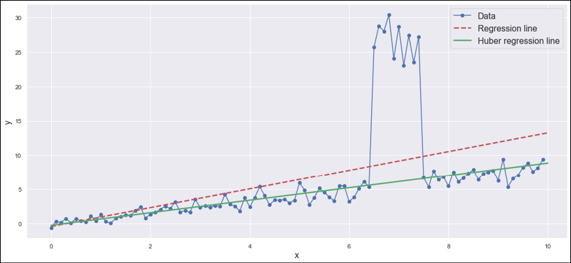
Comparison between standard linear regression and Huber regression

The diagram shows how negative the effect of the outliers might become when a simple linear regression is employed. Conversely, Huber loss keeps the regression line very close to the mean, with a minimum attraction by points that are about 10 times larger than the surrounding ones. Of course, the effect of is determinant; therefore, I invite the reader to repeat the exercise, changing this value and finding out the optimal trade-off when the set of outliers is larger.

Before moving on, it's helpful to remind ourselves how much R² can become dangerous when used without awareness. In this case, its value is larger for the linear regression because SSR is smaller when the slope gets closer to the outliers. The reason is simple: SSR is a quadratic measure, and 10 outliers whose magnitudes average 30 make a contribution that can easily overcome those of 70 inliers with an average equal to 5. In real-life cases, when the datasets are too complex to immediately identify the outliers, I suggest preprocessing the features using robust scaling. This will not affect the results, but avoids a situation where hidden outliers lead the model to a completely incorrect estimation.

Other regression techniques

A brief introduction to following regression techniques comes next, and why you may prefer to use them in comparison to least squares. In this section, we'll cover:

• Ridge regression, with a practical example in scikit-learn
• Lasso and logistic regression
• Polynomial regression with examples
• Isotonic regression

One of the most common problems with linear regression is the ill-conditioning that causes instabilities in the solution. Ridge regression has been introduced to overcome this problem.

Ridge Regression

A very common problem in regression models arises as a result of the structure of X^TX. We have previously shown that the presence of multi-collinearities forces , and this implies that the inversion becomes extremely problematic. A simple way to check the presence of multi-collinearities is based on the computation of the condition number of X^TX (with normalized columns with a length equal to 1), defined as:

In the previous formula, and ) are the largest and smallest singular values of X^TX, respectively. As X^TX is positive definite, its eigenvalues, , are positive and the singular values, which are equal to , are always defined. A small is associated with a well-conditioned problem, hence the inversion is not problematic. On the contrary, when , the problem is ill-posed, and the result can change dramatically following small variations in X.

A very simple and effective way to solve this problem is to employ a ridge (or Tikhonov) regularization, based on the L₂ norm of the parameter vector. Considering homoscedastic noise, the least-squares cost function becomes equal to:

The parameter determines the strength of the regularization and its role is immediately clear when considering the solution:

In the context of a ridge regression, we need to invert , which can be made non-singular even when X^TX is singular. Moreover, as is added to all diagonal elements, the resulting coefficients will be shrunk (the first term is like the denominator in a division). The larger is, the larger the amount of shrinkage obtained. As discussed in Chapter 1, Machine Learning Models Fundamentals, ridge regularization plays a fundamental role in preventing overfitting, but, in the context of linear regression, its main effect is to bias the model in order to lower the variance. We explained the concept of bias-variance trade-off earlier in this chapter, and this is a clear example of its necessity. Moreover, since X^TX is proportional to the covariance matrix, Cov[X], and is constant, its effect will be stronger on low-variance components. Therefore, ridge performs a minimal feature selection by shrinking the coefficients more when they're associated with less explicative features.

Example of Ridge Regression with scikit-learn

Let's now employ scikit-learn to evaluate the effect of ridge regression with the Diabetes dataset included in scikit-learn. The dataset contains 442 observations of male and female diabetic patients with information about age, body-mass index (BMI), and different blood pressure measures (average and 6 additional measures). The output is a numeric indicator regarding the progression of the disease. Without any further information, we can assume that the entries represent different patients and time is not included (for example, a different dataset might contain multiple entries for the same patients corresponding to different time periods). Hence, we want to check whether a linear regression can successfully fit the data.

The first step is to load the data and compute the condition number (the columns are already normalized):

import numpy as np

from sklearn.datasets import load_diabetes

data = load_diabetes()
X = data['data']
Y = data['target']

XTX = np.linalg.inv(X.T @ X)
print("k = {:.2f}".format(np.linalg.cond(XTX)))

The output of the previous snippet is:

k = 470.09

This value is extremely large, and indicates the presence of multi-collinearity. For our purposes, this result could be enough to proceed using a ridge regression, but as we want to perform a complete investigation, we want also to compute the Pearson correlation coefficients between the features. The elements of the resulting matrix, , are as follows:

Every coefficient with a clear meaning:

• If the i^th feature of X is positively correlated with the j^th feature of X, R_ij > 0.
• Analogously, if the i^th feature of X is negatively correlated with the j^th feature of X, R_ij > 0.
• R_ij = 0 if the two features are completely uncorrelated.

Of course, when the absolute value | R_ij | is close to 1, we can conclude that two features are correlated, and the problem is consequently ill-posed. A reasonable threshold depends on the specific context. However, a value | R_ij | > 0.5 should be considered carefully.

To have a better insight, let's compute the correlation matrix:

cm = np.corrcoef(X.T)

The output as a heatmap is shown in the following diagram:

Correlation matrix for the Diabetes dataset

It should be noted immediately that there are different large correlations, in particular, between blood pressure values (this is not surprising, considering that these patients monitor their blood pressure regularly). At this point, we can decide to proceed in different ways:

• Evaluating a ridge regression
• Removing the correlated features (keeping only one of the members of each couple)
• Choosing another regression strategy

As we're going to see, a simple linear regression is not very effective. Therefore, it's necessary to adopt a more complex method. However, it's helpful to evaluate the benefits of employing an L₂ penalty.

As a first step, let's perform CV using the RidgeCV class and the default R² score to find the optimal coefficient in the range (0.1, 1.0):

from sklearn.linear_model import RidgeCV

rcv = RidgeCV(alphas=np.arange(0.1, 1.0, 0.01),
              normalize=True)
rcv.fit(X, Y)

print("Alpha: {:.2f}".format(rcv.alpha_))

The output of the previous snippet is:

Alpha: 0.10

The CV grid search established that the smallest yields the best R² score. However, we know that ridge regression exacerbates the bias; therefore, we can check the condition number corresponding, for example, to :

print("k(0.1): {:.2f}".format(
        np.linalg.cond(X.T @ X + 
                       0.1 * np.eye(X.shape[1]))))
print("k(0.25): {:.2f}".format(
        np.linalg.cond(X.T @ X + 
                       0.25 * np.eye(X.shape[1]))))
print("k(0.5): {:.2f}".format(
        np.linalg.cond(X.T @ X + 
                       0.5 * np.eye(X.shape[1]))))

The output is as follows:

k(0.1): 37.99
k(0.25): 16.53
k(0.5): 8.90

The condition numbers are definitely much better than before. As the value corresponding to is a good trade-off between penalization (in other words, bias) and variance, we can pick this choice instead of 0.1 and evaluate the ridge regression using both R² and the MAE:

from sklearn.linear_model import Ridge
from sklearn.metrics import r2_score, mean_absolute_error

lrr = Ridge(alpha=0.25, normalize=True,
                random_state=1000)
lrr.fit(X, Y)

print("R2 = {:.2f}".format(
        r2_score(Y, lrr.predict(X))))
print("MAE = {:.2f}".format(
        mean_absolute_error(Y, lrr.predict(X))))

The output is as follows:

R2 = 0.50
MAE = 44.26

Unfortunately, the performances are not excellent. In particular, the output Y has and . Therefore, an MAE equal to about 44 could be problematic. The R² score confirms that the regression is able to explain only a fraction of total variation and, moreover, different parameter choices yield minimum changes. Therefore, this is a good point when introducing a trick that brings the power of non-linear models to GLMs given a sufficiently large sample size.

Risk modeling with Lasso and Logistic Regression

Ridge regression produces a global parameter shrinkage, but, as shown in Chapter 1, Machine Learning Models Fundamentals, the constraint surface is a hypersphere centered at the origin. Independent from the dimensionality, it is smooth, and this prevents the parameters from becoming null.

On the other hand, an L₁ penalty has the advantage of performing an automatic feature selection, because the smallest weights are pushed toward an edge of the constraint hypercube. Lasso regression is formally equivalent to ridge, but it employs L₁ instead of L₂:

The parameter controls the strength of the regularization, which, in this case, corresponds to the percentage of parameters that are forced to become equal to zero. Lasso regression shares many of the properties of ridge, but its main application is feature selection. In particular, given that a linear model has a large number of parameters, we can consider the association:

When m >> 1 and all coefficients are different from zero, it's quite difficult to understand which causes are dominant and whether some contributions cancel out one another. Such a situation leads the model to be poorly explainable and, consequently, less helpful in contexts (for example, healthcare) where a study of the causes is necessary. Lasso regression helps to solve this problem without the need for any external intervention. In fact, one simple strategy might be manually removing some features that a domain expert considers secondary or not correlated to the effect. However, this operation can be long and prone to become biased by human beliefs. Automatic feature selection, on the other hand, acts on the single parameters without any prior piece of information and it's much easier to check whether the result is reasonable from a domain viewpoint because the parameter set is much smaller.

In this example, we want to employ a lasso logistic regression to model a risk, establishing also the dominant factors. Before discussing the application, let's recap the main ideas behind logistic regression. Suppose that we have a binary random variable describing the risk we want to model (the outcome risk = 1 indicates the presence of a risk and, analogously, risk = 0 indicates the absence of a risk). The algorithm is based on the linear description of the logit, which is the logarithm of the odd ratio:

The logit must be non-negative and monotonically increasing. A function that satisfies this requirement is the sigmoid, . In fact, modeling P(risk = 1) with , which is defined on and whose values , we obtain the following:

Manipulating the logit expression, we get the required confirmation:

If we assume that all data points are i.i.d, we can model the log-likelihood as:

The last term is a binary version of the cross-entropy between the distribution of the true labels, p(y), and the predicted ones, q(y):

As , if y_i = 0, the first term , while the second one becomes equal to . Conversely, when y_i = 1, the second term is null, and the first is equal to . In both cases, the maximization of L forces the model to learn the actual distribution p(y). If we explicit the dependence of the parameter vector and introduce a generic penalty term, L becomes:

When the p-norm is L₁, the model will perform a lasso feature selection while modeling the odd ratio.

We can now model the risk of breast cancer using Python and scikit-learn.

Example of Risk modeling with Lasso and Logistic Regression

Let's now consider a toy example based on the Breast Cancer dataset, which contains 569 data points with 30 biological features. Each point is associated with a binary label, . As this is only an exercise, we don't consider the real medical requirements for such kinds of studies (readers who are interested in the topic should read a book on epidemiology). However, as the true labels are guaranteed by medical experts, if a logistic regression succeeds in successfully classifying the sample (with a reasonable accuracy), the logit of the risk will also be correct.

Let's start by loading and normalizing the dataset using a robust scaler and the quantile range (15, 85) (the dataset is based on real-world evidence (RWE) and doesn't contain very noisy outliers):

from sklearn.datasets import load_breast_cancer
from sklearn.preprocessing import RobustScaler

data = load_breast_cancer()
X = data["data"]
Y = data["target"]

rs = RobustScaler(quantile_range=(15.0, 85.0))
X = rs.fit_transform(X)

At this point, we can evaluate the performances of a lasso logistic regression with (this choice has been made by testing the results corresponding to different values. I invite the reader to do the same as an exercise):

import joblib

from sklearn.linear_model import LogisticRegression
from sklearn.model_selection import cross_val_score
cvs = cross_val_score(
   LogisticRegression(C=0.1, penalty="l1", solver="saga",
                      max_iter=5000, random_state=1000),
        X, Y, cv=10, n_jobs=joblib.cpu_count())

print(cvs)

As it's possible to see, we have chosen to impose an L₁ penalty. Therefore, we expect to reduce the number of parameters from 31 (intercept and coefficients) to a much smaller value. The output of the previous snippet is as follows:

[0.98275862 0.94827586 0.94736842 0.98245614 0.96491228 0.98245614 0.92982456 0.98214286 0.98214286 0.94642857]

The results are clearly positive. The worst accuracy is about 93%, with a maximum of 98%. Therefore, we can train the model with the entire dataset and use it for future predictions (assuming, of course, that they come from the same data-generating process – for example, the measures are taken using the same kind of instrument).

Let's now train the model and check the coefficients:

lr = LogisticRegression(C=0.05, penalty="l1", 
                        solver="saga",
                        max_iter=5000, 
                        random_state=1000)
lr.fit(X, Y)

for i, p in enumerate(np.squeeze(lr.coef_)):
    print("{} = {:.2f}".format(data['feature_names'][i], p))

The output of the previous snippet is as follows:

mean radius = 0.00
mean texture = 0.00
mean perimeter = 0.00
mean area = 0.00
mean smoothness = 0.00
mean compactness = 0.00
mean concavity = 0.00
mean concave points = -0.97
mean symmetry = 0.00
mean fractal dimension = 0.00
radius error = 0.00
texture error = 0.00
perimeter error = 0.00
area error = -0.90
smoothness error = 0.00
compactness error = 0.00
concavity error = 0.00
concave points error = 0.00
symmetry error = 0.00
fractal dimension error = 0.00
worst radius = -0.81
worst texture = -0.95
worst perimeter = -1.66
worst area = -0.16
worst smoothness = -0.08
worst compactness = 0.00
worst concavity = 0.00
worst concave points = -1.75
worst symmetry = -0.34
worst fractal dimension = 0.00

There are only nine non-null coefficients (out of 30) that can be rearranged so as to define the full relationship. As the risk is inverted (malignant = 0), in order to be coherent with the standard meaning, we're also inverting the sign of all coefficients (the sigmoid is symmetric; therefore, this is equivalent to swapping the labels):

model = "logit(risk) = {:.2f}".format(-lr.intercept_[0])
for i, p in enumerate(np.squeeze(lr.coef_)):
if p != 0:
    model += " + ({:.2f}*{}) ".
    format(-p, data['feature_names'][i])

print("Model:
")
print(model)

The output of the previous snippet is:

Model:
logit(risk) = -1.64 + (0.97*mean concave points)  + (0.90*area error)  + (0.81*worst radius)  + (0.95*worst texture)  + (1.66*worst perimeter)  + (0.16*worst area)  + (0.08*worst smoothness)  + (1.75*worst concave points)  + (0.34*worst symmetry)

Such an expression is very simple and provides an immediate insight into the dominant factors. As it's possible to see, some redundant features have been discarded because their contribution is probably partially absorbed by other features (in other words, there are confounding factors). At this point, the model should also be evaluated by a domain expert to understand whether it can help to build a diagnostic algorithm. However, it should be clear to the reader how powerful a linear model can be when there's no need for the extra capacity provided by larger models.

As an exercise, I invite the reader to change the value of (C for scikit-learn) until the number of non-null parameters stabilizes. Moreover, the reader can also incorporate an L₂ penalty through the ElasticNet loss (refer to Chapter 1, Machine Learning Models Fundamentals) to reduce the effect of multicollinearities.

Polynomial Regression

Linear regression is a simple and powerful algorithm because it can be fit very quickly and offers a high level of interpretability. For example, we can write the relation:

Even a non-technician can immediately understand the role played by the factors influencing the risk. To be more concrete, let's imagine that for the dependent variable , both factors are non-negative and:

It's easy to observe that, while Factor_a can increment the risk, the presence of Factor_b can reduce it. Moreover, if Factor_b > 2.5 Factor_a, the negative effect of Factor_a is neutralized by Factor_b (in other words, the risk becomes negative).

Even if this situation is almost ideal, the reality is quite often non-linear and the price to pay when working with linear models is a loss in terms of accuracy. When such a trade-off is acceptable, linear models are still the first choice (the Occam's razor principle), but when they don't meet the minimum requirements, it's necessary to look for other solutions. A simple but powerful alternative is offered by polynomial expansions of linear datasets.

Let's suppose that we have the following linear model (excluding the noise term):

Each of the terms is a regressor and is obtained as a linear combination of all regressors. Indeed, we're including any constraint regarding the real nature of . They can be simple factors, but they can also be, for example, square factors, or products of different factors. For the sake of rigor, we need to admit that the noise term cannot be easily discarded and what we're explaining is only correct when has the same nature of the regressors. For example, if we exchange with , the noise contribution should also be squared, and the same happens for more complex transformations (such as log-linear models). However, in practice, we can often discard this control because we estimate the noise implicitly through the residuals and it's not always necessary to form confidence intervals (which rely on the distributional family of the noise). On the other hand, we know that the normality assumption can be relaxed when the sample size is large enough to justify application of the Central Limit Theorem; hence, we continue to employ the standard algorithms described in the previous section also when the distribution of each single noise term is no longer normal.

A polynomial regression is indeed a linear regression based on the transformation of the original feature set into its polynomial expansion. For example, a quadratic regression is obtained through the transformation:

Unfortunately, this kind of transformation is prone to explode when the initial dimensionality is large. In fact, considering both polynomial and interaction features, the total number grows exponentially because of all combinations of every degree. For example, transforming the Diabetes dataset (13 original features) with a degree of 3, we obtain 560 features, which exceed the sample size (506). The drawbacks are obvious:

• The sample size can become too small due to the curse of dimensionality (for example, CV becomes extremely problematic because the folds are too small, and some regions can be easily cut out from the training set).
• The estimator can now overfit (hence, ridge is preferred over a standard linear regression).
• Both computational and memory complexities grow very rapidly.

In these cases, we can try to mitigate the problem by selecting only the interaction features, but this choice would not help us in capturing the oscillations due to the non-linearities. However, in many real cases, the main problem is due to the inability to manage the interactions (for example, in a lot of healthcare studies, comorbidities – which means the presence of different, linked pathologies at the same time – play a central role and it's not possible to model the interaction effects as a linear combination). Therefore, when the complexity of the datasets is very large, I suggest starting by generating interaction-only features and checking whether the result is acceptable. In case of poor performances, it's possible either to increase the degree or activate the full feature set.

Another important element to consider is the use of CV. If the sample size is very small, a low number (for example, less than 10) of folds results in training sets that might not cover the whole data-generating process. Consequently, the validation results are generally poor. The only way to address this problem is to use a Leave-One-Out (LOO) (if it's possible to evaluate a metric on a single data point) or Leave-P-Out (LPO). Clearly, both strategies are extremely time consuming, but this is the only feasible way to manage CV effectively in these cases.

In any case, it's important to remember that K-fold CV is generally the most reliable choice because it avoids the cross-correlations that are almost inevitable with LOO and LPO. Alternatively, it's possible to perform a static train-test split after having shuffled the dataset properly. Obviously, the size of the test set must be small enough to allow the training set to capture the whole dynamic of p_data. If the regression is completely time-independent, a small training set might be large enough to train a model, but this problem can become very hard to manage when the data points are based on an evolution over time. In these cases, the exclusion of some points could lead to a biased model because of an under-estimation (or over-estimation) of the parameters.

Therefore, when working with time series, it's often preferable to employ specific models (which we're going to present in the next chapter) that are able to capture the internal dynamics and the interdependencies between time points. If a regression model is preferred, it's necessary to check whether the training set contains enough data points to describe the data-generating process.

Moreover, when working with polynomial regressions, the degrees of freedom, t, can be very large and, as generic rule of thumb, N >> t. If, on the contrary, or, even worse, N < t, the model is partially undetermined, and the performances could become poorer than the linear counterpart.

Examples of Polynomial Regressions

As a first example, let's see how a ridge regression can be adapted to manage a non-linear 1-dimensional dataset defined as:

We have also voluntarily included transformations of the noise terms to increase the complexity and we have also normalized the set, Y, to avoid a very large range:

import numpy as np

x = np.expand_dims(np.arange(-50, 50, 0.1), axis=1)
y = 0.1 * np.power(x + 
    np.random.normal(0.0, 2.5, size=x.shape), 3) + 
    3.0 * np.power(x - 2 +                       np.random.normal(0.0, 1.5, size=x.shape), 2) - 
    5.0 * (x + np.random.normal(0.0, 0.5, size=x.shape))

y = (y - np.min(y)) / (np.abs(np.min(y)) + np.max(y))

At this point, we can train a standard ridge model (with ):

from sklearn.linear_model import Ridge

lr = Ridge(alpha=0.1, normalize=True, random_state=1000)
lr.fit(x, y)

Before moving on and comparing the results, it's helpful to evaluate both R² and the MAE:

from sklearn.metrics import r2_score, mean_absolute_error
print("R2 = {:.2f}".format(
        r2_score(y, lr.predict(x))))
print("MAE = {:.2f}".format(
        mean_absolute_error(y, lr.predict(x))))

The output of the previous snippet is:

R2 = 0.63
MAE = 0.10

This result might appear surprising because the dataset is highly non-linear. Indeed, the reader must pay attention to two important factors. The values of ; therefore, we have about 10% of the MAE, which is generally too large for this kind of dataset. The reason will be clear when comparing the results, but generally speaking, the effect of the error is greater in the regions where the slope changes more abruptly. In this case, there are two such kinds of regions. The least squares algorithm successfully minimizes the error by selecting a slope that is more compatible with the first curved region and ineffective for the second one.

The second thing to remember is the informative value of R². As many authors have demonstrated, this score is very context-dependent and sometimes, it can also yield inconsistent results. In particular, R² must always be used in comparisons of compatible versions of a model (for example, the same dataset and different polynomial degrees), because it doesn't provide any information about the absolute goodness of fit. Moreover, it doesn't encode information about the turning points of polynomial curves. When working with linear regressions, this is not a problem. However, when using polynomial transformations, it's extremely important to understand whether the curve models the data correctly in its non-linear structure. A much more reliable alternative is provided by the U scores (also known as Theil scores), which are defined as:

The standard U score is very similar to R² and encodes information about the total variation that the model is able to describe. Instead, is based on stepwise differences and enables the ability of the model to be measured in turning on time. Looking at the numerator, the first term is the difference between two consecutive outputs, while the second one is the difference between the predicted output and the true previous one. An ideal model should be characterized by and, consequently, .

In fact, in this case, the turning points are successfully predicted, and the model follows the non-linear structure of the data. In real cases, we look for the hyperparameter set that minimizes both scores (possibly including also the adjusted R² in order to take into account the degrees of freedom and penalize more complex models).

As a first step, let's define a function to compute both U scores:

import numpy as np

def u_scores(y_true, y_pred):
    a = np.sum(np.power(y_true - y_pred, 2))
    b = np.sum(np.power(y_true, 2))
    u = np.sqrt(a / b)
    
    d_true = y_true[:y_true.shape[0]-1] - y_true[1:]
    d_pred = y_pred[:y_pred.shape[0]-1] - y_true[1:]
    c = np.sum(np.power(d_true - d_pred ,2))
    d = np.sum(np.power(d_true, 2))
    ud = np.sqrt(c / d)
    
    return u, ud

We can now check the values for a linear regression:

print("U = {:.2f}, UD = {:.2f}"
            .format(*u_scores(y, lr.predict(x))))

The output is as follows:

U = 0.37, UD = 3.38

Since U scores are also relative measures, we cannot draw any conclusion without comparing the results with a few polynomial regressions. Let's create three alternative datasets based on degrees 5, 3, and 2, including interactions using the PolynomialFeatures class:

from sklearn.preprocessing import PolynomialFeatures

pf5 = PolynomialFeatures(degree=5)
xp5 = pf5.fit_transform(x)

pf3 = PolynomialFeatures(degree=3)
xp3 = pf3.fit_transform(x)

pf2 = PolynomialFeatures(degree=2)
xp2 = pf2.fit_transform(x)

We can now fit the respective ridge regressions, keeping :

lrp5 = Ridge(alpha=0.1, normalize=True, random_state=1000)
lrp5.fit(xp5, y)
yp5 = lrp5.predict(xp5)

lrp3 = Ridge(alpha=0.1, normalize=True, random_state=1000)
lrp3.fit(xp3, y)
yp3 = lrp3.predict(xp3)

lrp2 = Ridge(alpha=0.1, normalize=True, random_state=1000)
lrp2.fit(xp2, y)
yp2 = lrp2.predict(xp2)

At this point, we can evaluate the U scores:

print("2. U = {:.2f}, UD = {:.2f}".
          format(*u_scores(y, yp2)))
print("3. U = {:.2f}, UD = {:.2f}".
          format(*u_scores(y, yp3)))
print("5. U = {:.2f}, UD = {:.2f}".
          format(*u_scores(y, yp5)))

The output of the previous snippet is:

2. U = 0.21, UD = 1.92
3. U = 0.10, UD = 0.93
5. U = 0.09, UD = 0.83

The results confirm our hypotheses. If we look at s, we already have a rapid decrease when the degree is 2, but the value seems to stabilize with d = 3. In fact, considering also the standard U score, there's a 50% drop between degree 2 and 3, while it remains almost constant for d = 5. This indicates that a degree 5 model is more prone to overfit, and the extra degrees of freedom are not to reduce the bias at the expense of the variance. In fact, the more complex model can explain the same variation, but it has more potential turning points that might be unnecessary.

The plot of all the models is shown in the following graph:

Non-linear noisy dataset overlaid with linear and three polynomial regressions

It's clear that a linear regression (dashed line) is totally inaccurate and should be excluded immediately. Assuming the structure of the dataset, the degree 2 polynomial is not a good choice either because it doesn't allow any saddle point. Looking at the dataset, there's a saddle point for (the concavity changes direction) and the parabolic regression can only capture a side of the curve. Both degrees 3 and 5 are odd; therefore, they allow the concavity direction change and, indeed, the two curves almost overlap (with a slightly more precise prediction ability for d = 5).

However, the cost of the extra complexity is not justified by the results. Therefore, we prefer to employ a degree three model. Moreover, it's important to remember that the dataset should represent the entire data-generating process. In this particular case, it means that, when x < –40 and x > 60, the trend remains the same. This implies that , which is clearly unrealistic in most actual cases. Hence, we're explicitly assuming that the independent variable, x, has a limited domain, which is fully captured by the training sample.

Returning to the Diabetes dataset, the U scores corresponding to a ridge regression with are as follows:

U = 0.32, UD = 0.51

These values don't seem too bad, but we know that R² = 0.5, and so we haven't achieved a high goodness of fit. We can test the effect of using polynomial features, but we also have to pay attention to the sample size. The original dataset contains 506 points with 13 features; therefore, the expansion must be limited, otherwise we risk having an undetermined system. Considering the nature of the dataset, it's reasonable to suppose that the lack of precision is mainly due to the inability to model the interactions between factors (this is a common scenario in healthcare studies). Therefore, we can limit the expansion to d = 3, including just the interactions:

pf = PolynomialFeatures(degree=3, interaction_only=True)
Xp = pf.fit_transform(X)

This transformation generates 176 features, fewer than the sample size, but it's still a very large number corresponding to a data-generating process that might not be fully captured by 506 points. However, we can retrain the ridge regression and compute the new measures:

lrr = Ridge(alpha=0.25, normalize=True,random_state=1000)
lrr.fit(Xp, Y)

print("R2 = {:.2f}".format(r2_score(Y, lrr.predict(Xp))))
print("MAE = {:.2f}".
       format(mean_absolute_error(Y, lrr.predict(Xp))))
    
print("U = {:.2f}, UD = {:.2f}".
format(*u_scores(Y, lrr.predict(Xp))))

The output is as follows:

R2 = 0.60
MAE = 39.24
U = 0.29, UD = 0.46

All the measures confirm an improvement, but it's obvious that a larger sample size could yield a much better fit. In particular, the reduction of indicates that the polynomial model is now capturing more turning points (a result that is also confirmed by the lower MAE). Unfortunately, all other combinations with higher degrees yield a total number of features larger than the training sample; therefore, they are not acceptable. Anyhow, it must be clear that polynomial regression is an extremely powerful tool for managing problems that are either naturally non-linear or with dependent features.

As an exercise, I invite the reader to test these models with other simple regression datasets, such as the Boston house pricing dataset, trying to establish the optimal trade-off between accuracy, degree, and the number of generated features.

Isotonic Regression

In some cases, the dataset is made up of a sample of a monotonic function . A standard linear regression can easily capture the slope, but it fails when the curve is non-linear. On the other hand, polynomial regressions can also capture non-linear dynamics, but the models can easily become too complex because of the necessity of high degrees. Moreover, the boundary conditions cannot be easily managed, and the resulting regression will diverge to when . An isotonic regression assumes the monotonicity of the dependent variable and tries to find a set of N weights, w_i, so as to minimize the weighted least-square loss:

The resulting function is an actual constrained interpolation of the points {(x₁, y₁), (x₂, y₂), …, (xN, yN)} and cannot generally be expressed as linear combination of the independent variables. The main advantage is that even complex non-linear dynamics with several slope changes can be easily captured. However, when the dataset is very noisy, the interpolation might become overfitted. To address this problem (and all related ones), it's possible to smooth the dataset before processing it, as discussed in the following section. For now, let's suppose that the noise is controlled, and we prefer a piecewise interpolation to a coarse approximation.

Example of Isotonic Regression

As an example, let's consider a dataset containing 600 points, where (this is the only condition required by an isotonic regression):

import numpy as np

x = np.arange(0, 60, 0.1)
y = 0.1 * np.power(x + np.random.normal(0.0, 1.0, size=x.shape), 3) + 
  3.0 * np.power(
  x - 2 + np.random.normal(0.0, 0.5, size=x.shape), 2) - 
  5.0 * (x + np.random.normal(0.0, 0.5, size=x.shape))

y = (y - np.min(y)) / (np.abs(np.min(y)) + np.max(y))

To have an immediate comparison, let's fit both a standard linear regression and an isotonic one:

from sklearn.linear_model import LinearRegression
from sklearn.isotonic import IsotonicRegression

lr = LinearRegression()
lr.fit(np.expand_dims(x, axis=1), y)

ir = IsotonicRegression()
ir.fit(x, y)

The result is shown in the following diagram:

Linear regression compared to isotonic regression

The inner structure of the dataset is parabolic, and we could have been tempted to use a polynomial regression with degree 2. However, such a solution wouldn't capture the sub-dynamics due to noise, and this can be either positive or negative. As we have chosen to trust the noisy oscillations, the isotonic regression yielded an optimal result using a piecewise interpolation that minimizes the mean square error.

As an exercise, I invite the reader to compare the results (in terms of error) with a polynomial regression and select the model that best describes the underlying data-generating process (with and without noise).

Summary

In this chapter, we have introduced the reader to the most important concepts concerning linear models and regressions. In the first part, we discussed the features of a GLM, focusing attention on how to fit the models and how to avoid the most common problems.

We also analyzed how to include regularization penalties through ridge and lasso regressions and how it's possible to exploit the linear framework also when the dataset is non-linear through an appropriate polynomial transformation. We also compared the results with the one obtained using an isotonic regression and we analyzed the reasons for preferring either the former or the latter. Another important topic discussed in the chapter is risk modeling using logistic regression penalized with lasso to perform an automatic feature selection.

In the next chapter, we start discussing the basic concepts and of time-series analysis, focusing on the properties on the most important models (ARMA and ARIMA) that are commonly employed in econometrics and financial forecasting.

Further reading

• Greene W. H., Econometric Analysis (Fifth Edition), Prentice Hall, 2002
• Belsley D. A., Kuh E., Welsch R., Regression Diagnostics: Identifying Influential Data and Sources of Collinearity, Wiley, 1980
• Chakravarti N., Isotonic Median Regression: A Linear Programming Approach, Mathematics of Operations Research, 14/2, 1989
• Candanedo L. M., Feldheim V., Deramaix D., Data-Driven Prediction Models of Energy Use of Appliances in a Low-Energy House, Energy and Buildings, Volume 140, 04/2017