21

Autoencoders

In this chapter, we're going to look at an unsupervised model family whose performance has been boosted by modern deep learning techniques. Autoencoders offer a different approach to classic problems such as dimensionality reduction or dictionary learning; however, unlike many other algorithms, they don't suffer the capacity limitations that affect many famous models. Moreover, they can exploit specific neural layers (such as convolutions) to extract pieces of information based on specialized criteria. In this way, the internal representations can be more robust to different kinds of distortion, and much more efficient in terms of the amount of information they can process.

In particular, we will discuss the following:

• Standard autoencoders
• Denoising autoencoders
• Sparse autoencoders
• Variational autoencoders

We can now start discussing the main concepts of autoencoders, focusing on the structural components and their features. In the next sections, we're going to further expand these concepts in order to solve more complex problems.

Autoencoders

In the previous chapters (in particular, Chapter 3, Introduction to Semi-Supervised Learning and Chapter 4, Advanced Semi-Supervised Classification on semi-supervised learning), we discussed how real datasets are very often high-dimensional representations of samples that lie on low-dimensional manifolds (this is one of the semi-supervised pattern's assumptions, but it's generally true).

As the complexity of a model is proportional to the dimensionality of the input data, many techniques have been analyzed and optimized in order to reduce the actual number of valid components. For example, PCA selects features according to their relative explained variance, while ICA and generic dictionary learning techniques look for basic atoms that can be combined to rebuild the original samples. In this chapter, we're going to analyze a family of models based on a slightly different approach, but whose capabilities are dramatically increased by the employment of deep learning methods. A generic autoencoder is a model that is split into two separate (but not completely autonomous) components called an encoder and a decoder. The task of the encoder is to transform an input sample into an encoded feature vector, while the task of the decoder is the opposite: rebuilding the original sample using the feature vector as input. The following diagram shows a schematic representation of a generic model:

Schema of a generic autoencoder

More formally, we can describe the encoder as a parametrized function:

The output is a vectorial code whose dimensionality is normally quite a bit lower than the input's dimensionality. Analogously, the decoder is described as follows:

The goal of a standard algorithm is to minimize a cost function that is proportional to the reconstruction error. A classic method is based on the mean squared error (MSE) (working on a dataset with a sample size equal to M):

This function depends only on the input samples (which are constant) and the parameter vectors; therefore, this is a de facto unsupervised method where we can control the internal structure and the constraints imposed on the code. From a probabilistic viewpoint, if the input samples are drawn from a p(X) data-generating process, our goal is to find a q(X) parametric distribution that minimizes the Kullback–Leibler divergence with p(X). Considering the previous definitions, we can define a conditional distribution as follows:

Therefore, the Kullback–Leibler divergence becomes the following:

The first term represents the negative entropy of the original distribution, which is constant and isn't involved in the optimization process. The second term is the cross entropy between p and q. If we assume Gaussian distributions for p and q, the MSE is proportional to the cross entropy (for optimization purposes, it's equivalent to it), and therefore this cost function is still valid under a probabilistic approach. Alternatively, it's possible to consider Bernoulli distributions for p and q, and the cross entropy becomes the following:

The main difference between the two approaches is that while an MSE can be applied to (or multidimensional matrices), Bernoulli distributions need (formally, this condition should be ; however, the optimization can also be performed successfully when the values are not binary). The same constraint is necessary for the reconstructions; therefore, when using neural networks, the most common choice is to employ sigmoid layers. To be precise, if the data-generating process is assumed to be Gaussian, the cross entropy becomes the MSE. I invite you to check this, but the calculation is extremely easy because we have:

Excluding the terms not subject to optimization, it's straightforward to understand that the actual cross entropy between the original distribution and the autoencoder distribution is indeed equivalent to an MSE cost function.

Example of a deep convolutional autoencoder with TensorFlow

This example (like all the others in this and the following chapters) is based on TensorFlow 2.0 (for information about the installation of TensorFlow, please refer to the information provided on the official page: https://www.tensorflow.org/). As explained in the previous chapters, TensorFlow has evolved to incorporate Keras and offers extraordinary flexibility in creating and training deep models. We'll approach this example pragmatically, which means we won't explore all the features; they're beyond the scope of this book. However, interested readers can refer to the book Holdroyd T., TensorFlow 2.0 Quick Start Guide, Packt Publishing, 2019.

In this example, we are going to create a deep convolutional autoencoder and train it using the Fashion MNIST dataset. The first step is loading the data (using the Keras helper function), normalizing the data, and, in order to speed up the computation, limiting the training set to 1,000 data points:

import tensorflow as tf
import numpy as np
nb_samples = 1000
nb_epochs = 400
batch_size = 200
code_length = 256
(X_train, _), (_, _) = 
        tf.keras.datasets.fashion_mnist.load_data()
X_train = X_train.astype(np.float32)[0:nb_samples] 
              / 255.0
width = X_train.shape[1]
height = X_train.shape[2]
X_train_g = tf.data.Dataset.
   from_tensor_slices(np.expand_dims(X_train, axis=3)).
   shuffle(1000).batch(batch_size)

The generator X_train_g is based on the utility class Dataset provided by TensorFlow 2.0. It allows you to select the block of data needed for training and testing purposes (in our case, there's no test generator), automatically shuffle it (to remove potential collinearities), and return batches at every call.

At this point, we can create a class inheriting from tf.keras.Model, setting up the whole architecture, which is made up of the following:

The encoder (all layers have padding "same" and ReLU activation):

• Convolution with 32 filters, kernel size equal to (3 × 3), and strides (2 × 2)
• Convolution with 64 filters, kernel size equal to (3 × 3), and strides (1× 1)
• Convolution with 128 filters, kernel size equal to (3 × 3), and strides (1 × 1)

The decoder:

• Transpose convolution with 128 filters, kernel size equal to (3 × 3), and strides (2 × 2)
• Transpose convolution with 64 filters, kernel size equal to (3 × 3), and strides (1× 1)
• Transpose convolution with 32 filters, kernel size equal to (3 × 3), and strides (1 × 1)
• Transpose convolution with 1 filter, kernel size equal to (3 × 3), strides (1 × 1), and a sigmoid activation

As the images are (28 x 28), it makes things easier for us if we resize each batch to have dimensions of (32 x 32), to easily manage all of the subsequent operations that are based on sizes that are a power of 2.

The encoder performs a series of convolutions, starting with larger strides (2 x 2) to capture high-level features and proceeds with 64 and 128 convolutions with (1 x 1) strides to learn more and more detailed features. As explained in Chapter 19, Deep Convolutional Networks, convolutions work in a sequential fashion, therefore, a standard architecture generally follows a hierarchical sequence, with a few top-level convolutions and more low-level ones. In this case, the size of the images is very small, and therefore it's a good idea to keep (3 x 3) kernels through the encoder network. In the case of larger images, instead, the first convolutions should also involve larger kernels, while the last ones must focus on smaller details and the size should be smaller (the normal minimum value is (2 x 2)).

The decoder has a symmetric architecture because it's based on transpose convolutions (that is, deconvolutions). Therefore, once the code is reshaped, the first filters have to work with detailed features, while the last ones must generally focus on high-level elements (for example, borders). The last transpose convolution is responsible for building the output, which must match the input size. Since we're working with grayscale images in our example, we're employing a single filter, while RGB images require three filters. A practical discussion can be had about the strides. When the networks have a very large capacity, it's possible to use the strides to adjust the output of a transpose convolution layer (multiplying each dimension by the corresponding stride value) in order to match the final desired dimensions. This can be a clever trick to add further convolutions (or to remove them) without altering the output. Instead, if the reconstructions' quality doesn't meet the expected requirements, it's sometimes preferable to resize the images using a specialized high-order function (like we do in the input phase). Your choice must be made by evaluating the MSE and, if possible, also through a visual inspection of the results.

TensorFlow 2.0, when working with classes derived from tf.keras.Model, requires the definition of the variables in the constructor, while the methods are free to manipulate them to obtain specific results. In our case, we have:

• The constructor, with all layers required for both the encoder and the decoder
• The encoder method
• The decoder method
• The resizing method as a utility function
• The overload of the call() method to invoke the main operation directly using the model instance:

  class DAC(tf.keras.Model):
      def __init__(self):
          super(DAC, self).__init__()
          # Encoder layers
          self.c1 = tf.keras.layers.Conv2D(
              filters=32,
              kernel_size=(3, 3),
              strides=(2, 2),
              activation=tf.keras.activations.relu,
              padding='same')
          self.c2 = tf.keras.layers.Conv2D(
              filters=64,
              kernel_size=(3, 3),
              activation=tf.keras.activations.relu,
              padding='same')
          self.c3 = tf.keras.layers.Conv2D(
              filters=128,
              kernel_size=(3, 3),
              activation=tf.keras.activations.relu,
              padding='same')
          self.flatten = tf.keras.layers.Flatten()
          self.dense = tf.keras.layers.Dense(
              units=code_length,
              activation=tf.keras.activations.sigmoid)
          # Decoder layers
          self.dc0 = tf.keras.layers.Conv2DTranspose(
              filters=128,
              kernel_size=(3, 3),
              strides=(2, 2),
              activation=tf.keras.activations.relu,
              padding='same')
          self.dc1 = tf.keras.layers.Conv2DTranspose(
              filters=64,
              kernel_size=(3, 3),
              activation=tf.keras.activations.relu,
              padding='same')
          self.dc2 = tf.keras.layers.Conv2DTranspose(
              filters=32,
              kernel_size=(3, 3),
              activation=tf.keras.activations.relu,
              padding='same')
          self.dc3 = tf.keras.layers.Conv2DTranspose(
              filters=1,
              kernel_size=(3, 3),
              activation=tf.keras.activations.sigmoid,
              padding='same')
      def r_images(self, x):
          return tf.image.resize(x, (32, 32))
      def encoder(self, x):
          c1 = self.c1(self.r_images(x))
          c2 = self.c2(c1)
          c3 = self.c3(c2)
          code_input = self.flatten(c3)
          z = self.dense(code_input)
          return z
      def decoder(self, z):
          decoder_input = tf.reshape(z, (-1, 16, 16, 1))
          dc0 = self.dc0(decoder_input)
          dc1 = self.dc1(dc0)
          dc2 = self.dc2(dc1)
          dc3 = self.dc3(dc2)
          return dc3
      def call(self, x):
          code = self.encoder(x)
          xhat = self.decoder(code)
          return xhat
  model = DAC()
  

Once we have also defined an instance of our class (called model for simplicity), we can define the optimizer, which is Adam with :

optimizer = tf.keras.optimizers.Adam(0.001)

The next step consists of defining a helper function to collect information about the training loss. In our case, it's enough to compute the mean of the loss function over each batch:

train_loss = tf.keras.metrics.Mean(name='train_loss')

Now we need to create the training function, which is one of the innovations introduced in TensorFlow 2.0. Let's define it first:

@tf.function
def train(images):
    with tf.GradientTape() as tape:
        reconstructions = model(images)
        loss = tf.keras.losses.MSE(
            model.r_images(images), reconstructions)
    gradients = tape.gradient(
        loss, model.trainable_variables)
    optimizer.apply_gradients(
        zip(gradients, model.trainable_variables))
    train_loss(loss)

This function is marked with a decorator that informs TensorFlow that it's going to work with the variables defined in the model. To apply the backpropagation algorithm, we need to perform the following steps:

• Activate a GradientTape context that will take care of computing the gradients of all trainable variables.
• Run the model (the feed-forward phase).
• Evaluate the loss function (in our case, it's a standard mean square error).
• Compute the gradients.
• Ask the optimizer to apply the gradients to all trainable variables (of course, each algorithm performs all the necessary additional operations).
• Accumulate the training loss.

The corresponding Python commands are straightforward and only a little different from the previous TensorFlow versions. Once this function has been declared, it's possible to start the training process:

for e in range(nb_epochs):
    for xi in X_train_g:
        train(xi)
    print("Epoch {}: Loss: {:.3f}".
          format(e+1, train_loss.result()))
    train_loss.reset_states()

The output of the previous snippet is:

Epoch 1: Loss: 0.136
Epoch 2: Loss: 0.090
…
Epoch 399: Loss: 0.001
Epoch 400: Loss: 0.001

Hence, at the end of the training process, the average mean square error is 0.001. Considering that the images are resized to 32 x 32 and the values are in the range (0,1), the mean absolute error (MAE) ranges between 0 and 1,024. Therefore, an error equal to 0.001 guarantees a high reconstruction quality (it's equivalent to an MAE that is equal to about 0.03 or 3% of the maximum error) of about 97%. Whenever the MSE is considered a reliable reconstruction metric, this approach can also be generalized to data points different from images.

It's also interesting to analyze the length of the code (for instance, the encoder output). As it's standardized in the range (0,1), a total average close to 0.5 indicates that about 50% of the values are active, while the remaining ones are close to 0 (without taking into account the standard deviation). A value slightly larger than 0.5 indicates that the code is very dense, while a value slightly lower than 0.5 is a sign of sparsity because more than 50% of the units have a very low activation:

codes = model.encoder(np.expand_dims(X_train, axis=3))
print("Code mean: {:.3f}".format(np.mean(codes)))
print("Code STD: {:.3f}".format(np.std(codes)))

The output of the previous block is:

Code mean: 0.554
Code STD: 0.241

As expected (considering that we haven't imposed any constraints), our code is moderately dense. This also means that it's not generally possible to drastically reduce the code length (in the example, it was set equal to 256) without a significant loss of information. The reason for this is directly connected to the entropy of the code. For example, in the case of two images, we know that the optimal encoding requires a single binary unit; however, with complex images, we should consider the full joint probability distribution to estimate the optimal length, and this is generally intractable. Therefore, a good strategy is to start with a length of about of the dimensionality and to proceed by reducing it until the mean square error remains below a fixed threshold. It goes without saying that a part of the information managed by an autoencoder is stored in the weights of the model; hence, a deeper architecture is normally able to manage shorter code, while a very shallow network requires more information in the code.

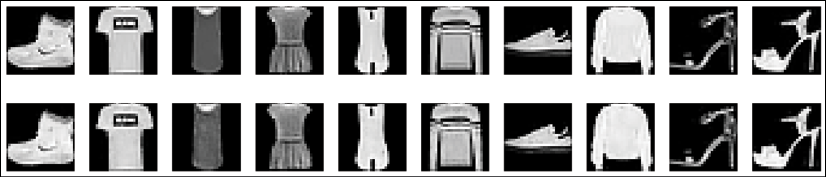
We can now visualize some original images and their reconstructions:

Original images (first row) and their reconstructions (second row)

We can see how the loss of information is limited to secondary details and the autoencoder has successfully learned how to reduce the dimensionality of the input samples.

As an exercise, I invite the reader to split the code into two separate sections (encoder and decoder) and to optimize the architecture in order to achieve better accuracy on the whole Fashion MNIST dataset.

Denoising autoencoders

Autoencoders can be used to determine under-complete representations of a dataset. However, Bengio et al. (in Vincent P., Larochelle H., Lajoie I., Bengio Y., Manzagol P., Stacked Denoising Autoencoders: Learning Useful Representations in a Deep Network with a Local Denoising Criterion, from the Journal of Machine Learning Research, 11/2010) proposed using autoencoders to denoise the input samples rather than learning the exact representation of a sample in order to rebuild it from low-dimensional code.

This is not a brand-new idea, because, for example, Hopfield networks (proposed a few decades ago) had the same purpose, but their limitations in terms of capacity led researchers to look for different methods. Nowadays, deep autoencoders can easily manage high-dimensional data (such as images) with a consequent space requirement. That's why many people are now reconsidering the idea of teaching a network how to rebuild a sample image starting from a corrupted one. Formally, there are not many differences between denoising autoencoders and standard autoencoders. However, in this case, the encoder must work with noisy samples:

The decoder's cost function remains the same. If the noise is sampled for each batch, repeating the process for a sufficiently large number of iterations allows the autoencoder to learn how to rebuild the original image when some fragments are missing or corrupted. To achieve this goal, the authors suggested different possible kinds of noise. The most common choice is to sample Gaussian noise, which has some helpful features and is coherent with many real-world noisy processes:

Another possibility is to employ an input dropout layer, zeroing some random elements:

This choice is clearly more drastic, and the rate must be properly tuned. A very large number of dropped pixels can irreversibly delete many pieces of information and the reconstruction can become more difficult and rigid (our purpose is to extend the autoencoder's ability to other samples drawn from the same distribution). Alternatively, it's possible to mix up the Gaussian noise and the dropout's, switching between them with a fixed probability. Clearly, the models must be more complex than standard autoencoders because now they have to cope with missing information.

The same concept applies to the code length: very under-complete code wouldn't be able to provide all the elements needed to reconstruct the original image in the most accurate way. I suggest testing all the possibilities, in particular when the noise is constrained by external conditions (for example, old photos or messages transmitted through channels affected by precise noise processes). If the model must also be employed for never-before-seen samples, it's extremely important to select samples that represent the true distribution, using data augmentation techniques (limited to operations compatible with the specific problem) whenever the number of elements is not enough to reach the desired level of accuracy.

Example of a denoising autoencoder with TensorFlow

This example doesn't require any dramatic modification of the model previously defined. In fact, the denoising ability is an intrinsic property that every autoencoder has. In order to test it, we only need to consider that the training function now needs both the noisy images and the original ones:

model = DAC()
@tf.function
def train(noisy_images, images):
    with tf.GradientTape() as tape:
        reconstructions = model(noisy_images)
        loss = tf.keras.losses.MSE(
            model.r_images(images), reconstructions)
    gradients = tape.gradient(
        loss, model.trainable_variables)
    optimizer.apply_gradients(
        zip(gradients, model.trainable_variables))
    train_loss(loss)

As it's possible to see, the mean square error is now computed between the reconstructions and the original images (which are not the input of the model anymore), while the model is fed with the noisy images. If the noise is randomly sampled at each training step, the autoencoder learns the structure of the manifold where the data lies and, at the same time, it becomes robust to small variations of the input. This result is a consequence of the smoothness assumption (see Chapter 3, Introduction to Semi-Supervised Learning) and of the fact that the mean of a set of corrupted data points defines an attractor basin. Hence, the noisy input yields slightly different code that is decoded as the closest mean. Of course, if the variation is too large, considering the high non-linearity of the model, the probability of recovering the original image becomes smaller and smaller. For our purposes, we are going to consider clipped Gaussian noise:

In this way, the noisy images are always implicitly normalized, assuming values in the range (0,1):

for e in range(nb_epochs):
        for xi in X_train_g:
            xn = np.clip(xi +
                  np.random.normal(
                   0.0, 0.2,
                   size=(batch_size, width, height, 1)),
                  0.0, 1.0)
            train(xn, xi)
        print("Epoch {}: Loss: {:.3f}".
              format(e + 1, train_loss.result()))
        train_loss.reset_states()

The output of the previous snippet is:

Epoch 1: Loss: 0.146
Epoch 2: Loss: 0.100
…
Epoch 399: Loss: 0.002
Epoch 400: Loss: 0.002

Considering the capacity of these models, it's not surprising to see that the final loss is almost the same as a standard autoencoder. Therefore, we can be sure that any noisy image (based on clipped Gaussian noise with the unit variance/identity covariance matrix) will be correctly recovered.

We can see some examples in the following figure:

Noisy images (first row) and their reconstructions (second row)

The denoising autoencoder has successfully learned to rebuild the original images (with an MAE equal to about 0.04 and, therefore, an accuracy of about 96%) in the presence of Gaussian noise. I invite you to test other methods (such as using an initial dropout) and increase the noise level to understand what the maximum corruption is that this model can effectively remove.

Sparse autoencoders

In general, standard autoencoders produce dense internal representations. This means that most of the values are different from zero. In some cases, however, it's more useful to have sparse code that can better represent the atoms belonging to a dictionary. In this case, if , , we can consider each sample as the overlap of specific atoms weighted accordingly. To achieve this objective, we can simply apply an L₁ penalty to the code layer, as explained in Chapter 2, Loss functions and Regularization. The loss function for a single sample, therefore, becomes the following:

In this case, we need to consider the extra hyperparameter α, which must be tuned to increase the sparsity without a negative impact on the accuracy. As a general rule of thumb, I suggest starting with a value equal to 0.01 and then reducing it until the desired result has been achieved. In most cases, higher values yield very poor performance, and therefore they are generally avoided. A different approach has been proposed by Andrew Ng (in 2011 Stanford Machine Learning lecture notes Ng. A, Sparse Autoencoder, CS294A, Stanford University). If we consider the code layer as a set of independent Bernoulli random variables, we can enforce sparsity by considering a generic reference Bernoulli variable with a very low mean (for example, ) and adding the Kullback–Leibler divergence between the generic element and p_r to the cost function. For a single sample, the extra term is as follows (where p is the code length):

The resulting loss function becomes the following:

The effect of this penalty is similar to L₁ (with the same considerations about the hyperparameter), but many experiments have confirmed that the resulting cost function is easier to optimize, and it's possible to achieve the same level of sparsity that reaches higher reconstruction accuracies. When working with sparse autoencoders, the code length is often longer because of the assumption that a single element is made up of a small number of atoms (compared to the dictionary size). As a result, I suggest that you evaluate the level of sparsity with different code lengths and select the combination that maximizes the former and minimizes the latter.

Adding sparseness to the Fashion MNIST deep convolutional autoencoder

In this example, we are going to add an L₁ regularization term to the cost function that was defined in the first exercise. As we are employing only 1,000 images, we prefer to use larger potential code equal to 24 x 24 = 576 values. Assuming a partial overlap due to the categories, we expect a final sparsity that's much more extensive than in the first example, but not lower than 10% of the maximum length (which corresponds to a perfect clustering). Smaller values are very unlikely and require much longer, over-complete dictionaries. In fact, considering the nature of the features, many different images share the same details (for example, shirts and t-shirts or coats) and this leads to a minimum density that can be reduced by only leveraging the extreme capacity of some deep models that, in the end, obtain an almost 1-to-1 association between data points (for example, a complete overfitting of the training set without almost any generalization ability). Of course, this is neither our goal nor the objective of any real deep learning task.

Let's start by defining the parameters:

nb_samples = 1000
nb_epochs = 400
batch_size = 200
code_length = 576
alpha = 0.1

At this point, we can redefine the class, where the code dense layer has an additional L₁ regularization constraint with a coefficient of . This value can be increased to induce more sparsity, but the result will suffer a quality loss due to the sub-optimality of the solution. However, as this constraint is imposed only on a limited number of activations, there's room for the other weights to partially compensate the error and yield a very small final loss:

class SparseDAC(tf.keras.Model):
    def __init__(self):
        super(DAC, self).__init__()
        self.c1 = tf.keras.layers.Conv2D(
            filters=32,
            kernel_size=(3, 3),
            strides=(2, 2),
            activation=tf.keras.activations.relu,
            padding='same')
        self.c2 = tf.keras.layers.Conv2D(
            filters=64,
            kernel_size=(3, 3),
            activation=tf.keras.activations.relu,
            padding='same')
        self.c3 = tf.keras.layers.Conv2D(
            filters=128,
            kernel_size=(3, 3),
            activation=tf.keras.activations.relu,
            padding='same')
        self.flatten = tf.keras.layers.Flatten()
        self.dense = tf.keras.layers.Dense(
            units=code_length,
            activation=tf.keras.activations.sigmoid,
            activity_regularizer=
            tf.keras.regularizers.l1(alpha))
        self.dc0 = tf.keras.layers.Conv2DTranspose(
            filters=128,
            kernel_size=(3, 3),
            activation=tf.keras.activations.relu,
            padding='same')
        self.dc1 = tf.keras.layers.Conv2DTranspose(
            filters=64,
            kernel_size=(3, 3),
            activation=tf.keras.activations.relu,
            padding='same')
        self.dc2 = tf.keras.layers.Conv2DTranspose(
            filters=32,
            kernel_size=(3, 3),
            activation=tf.keras.activations.relu,
            padding='same')
        self.dc3 = tf.keras.layers.Conv2DTranspose(
            filters=1,
            kernel_size=(3, 3),
            activation=tf.keras.activations.relu,
            padding='same')
    def r_images(self, x):
        return tf.image.resize(x, (24, 24))
    def encoder(self, x):
        c1 = self.c1(self.r_images(x))
        c2 = self.c2(c1)
        c3 = self.c3(c2)
        code_input = self.flatten(c3)
        z = self.dense(code_input)
        return z
    def decoder(self, z):
        decoder_input = tf.reshape(z, (-1, 24, 24, 1))
        dc0 = self.dc0(decoder_input)
        dc1 = self.dc1(dc0)
        dc2 = self.dc2(dc1)
        dc3 = self.dc3(dc2)
        return dc3
    def call(self, x):
        code = self.encoder(x)
        xhat = self.decoder(code)
        return code, xhat
model = SparseDAC()

The training function is slightly different because the model outputs both the code and the reconstructions:

@tf.function
def train(images):
    with tf.GradientTape() as tape:
        _, reconstructions = model(images)
        loss = tf.keras.losses.MSE(
            model.r_images(images), reconstructions)
    gradients = tape.gradient(
        loss, model.trainable_variables)
    optimizer.apply_gradients(
        zip(gradients, model.trainable_variables))
    train_loss(loss)

After the training procedure (which is identical to the first example), we can recompute both the mean and standard deviation of the code:

codes = model.encoder(np.expand_dims(X_train, axis=3))
print("Code mean: {:.3f}".format(np.mean(codes)))
print("Code STD: {:.3f}".format(np.std(codes)))

The output of the previous snippet is:

Code mean: 0.284
Code STD: 0.249

As you can see, the mean is now lower (with almost the same standard deviation and minimal random variations), indicating that more code values are closer to 0. I invite you to implement the other strategy, considering that it's easier to create a constant vector filled with small values (for example, 0.01) and exploit the vectorization properties offered by TensorFlow. I also suggest simplifying the Kullback–Leibler divergence by splitting it into an entropy term (which is constant) and a cross-entropy term.

Variational autoencoders

A variational autoencoder (VAE) is a generative model proposed by Kingma and Wellin (in their work Kingma D. P., Wellin M., Auto-Encoding Variational Bayes, arXiv:1312.6114 [stat.ML]) that partially resembles a standard autoencoder, but it has some fundamental internal differences. The goal, in fact, is not finding an encoded representation of a dataset, but determining the parameters of a generative process that is able to yield all possible outputs given an input data-generating process.

Let's take the example of a model based on a learnable parameter vector and a set of latent variables that have a probability density function . Our goal can, therefore, be defined as the research of the parameters that maximize the likelihood of the marginalized distribution (obtained through the integration of the joint probability ):

If this problem could be easily solved in closed form, a large set of samples drawn from the data-generating process would be enough to find a good approximation for . Unfortunately, the previous expression is intractable in the majority of cases because the true prior is unknown (this is a secondary issue, as we can easily make some helpful assumptions) and the posterior distribution is almost always close to zero. The first problem can be solved by selecting a simple prior (the most common choice is ), but the second one is still very hard because only a few values can lead to the generation of acceptable samples. This is particularly true when the dataset is very high-dimensional and complex (for example, images). Even if there are millions of combinations, only a small number of them can yield realistic samples (if the images are photos of cars, we expect four wheels in the lower part, but it's still possible to generate samples where the wheels are at the top).

For this reason, we need to exploit a method to reduce the sample space. Variational Bayesian methods are based on the idea of employing proxy distributions, which are easy to sample, and, in this case, whose densities are very high (that is, the probability of generating a reasonable output is much higher than the true posterior). In this case, we define an approximate posterior, considering the architecture of a standard autoencoder. In particular, we can introduce a distribution that acts as an encoder (that doesn't behave deterministically anymore), which can be easily modelled with a neural network. Our goal, of course, is to find the best parameter set to maximize the similarity between q and the true posterior distribution . This result can be achieved by minimizing the Kullback–Leibler divergence:

In the last formula, the term doesn't depend on , and therefore it can be extracted from the expected value operator and the expression can be manipulated to simplify it:

The equation can be also rewritten as follows:

On the right-hand side, we now have the term ELBO (short for evidence lower bound) and the Kullback–Leibler divergence between the probabilistic encoder and the true posterior distribution . The ELBO is the only quantity needed in a variational approach (for further details about this technique, which is beyond the scope of this book, please see Bishop C. M., Pattern Recognition and Machine Learning, Springer, 2011). As we want to maximize the log probability of a sample under the parametrization and considering that the KL divergence is always non-negative, we can only work with the ELBO (which is a lot easier to manage than the other term). Indeed, the loss function that we are going to optimize is the negative ELBO. To achieve this goal, we need two more important steps.

The first one is choosing an appropriate structure for . As is assumed to be normal, we can supposedly model as a multivariate Gaussian distribution, splitting the probabilistic encoder into two blocks fed with the same lower layers:

• A mean generator that outputs a vector
• A covariance generator (assuming a diagonal matrix) that outputs a vector so that

In this way, , and therefore the second term on the right-hand side is the Kullback-Leibler divergence between two Gaussian distributions, which can be easily expressed as follows (p is the dimension of both the mean and covariance vector):

This operation is simpler than expected because, as is diagonal, the trace corresponds to the sum of the elements and .

At this point, maximizing the right-hand side of the previous expression is equivalent to maximizing the expected value of the log probability to generate acceptable samples and minimizing the discrepancy between the normal prior and the Gaussian distribution synthesized by the encoder. Everything seems much simpler now, but there is still a problem to solve. We want to use neural networks and the stochastic gradient descent algorithm, and therefore we need differentiable functions.

As the Kullback-Leibler divergence can be computed only using mini-batches with n elements (the approximation becomes closer to the true value after a sufficient number of iterations), it's necessary to sample n values from the distribution and, unfortunately, this operation is not differentiable. To solve this problem, the authors suggest a reparameterization trick: instead of sampling from , we can sample from a normal distribution, , and build the actual samples as . Considering that is a constant vector during a batch (both the forward and backward phases), it's easy to compute the gradient with respect to the previous expression and optimize both the decoder and the encoder. The last element to consider is the first term on the right-hand side of the expression that we want to maximize:

This term represents the negative cross entropy between the actual distribution and the reconstructed one. As discussed in the first section, there are two feasible choices: Gaussian or Bernoulli distributions. In general, VAEs employ a Bernoulli distribution with input samples and reconstruction values constrained between 0 and 1. However, many experiments have confirmed that the MSE can speed up the training process, and therefore I suggest that you test both methods and pick the one that guarantees the best performance (both in terms of accuracy and training speed).

Example of a VAE with TensorFlow

Let's continue working with the Fashion MNIST dataset to build a VAE. The first step requires loading and normalizing it:

import tensorflow as tf
(X_train, _), (_, _) = 
    tf.keras.datasets.fashion_mnist.load_data()
X_train = X_train.astype(np.float32)[0:nb_samples] 
/ 255.0
width = X_train.shape[1]
height = X_train.shape[2]

As explained, the output of the encoder is now split into two components: the mean and covariance vectors (both with dimensions equal to (width x height)) and the decoder input is obtained by sampling from a normal distribution and projecting the code components. The complete model class is as follows (all the parameters are the same as the first example, which is a reference for all the other ones):

class DAC(tf.keras.Model):
    def __init__(self, width, height):
        super(DAC, self).__init__()
	  self.width = width
        self.height = height
        self.c1 = tf.keras.layers.Conv2D(
            filters=32,
            kernel_size=(3, 3),
            strides=(2, 2),
            activation=tf.keras.activations.relu,
            padding='same')
        self.c2 = tf.keras.layers.Conv2D(
            filters=64,
            kernel_size=(3, 3),
            activation=tf.keras.activations.relu,
            padding='same')
        self.c3 = tf.keras.layers.Conv2D(
            filters=128,
            kernel_size=(3, 3),
            activation=tf.keras.activations.relu,
            padding='same')
        self.flatten = tf.keras.layers.Flatten()
        self.code_mean = tf.keras.layers.Dense(
            units=width * height)
        self.code_log_variance = tf.keras.layers.Dense(
            units=width * height)
        self.dc0 = tf.keras.layers.Conv2DTranspose(
            filters=63,
            kernel_size=(3, 3),
            strides=(2, 2),
            activation=tf.keras.activations.relu,
            padding='same')
        self.dc1 = tf.keras.layers.Conv2DTranspose(
            filters=32,
            kernel_size=(3, 3),
            strides=(2, 2),
            activation=tf.keras.activations.relu,
            padding='same')
        self.dc2 = tf.keras.layers.Conv2DTranspose(
            filters=1,
            kernel_size=(3, 3),
            padding='same')
    def r_images(self, x):
        return tf.image.resize(x, (32, 32))
    def encoder(self, x):
        c1 = self.c1(self.r_images(x))
        c2 = self.c2(c1)
        c3 = self.c3(c2)
        code_input = self.flatten(c3)
        mu = self.code_mean(code_input)
        sigma = self.code_log_variance(code_input)
        code_std = tf.sqrt(tf.exp(sigma))
        normal_samples = tf.random.normal(
            mean=0.0, stddev=1.0, 
            shape=(batch_size, width * height))
        z = (normal_samples * code_std) + mu
        return z, mu, code_std
    def decoder(self, z):
        decoder_input = tf.reshape(z, (-1, 7, 7, 16))
        dc0 = self.dc0(decoder_input)
        dc1 = self.dc1(dc0)
        dc2 = self.dc2(dc1)
        return dc2, tf.keras.activations.sigmoid(dc2)
    def call(self, x):
        code, cm, cs = self.encoder(x)
        logits, xhat = self.decoder(code)
        return logits, cm, cs, xhat

The structure is very similar to a standard deep autoencoder, but, in this case, the encoder performs two additional steps:

1. Samples from a normal distribution
2. Performs the transformation (in the code, instead of the variance, the standard deviation is employed; therefore, there's no need to square the second term)

The decoder outputs both the reconstructions (filtered by a sigmoid) and the logits (that is, the values before the application of the sigmoid). This helps in defining the loss function:

optimizer = tf.keras.optimizers.Adam(0.001)
train_loss = tf.keras.metrics.Mean(name='train_loss')
@tf.function
def train(images):
    with tf.GradientTape() as tape:
        logits, cm, cs, _ = model(images)
        loss_r = 
            tf.nn.sigmoid_cross_entropy_with_logits(
            logits=logits, labels=images)
        kl_divergence = 0.5 * tf.reduce_sum(
            tf.math.square(cm) + tf.math.square(cs) -
            tf.math.log(1e-8 + tf.math.square(cs)) - 1, 
            axis=1)
        loss = tf.reduce_sum(loss_r) + kl_divergence
    gradients = tape.gradient(
        loss, model.trainable_variables)
    optimizer.apply_gradients(
        zip(gradients, model.trainable_variables))
    train_loss(loss)

As you can see, the only differences in the training functions are:

• The use of sigmoid cross entropy as a reconstruction loss (which is numerically more stable than a direct computation)
• The presence of the Kullback-Leibler divergence as a regularization term

The training process is very similar to the first example in this chapter, as the sampling operations are performed directly by TensorFlow. For simplicity, the whole training block is reported in the following snippet:

model = DAC(width, height)
X_train_g = tf.data.Dataset.
        from_tensor_slices(
        np.expand_dims(X_train, axis=3)).
        shuffle(1000).batch(batch_size)
for e in range(nb_epochs):
for xi in X_train_g:
            train(xi)
        print("Epoch {}: Loss: {:.3f}".
              format(e + 1, train_loss.result()))
        train_loss.reset_states()

The output of the previous snippet is:

Epoch 1: Loss: 102563.508
Epoch 2: Loss: 82810.648
…
Epoch 399: Loss: 38469.824
Epoch 400: Loss: 38474.977

The result after 400 epochs is shown in the following figure:

Original images (first row) and their reconstructions (second row)

The quality of the reconstructions is visually better than the standard deep autoencoder and, contrary to the latter, many secondary details have also been successfully reconstructed.

As an exercise, I invite the reader to use the RGB datasets (such as Cifar-10, which is found at https://www.cs.toronto.edu/~kriz/cifar.html) to test the generation ability of the VAE by comparing the output samples with the one drawn from the original distribution.

Summary

In this chapter, we presented autoencoders as unsupervised models that can learn to represent high-dimensional datasets with lower-dimensional code. They are structured into two separate blocks (which, however, are trained together): an encoder, responsible for mapping the input sample to an internal representation, and a decoder, which must perform the inverse operation, rebuilding the original image starting from the code.

We have also discussed how autoencoders can be used to denoise samples and how it's possible to impose a sparsity constraint on the code layer to resemble the concept of standard dictionary learning. The last topic was about a slightly different pattern called a VAE. The idea is to build a generative model that is able to reproduce all the possible samples belonging to a training distribution.

In the next chapter, we are going to briefly introduce a very important model family called generative adversarial networks (GANs), which are not very different from the purposes of a VAE, but which have a much more flexible approach.

Further reading

• Vincent P., Larochelle H., Lajoie I., Bengio Y., Manzagol P., Stacked Denoising Autoencoders: Learning Useful Representations in a Deep Network with a Local Denoising Criterion, Journal of Machine Learning Research, 11/2010
• Ng. A, Sparse Autoencoder, CS294A, Machine Learning lecture notes, Stanford University, 2011
• Kingma D. P., Wellin M., Auto-Encoding Variational Bayes, arXiv:1312.6114 [stat.ML]
• Holdroyd T., TensorFlow 2.0 Quick Start Guide, Packt Publishing, 2019
• Bishop C. M., Pattern Recognition and Machine Learning, Springer, 2011
• Goodfellow I., Bengio Y., Courville A., Deep Learning, The MIT Press, 2016
• Bonaccorso G., Machine Learning Algorithms Second Edition, Packt Publishing, 2018