Chapter 4    Elements of Galois Fields

Tolga M. Duman^‡

^‡ Arizona State University, Tempe, USA

This chapter deals with finite field algebra particularly useful for various channel coding and cryptography techniques. We are accustomed to operations in the field of real numbers R or rational numbers Q with the usual notions of addition, multiplication, subtraction and division. We normally do this without questioning the underlying assumptions or definitions. For the case of finite fields the operations and properties are quite different; hence, we need to go back to the basics and define these algebraic structures from the first principles.

As the material in this chapter is somewhat abstract, it may not be clear to an engineering student at a first glance why they are needed or useful. While our objective is not to provide a detailed discussion of the uses of finite fields, also called Galois fields, we stress that some of the fundamental engineering applications utilize this theory. For instance, many practical channel coding techniques, e.g., Reed-Solomon codes, BCH codes, etc., can only be studied or understood after a good understanding of Galois fields. Another example is cryptography where many techniques rely on finite fields and their properties.

Our coverage of finite fields, despite being mostly self-contained, is admittedly superficial. The reader is referred to other books on modern algebra for more detailed treatments on the subject, e.g. [1, 2]. Regarding the applications of the finite field algebra, the reader may wish to refer to channel coding books such as [3, 4] and resources on cryptography such as [5].

The chapter starts with the general definitions of groups, rings, and fields. Then finite fields are discussed in some detail and some of the properties are summarized. Our focus then shifts to the extension fields of the binary field. Polynomials with binary coefficients are described and then are employed to construct the finite fields with a number of elements equal to a power of two. Finally, a couple of applications of the theory are highlighted to conclude the chapter.

4.1      Groups, Rings, and Fields

4.1.1      Groups

Let us start with the definition of a group.

Definition 4.1.1. A group G is a set of elements closed under a binary operation “·” which satisfies the following three properties:

•  ∀a, b,c ∈ G, (a · b) ·c = a · (b · c), i.e., the binary operation “·” is associative,

•  ∃e ∈ G such that ∀a ∈ G, a · e = e · a = a, i.e., there exists an identity element e,

•  ∀a ∈ G, ∃ an element a⁻¹ ∈ G such that a · a⁻¹ = a⁻¹ · a = e, i.e., there exists an inverse for all the elements of G.

Furthermore, if ∀a, b ∈ G, a · b = b · a, then the group is commutative or abelian.

An immediate consequence of the group definition is that its identity element and the inverse of a group element are unique. To see why the former statement is true: assume that there are two identity elements e₁ and e₂ where e₁ ≠ e₂. For a given group element a ∈ G, the following must hold: a · e₁ = a · e₂. If a⁻¹ is the inverse of a, we then can write (a⁻¹ · a) · e₁ = (a⁻¹ · a) · e₂ which follows from the associativity property. This yields e₁ = e₂ which is a contradiction. The proof of the second part of the statement is left as an exercise (see Problem 4.6.1).

Examples of groups include the set of integers Z under integer addition (which is an abelian group), and the set of all non-zero real numbers R{0} under multiplication (also an abelian group). Nonsingular (square) matrices with real elements under matrix multiplication form a non-abelian group as matrix multiplication does not commute. On the other hand, the set of non-zero integers under multiplication or the set of non-negative integers under addition do not form a group (in both cases not all elements of the set have an inverse).

Of particular interest are groups with a finite number of elements. Two such examples are given below.

Example 4.1.1. The set of numbers G = {0,1, 2,…, m − 1} (where m is an arbitrary positive integer) form an abelian group under modulo m addition. For instance, for m = 4, the modulo-m addition table is shown in Figure 4.1. Clearly, the identity element is 0, and the inverses of 0, 1, 2 and 3 are 0, 3, 2 and 1, respectively.

Example 4.1.2. The set of positive integers from 1 to p −1, G = {1, 2, 3,… ,p−1}, form an abelian group under modulo-p multiplication if and only if p is a prime number.

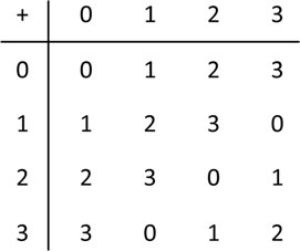
Figure 4.1:  Modulo-4 addition table with elements {0,1, 2, 3}.

To see why this is the case, we first assume that p is a prime number. Associativity and commutativity of modulo-p multiplication are obvious. The identity element is 1. ∈ is closed since there are no m, n ∈ G such that m · n = 0 modulo-p (otherwise p must divide m · n, but p and m · n are relatively prime since m, n < p and p is prime). Furthermore, every element of G has an inverse (see Problem 4.6.2). Therefore, G is a finite group under modulo-p multiplication.

The other direction of the proposition is easily seen by noting that if p is not a prime number, then there exist m,n ∈ G such that m · n = 0 modulo-p, i.e., the set is not closed under the modulo-p multiplication operation.

Modulo-5 multiplication table with elements {1, 2, 3, 4} is shown in Figure 4.2. Clearly, the set is closed under this binary operation, “1” is the identity element, and each element has an inverse (“1” is observed in each row exactly once).

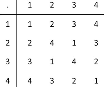
Figure 4.2:  Modulo-5 multiplication table with elements {1, 2, 3, 4}.

The number of elements in a group can be finite or infinite. For finite groups, we define the order of a group as the cardinality of the set G. The order of a group element g ∈ G is the smallest positive integer n such that

$\underset{n\hspace{0.17em}many}{\underbrace{g\cdot g\dots g}}=g^n=1,$

where “1” is the identity element of the group.

Example 4.1.3. Consider the group formed by {1, 2, 3, 4} under modulo-5 multiplication. The order of the group is 4. The orders of its elements are 1 (for 1), 2 (for 4), and 4 (for 2 and 3). Notice that the orders of different elements all divide 4 (the order of the group). This is not a coincidence as will become evident later.

Example 4.1.4. Consider the group {1, 2,…, 10} under modulo-11 multiplication. This group contains one element of order 1 (1), one element of order 2 (10), four elements of order 5 (3,4, 5 and 9) and four elements with order 10 (2, 6, 7 and 8). Again the possible orders (1, 2, 5 and 10) are integer factors of the order of the group.

Definition 4.1.2. Let H be a subset of G (where G forms a group under some binary operation “·”). If H satisfies the group properties under the same operation, then it is a subgroup of G.

Clearly, with this definition, H is closed under the binary operation “·”, it contains the identity element of the group, and for any element in H, the inverse is also contained in H.

Example 4.1.5. Consider G = {0,1, 2,…, 7} under modulo-8 addition. Clearly, the set H_i = {0, 2,4, 6} forms a subgroup under the same binary operation, so does the set H₂ = {0, 4}

Definition 4.1.3. Let H be a subgroup of G with the binary operation “·”. For a ∈ G, the set of elements a · H = {a · h : h ∈ H} is a left-coset of H, and H · a = {h · a : h ∈ H} is a right-coset.

For commutative groups, the left- and right-cosets are obviously identical, and they are simply referred to as a coset. It can be shown that no two elements in a coset are identical. To see this, consider an element a ∈ G and its left coset a · H. Enumerate the elements of H as H = {h₁, h₂,…, h_m}. Assume that there exist two distinct elements of H, h_i and h_j such that a · h_j = a · h_j. Applying the inverse of a to both sides, we obtain a⁻¹ · a · h_j = a⁻¹ · a · h_j, and from the associativity of the binary operation, we obtain h_j = h_j which is clearly a contradiction. The same argument holds for the case of right-cosets, and the claim is proved.

Similarly, it can also be proved that no two elements of two different cosets of H are identical (see Problem 4.6.4). In other words, distinct cosets of H are disjoint. Furthermore, every element of the group G is an element of one of the cosets of H (since for any b ∈ G, we can write b = (b · h⁻¹) · h for some h ∈ H). Combining these results, we can say that the order of a subgroup H divides the order of the group, and further its cosets form a partition of the group. Let us illustrate this result via a simple example.

Example 4.1.6. Consider G = {0,1, 2,…, 15} with modulo-16 addition, and its subgroup H = {0,4, 8,12}. There are four different cosets of H (since this is an abelian group, we do not make a distinction between the left- and right-cosets): {0, 4, 8,12}, {1, 5, 9,13}, {2, 6,10,14}, and {3, 7,11,15}. Clearly, the four cosets do not have any common elements and their union is G.

4.1.2      Rings

We now define a different algebraic structure with two binary operations.

Definition 4.1.4. A set of elements R with two operations “+” and “·” form a ring if

•  R is an abelian group under “+”,

•  “·” is associative,

•  “·” distributes over “+”, i.e., ∀a, b, c ∈ R, a · (b + c) = (a · b) + (a · c).

The ring is commutative if ∀a, b ∈ R, a · b = b · a.

It is clear that while a ring is an abelian group under the first operation “+”, it does not necessarily satisfy the properties of a group with respect to the second operation.

An important example of a ring is the set of polynomials. That is, the set of polynomials with real coefficients form a commutative ring with identity under the usual polynomial addition (“+” operation) and polynomial multiplication (“+” operation). The additive identity is 0, and the multiplicative identity is 1 (constants). A more important example for our purposes is the set of polynomials with binary coefficients that will be studied in more detail later in the chapter.

4.1.3      Fields

We are now in a position to define a field.

Definition 4.1.5. A set of elements F with two binary operations “+” (referred to as addition) and “·” (referred to as multiplication) form a field if

•  F is an abelian group under “+”. The additive identity of the field is denoted by “0”, and the additive inverse of a field element a is denoted by −a.

•  F {0} is an abelian group under “·”. The multiplicative identity is denoted by “1”, and the multiplicative inverse of a field element a ≠ 0 is denoted by a⁻¹.

•  The binary operation “·” distributes over the operation “+”.

We further define subtraction “−” and division “/” as

$a-b\triangleq a+\left(-b\right)$

and

$a/b\triangleq a\cdot \left(b^{-1}\right),\mathrm{if}\hspace{0.17em}b\ne 0.$

Also, sometimes we find it convenient to drop “·” when writing the multiplication of two elements, i.e., we use “ab” to represent “a · b”.

Common examples of fields include the set of real numbers under real addition and multiplication, the set of complex numbers under complex addition and complex multiplication, and the set of rational numbers under standard addition and multiplication. These fields clearly contain infinitely many elements (first two uncountably infinite, the latter countably infinite). For our purposes, however, finite fields are more important.

Example 4.1.7. If p is a prime number, the set of integers {0,1, 2,… , p − 1} form a field under modulo-p addition and modulo-p multiplication. It is easy to see this since modulo-p multiplication distributes over modulo-p addition, and we have already established in Section 4.1.1 that the set {0,1, 2,… ,p− 1} is an abelian group under modulo-p addition (regardless of what p is) with the identity element 0, and that the set {1, 2, 3,… ,p − 1} is an abelian group under modulo-p multiplication (if and only if p is a prime number).

Finite fields are also called Galois fields denoted by GF. For the field in Example 4.1.7, for instance, the notation is GF(p). If p = 2, we obtain the binary field denoted by GF(2) where the two operations are binary addition and binary multiplication as shown in Figure 4.3. Notice that binary addition and subtraction are the same since the additive inverses of both elements of GF(2) are themselves.

We can perform the usual arithmetic operations without any confusion or difficulty in a field. For instance, for any two elements of the field a, b, we can write −(a·b) = (−a) ·b = a· (−b) = −ab (see Problem 4.6.5). In a similar fashion, we can argue that cancellation of common multiplicative terms in an equation is possible (as long as the term being cancelled is non-zero). That is, if a · b = a · c and a ≠ 0, then b = c (easily seen by simply multiplying both sides of the equality by the multiplicative inverse of a which exists since a is a non-zero element). We can also argue that if two non-zero elements of the field are multiplied, the result cannot be zero (i.e., the additive identity). Furthermore, if a field element is multiplied by the additive identity, the result is the additive identity. In other words, if a ∈ F, then a · 0 = 0 since

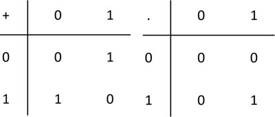
Figure 4.3:  Addition and multiplication tables in GF(2).

$\begin{array}{l}a·0=a·\left(b+\left(-b\right)\right)\\ \hspace{0.17em}\hspace{0.17em}\hspace{0.17em}\hspace{0.17em}\hspace{0.17em}\hspace{0.17em}\hspace{0.17em}\hspace{0.17em}\hspace{0.17em}\hspace{0.17em}\hspace{0.17em}=a·b+a·\left(-b\right)\\ \hspace{0.17em}\hspace{0.17em}\hspace{0.17em}\hspace{0.17em}\hspace{0.17em}\hspace{0.17em}\hspace{0.17em}\hspace{0.17em}\hspace{0.17em}\hspace{0.17em}\hspace{0.17em}=a·b+\left(-\left(a·b\right)\right)\\ \hspace{0.17em}\hspace{0.17em}\hspace{0.17em}\hspace{0.17em}\hspace{0.17em}\hspace{0.17em}\hspace{0.17em}\hspace{0.17em}\hspace{0.17em}\hspace{0.17em}\hspace{0.17em}=0.\end{array}$

We note that an immediate implication of an earlier example (Example 4.1.7) is that finite fields of a prime order (for any prime number) exist. However, it does not establish existence of fields of non-prime orders, and it does not address the question whether we can define a finite field of an arbitrary order or not. To partially address this question, we present an example of a field construction with four elements.

Example 4.1.8. Consider the elements F = {0,1, 2, 3} with the multiplication and addition table given in Figure 4.4.

One can easily verify that F along with the defined addition and multiplication operations form a field. For instance, it is clear that additive identity is 0, multiplicative identity is 1, the additive inverse of an element is itself, and the multiplicative inverses of the elements 1, 2, and 3 are 1, 3, and 2, respectively.

The example clarifies that there is a field of order 4 which is not a prime number. Further, it makes the point that to construct a field we may need to define the binary operations in a somewhat peculiar and nontrivial manner. For instance, using the very first approach that comes to mind, i.e., modulo-4 addition and multiplication operations, does not work.

Similar to the definition of a subgroup, we refer to a subset of field elements with the same two operations as a subfield if the subset satisfies the field properties. Clearly, the finite field in Example 4.1.8 (GF(4)) contains GF(2) as a subfield.

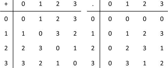
Figure 4.4:  Addition and multiplication tables for GF(4).

4.2      Galois Fields

We now describe details of finite fields, also referred to as Galois fields in honor of their inventor Évariste Galois, leading up to a full characterization of all possible finite fields and their construction in a subsequent section. Clearly, a finite field contains at least two elements, “0” (the additive identity) and “1” (the multiplicative identity). GF(2) described in the previous section is obviously the smallest field one can define.

Consider a finite field of order q denoted by GF(q) where q is not necessarily a prime number. It is easy to prove that when we add the multiplicative identity “1” repeatedly we will obtain the additive identity of the field at some point (since there are only a finite number of field elements). We define the characteristic of the field GF(q) as the smallest positive integer p such that

$\underset{p\hspace{0.17em}many}{\underbrace{1+1+\cdots +1}}={\displaystyle \sum _{i=1}^{p}1=0.}$

We note that the characteristic of a finite field is a prime number (otherwise ${\displaystyle {\sum }_{i=1}^{p}1}=\left({\displaystyle {\sum }_{i=1}^{m}1}\right)\left({\displaystyle {\sum }_{i=1}^{n}1}\right)=0$ for some non-negative integers m, n < p which leads to a contradiction).

A second observation is that GF(p) is a subfield of GF(q) with elements $\left\{0,1,1+1,1+1+1,\dots ,{\displaystyle {\sum }_{i=1}^{p-1}1}\right\}$. This can be confirmed by verifying that this subset along with the two binary operations of the original field satisfy the field properties. For instance, when two elements ${\displaystyle {\sum }_{i=1}^{m}1}$ and ${\displaystyle {\sum }_{i=1}^{n}1}$ are added, we obtain ${\displaystyle {\sum }_{i=1}^{k}1}$ with k = m + n modulo-p (utilizing ${\displaystyle {\sum }_{i=1}^{p}1}=0$), and when the two elements are multiplied, we obtain ${\displaystyle {\sum }_{i=1}^{l}1}$ with l = mn modulo-p (again noting that ${\displaystyle {\sum }_{i=1}^{p}1}=0$). Further, the additive inverse of ${\displaystyle {\sum }_{i=1}^{m}1}$ is ${\displaystyle {\sum }_{i=1}^{p-m}1}$ which is in the set. Similarly, there is a multiplicative inverse of any element of the form ${\displaystyle {\sum }_{i=1}^{m}1}$ (with m = 0) contained in the set. To see this, note that since p and m are relatively prime (1 < m < p – 1, and p is prime), there exist two positive integers r, s such that mr = ps + 1 (using Euclid’s algorithm for finding the greatest common divisor of two integers), i.e., mr = 1 modulo-p, therefore ${\displaystyle {\sum }_{i=1}^{m}1}$ has a multiplicative inverse in the set given by ${\displaystyle {\sum }_{i=1}^{r}1}$.

Let us denote the elements of GF(p) (which is a subfield of GF(q)) more compactly as {α₀,α₁,α₂,… ,a_p-1} (with the understanding that α₀ = 0 and α₁ = 1). Consider a non-zero element of GF(q), denoted by β₁. Then a_iß₁(i ∈ {0,1,… ,p – 1}) are p distinct elements of GF(q). If all the elements of GF(q) are accounted for in this list then q = p. If not, consider another element of GF(q), ß₂, not listed previously. Then a_iß₁ + ajß₂ (0 < i, j < p — 1) are p² distinct elements in GF(q). If there are no other elements, then q = p², otherwise consider an additional element ß₃, and form a_iß₁ + ajß₂ + a_kß₃ (0 < i, j, k < p – 1) to construct p³ distinct elements of GF(q). We continue this process until there are no other elements left uncovered in GF(q) to argue that the order of the field GF(q) must be a power of its characteristic, i.e., q = p^m for some integer m.

With the above argument we establish the following theorem.

Theorem 4.2.1. The order of a finite field GF(q) must be a power of a prime number.

We already know from an earlier example how to obtain GF(q) when q is prime: we simply can use the elements F = {0,1, 2,…, q — 1} with modulo-q addition and multiplication to define the field. However, the construction of GF(q) when q = p^m where p is a prime number and m > 1, is not that straightforward, and we need to approach the problem differently. It may be tempting to propose using modulo-q arithmetic, but this clearly does not work, as q — 1 is not prime, and we do not have a group structure for the non-zero elements under the multiplication operation.

Several other results regarding the properties of a finite field are considered in the following.

Theorem 4.2.2. The (q — 1)th power of a non-zero element of a finite field is 1, i.e., if a ∈ GF(q) and a ≠ 0, we have $a^{q-1}={\prod }_{i=1}^{q-1}a=1$.

Proof. See Problem 4.6.7.

□

Let us define the order of a non-zero element a ∈ GF(q) as the smallest integer n such that ${\prod }_{i=1}^{n}a=a^n=1$.

Theorem 4.2.3. The order of a non-zero element a ∈ GF(q) divides q — 1.

Proof. Consider a non-zero element a in the field with order n, i.e., the smallest integer for which aⁿ = 1 is n. Assume that n does not divide q — 1 and let the remainder obtained by dividing q — 1 by n be r, i.e., q — 1 = nk + r with 0 < r < i. We can write a^q-1 = a^nk+r, which implies that a^q-1 = (aⁿ)^ka^r from which we obtain a^r = 1 (since a^q-1 = 1 for any non-zero field element). This is a contradiction as 0 < r < n, hence r must be zero, i.e., n must divide q — 1.

□

A non-zero element a ∈GF(q) is called primitive if its order is q − 1. GF(q) contains at least one primitive element as an immediate corollary of the following theorem.

Theorem 4.2.4. The number of elements of order n in GF(q) (where n divides q − 1) is given by

$\phi \left(n\right)=n{\displaystyle \prod _{p|n}\left(1-\frac{1}{p}\right)}$

where p runs over all prime numbers (that divide n).

Proof. See [4] or any book on modern algebra.

□

φ(n) is called the Euler totient function and is the number of integers in {1, 2,… ,n− 1} that are relatively prime to n (including 1).

As a corollary to the theorem, we can easily conclude that there are exactly φ(q− 1) primitive elements in GF(q).

Example 4.2.1. Consider GF(16). There are φ(15) = 15(1 − 1/3)(1 − 1/5) = 8 primitive elements, $\phi \left(5\right)=5\left(1-\frac{1}{5}\right)=4$ elements of order 5 and φ(3) = 3(1 −1/3) = elements of order 2.

The rest of the chapter is devoted to the Galois fields with the characteristic p = 2, i.e., to the construction of extension fields of GF(2). The arguments and results directly extend to the extension fields of GF (p) where p is an arbitrary prime number; however, this generalization is omitted from our coverage. Before we proceed, we need to review some basic concepts about polynomials with binary coefficients.

4.3      Polynomials with Coefficients in GF(2)

We now discuss some basic properties of polynomials with coefficients from GF(2), which is of interest. A polynomial over GF(2) of degree-n is represented as

$f\left(X\right)=f_0+f_{1}X+f_2{X}^2+\cdots +f_n{X}^n$

with the understanding that “X” is an indeterminate and the coefficients (f_i’s) are taken from GF(2). We define the polynomial addition and multiplication operations as usual. Assume that f (X) and g(X) are two polynomials of degrees n and m with coefficients f₀, f₁,…, f_n and g₀, g₁,…, g_m, respectively. Without loss of generality assume that n ≥m. We define the polynomial addition as

$f\left(X\right)+g\left(X\right)=\left(f_0+g_0\right)+\left(f_1+g_1\right)X+\cdots +\left(f_m+g_m\right)X^m+f_{m+1}{X}^{m+1}+\cdots +f_n{X}^n$

and, the polynomial multiplication by

$f\left(X\right)\cdot g\left(X\right)=h_0+h_{1}X+h_2{X}^2+\cdots +h_{m+n}{X}^{m+n}$

where $h_i={\displaystyle {\sum }_{j=0}^i{f}_j{g}_{i-j}}$ (with the understanding that the g_i−j = 0 if i−j > m).

For instance, if f (X) = 1 + X + X³ and g(X) = X + X², we obtain

$f\left(X\right)+g\left(X\right)=1+X^2+X^3$

and

$f\left(X\right)\cdot g\left(X\right)=X+X^3+X^4+X^5,$

where we employed GF(2) addition and multiplication to determine the coefficients of the powers of the indeterminate X in the resulting polynomials.

With the two binary operations (polynomial addition and polynomial multiplication), the set of polynomials over GF(2) form a ring as can easily be verified.

Factorization of a polynomial in GF(2), or any other field, is an important notion. For instance, we can write

$X^3+1=\left(X+1\right)\left(X^2+X+1\right),$

i.e., X³ + 1 has two factors with coefficients again from GF(2). If a polynomial cannot be factorized into polynomials of smaller degrees over GF(2), it is said to be irreducible. For instance, it is not possible to factorize X² + X + 1 or X³ + X² + 1; hence, they are irreducible polynomials. We note, however, that it is still possible to factorize a polynomial in an extension field as will become apparent later in the chapter.

We digress here to point out that we are already familiar with similar statements in the context of a different field, namely, the complex number field. We can think of complex numbers as two-dimensional vectors (a, b) with a,b ∈ R (the first component being the real part and the second component being the imaginary part), or equivalently by a + jb where $j=\sqrt{-1}$. The addition of two complex numbers is defined as componentwise addition, i.e., (a, b) + (c, d) = (a + c, b + d), and multiplication of two complex numbers is defined through the operation (a, s) · (c, d) = (a · c − b · d, a · d+b · c). If we have a polynomial with coefficients from the real number field, it may be irreducible over the ground field, i.e. it may not have a real root; however, it is certainly reducible over the extension field of complex numbers. Considering the polynomial X² + 1 with real coefficients, the roots are complex conjugates of each other and are given by (0,1) and (0, −1). Since there are no real roots, the polynomial is irreducible over R. As another example, the polynomial (with coefficients in R) given by X³ − 1 has one real root, (1,0) and two complex roots, $\left(-1/2,\mp \sqrt{3}/2\right)$. Since it has a real root, it is reducible over R, and in fact we have X³ − 1 = (X − 1)(X² + X +1). Clearly the factors are irreducible over R. In general, any polynomial with real coefficients can be written as a unique product of degree-1 and irreducible degree-2 polynomials over R.

The following theorem is useful in the construction of GF(2^m).

Theorem 4.3.1. An irreducible polynomial with binary coefficients of degree-m divides $X^{2^m-1}+1$.

Proof. Refer to [1].

□

Definition 4.3.1. An irreducible polynomial over GF(2) of degree-m is called primitive if the smallest n such that the polynomial divides Xⁿ + 1 is n = 2^m − 1.

It is also a well-known result that primitive polynomials do exist. In fact, there are exactly φ>(2^m − 1)/m degree-m primitive polynomials over GF(2) where φ(#x00B7;) is the Euler totient function as defined earlier. Such polynomials are critical in the construction of Galois fields. Examples of primitive polynomials of degrees up to 10 are provided in Figure 4.5.

Figure 4.5:  Examples of primitive polynomials with coefficients from GF(2).

4.4      Construction of GF(2^m)

Let p(X) be a primitive polynomial of degree m with coefficients in GF(2). Assume that α is a root of that polynomial, i.e., p(α) = 0. Under this condition, the set of elements

$\left\{0,1,\alpha ,{\alpha }^2,\dots ,{\alpha }^{2^m-2}\right\}$

are all distinct. To see this, we simply note that α cannot be a root of a polynomial Xⁿ + 1 if n < 2^m − 1 (otherwise p(X) for which α is a root cannot be a primitive polynomial). In other words, choosing α as a root of a primitive polynomial of degree-m ensures that all the non-zero elements of GF(2^m) can be generated as its powers.

With this approach, multiplication of two field elements is trivial, we simply need to utilize ${\alpha }^{2^m-1}=1$. For the addition operation, we note that p(α) =0 and represent α^m as a polynomial in a with a degree less than m. In other words, we can write the elements as vectors of length m where each component denotes the corresponding coefficient (in GF(2)) of 1, α, α²,…, a^m−1, respectively. Notice that with this m-dimensional vector representation with binary coefficients, we can generate exactly 2^m elements (which are all the elements of the field GF(2^m)). Hence a suitable addition operation can also be defined for any two field elements by a simple componentwise addition.

Example 4.4.1. Consider GF(2³) generated by p(X) = 1 + X + X³. If α is a primitive element of the field, the entire set of elements can be written as F * = {0,1, α, α²,…,α⁶}. Taking a as a root of the primitive polynomial p(X) = 1 + X + X³, we have α³ = 1 + α. Using this relation, we can simply write the elements α⁴, α⁵ and α⁶ in terms of 1, α, and α² as:

$\begin{array}{l}{\alpha }^4=\alpha \cdot {\alpha }^3=\alpha \cdot \left(1+\alpha \right)=\alpha +{\alpha }^2,\\ {\alpha }^5=\alpha \cdot {\alpha }^4=\alpha \cdot \left(\alpha +{\alpha }^2\right)={\alpha }^2+{\alpha }^3=1+\alpha +{\alpha }^2,\\ {\alpha }^6=\alpha \cdot {\alpha }^5=\alpha +{\alpha }^2+{\alpha }^3=\alpha +{\alpha }^2+1+\alpha =1+{\alpha }^2.\end{array}$

For instance, for the addition of α⁵ and α³, we obtain α⁵ + α³ = 1 + α+α² + 1 + α =α² The complete addition and multiplication tables are shown in Figure 4.6.

Since we can construct GF(2³) using another primitive polynomial, it is clear that we can use a different primitive element, and obtain an entirely different addition table. Hence one may ask the question whether a finite field of a particular order is unique or not. This is answered by a fundamental result in finite field algebra which states that all such constructions are isomorphic, i.e., the Galois field of a particular order is unique up to a renaming of its elements [1].

To illustrate this point further, we present the following example.

Example 4.4.2. Consider GF(2³) generated by p(X) = 1 + X² + X³ which is also a primitive polynomial. Taking a primitive element of the field as a root of this polynomial, we can enumerate all the field elements as 0, 1, β, β²,

$\begin{array}{l}{\beta }^3=1+{\beta }^2,\\ {\beta }^4=\beta \cdot {\beta }^3=\beta \cdot \left(1+{\beta }^2\right)=\beta +{\beta }^3=1+\beta +{\beta }^2,\\ {\beta }^5=\beta \cdot {\beta }^4=\beta \cdot \left(1+\beta +{\beta }^2\right)=\beta +{\beta }^2+{\beta }^3=1+\beta ,\\ {\beta }^6=\beta \cdot {\beta }^5=\beta \left(1+\beta \right)=\beta +{\beta }^2.\end{array}$

Figure 4.7 shows the addition and multiplication tables obtained with this construction. It may not be obvious, but it is easy to check that by renaming the elements of GF (2³) as

$\begin{array}{c}\hspace{0.17em}\hspace{0.17em}\hspace{0.17em}0\leftrightarrow 0\\ \hspace{0.17em}\hspace{0.17em}\hspace{0.17em}1\leftrightarrow 1\\ \hspace{0.17em}\hspace{0.17em}\hspace{0.17em}\hspace{0.17em}\hspace{0.17em}\hspace{0.17em}\beta \leftrightarrow {\alpha }^6\\ {\beta }^2\leftrightarrow {\alpha }^5\\ {\beta }^3\leftrightarrow {\alpha }^4\\ {\beta }^4\leftrightarrow {\alpha }^3\\ {\beta }^5\leftrightarrow {\alpha }^2\\ {\beta }^6\leftrightarrow \alpha \end{array}$

we obtain the binary operation table given in Figure 4.6. In other words, the constructions for this example and for Example 4.4.1 are equivalent up to a renaming of the elements.

Now that we have constructed the finite field GF(2^m), it should be clear that we can perform usual arithmetic operations using its elements and the corresponding multiplication and addition rules. For instance, the following example illustrates the process of solving a set of linear equations.

Example 4.4.3. Consider the finite field GF(2⁴). Let α be a primitive element, and a root of 1 + X + X⁴. We are interested in solving for the unknowns X and Y which satisfy

$\begin{array}{c}{\alpha }^{3}X+{\alpha }^{2}Y={\alpha }^7\\ {\alpha }^{7}X+{\alpha }^{12}Y={\alpha }^3.\end{array}$

We first note that the elements α⁴, α⁵,…, α¹⁴ of GF(2⁴) can be written as

$\begin{array}{c}{\alpha }^4=\alpha +1,\\ {\alpha }^5={\alpha }^2+\alpha ,\\ {\alpha }^6={\alpha }^3+{\alpha }^2,\\ {\alpha }^7={\alpha }^3+\alpha +1,\\ {\alpha }^8={\alpha }^2+1,\\ {\alpha }^9={\alpha }^3+\alpha ,\\ {\alpha }^{10}={\alpha }^2+\alpha +1,\\ {\alpha }^{11}={\alpha }^3+{\alpha }^2+\alpha ,\\ {\alpha }^{12}={\alpha }^3+{\alpha }^2+\alpha +1,\\ {\alpha }^{13}={\alpha }^3+{\alpha }^2+1,\\ {\alpha }^{14}={\alpha }^3+1.\end{array}$

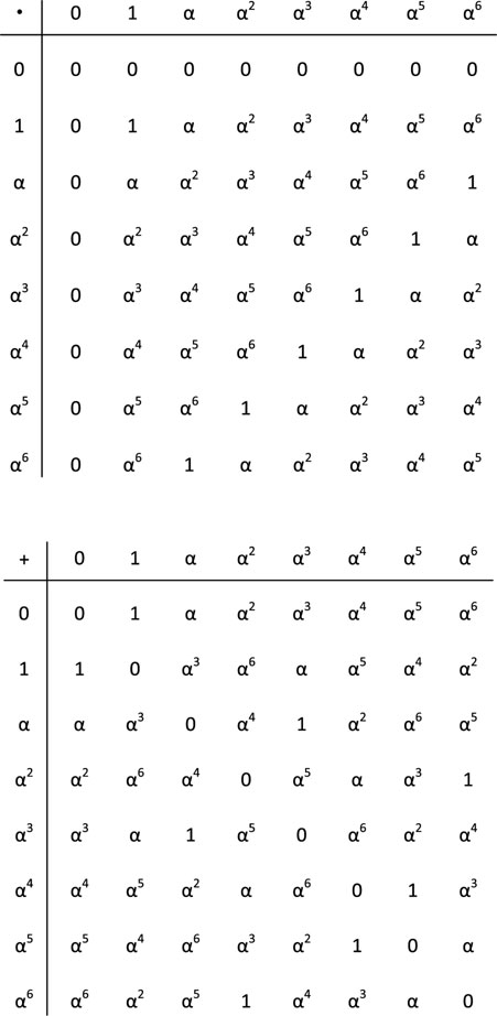
Figure 4.6:  Multiplication (top) and addition (bottom) tables for GF(2³) generated by the primitive polynomial 1 + X + X³.

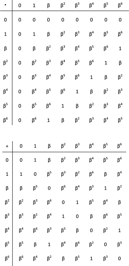
Figure 4.7:  Multiplication (top) and addition (bottom) tables for GF(2³) generated by the primitive polynomial 1 + X² + X³.

Multiplying the first equation by α⁴ and adding the two equations, we obtain

$\left({\alpha }^7+{\alpha }^7\right)X+\left({\alpha }^6+{\alpha }^{12}\right)Y={\alpha }^{11}+{\alpha }^3.$

Since α⁷ + α⁷ = 0, α⁶ + α¹² = α³ + α² + α³ + α² + α + 1 = α + 1 = α⁴, and α¹¹ + α³ = α³ + α² + α + α³ = α² + α = α⁵, we obtain α⁴Y = α⁵, and Y = α. Substituting this into the first original equation gives α³X + α²α = α⁷, which results in X = α.

Although linear equations are solved with ease, the same may not be true for non-linear equations. In general, we would need to substitute all the elements of the Galois field into the set of equations being solved to identify the solutions. For instance, finding the roots of a polynomial in an extension field is not trivial, nor computing logarithms (i.e., performing inverse of exponentiation).

4.4.1      Conjugate Elements

We can define conjugates of an element of finite field akin to the conjugate of a number in the complex number field. We start with a basic result.

Theorem 4.4.1. If b ∈ GF(2^m) is a root of a polynomial p(X) over GF(2), then $b^{2^k}$ is also a root of the same polynomial for any non-negative integer k.

Proof. Let p(X) = p₀ + p₁X + … + p_nXⁿ, we can easily write

$\begin{array}{l}{\left(p\left(X\right)\right)}^2={\left(p_0+p_{1}X+\cdots +p_n{X}^n\right)}^2\\ \hspace{0.17em}\hspace{0.17em}\hspace{0.17em}\hspace{0.17em}\hspace{0.17em}\hspace{0.17em}\hspace{0.17em}\hspace{0.17em}\hspace{0.17em}\hspace{0.17em}\hspace{0.17em}\hspace{0.17em}\hspace{0.17em}\hspace{0.17em}\hspace{0.17em}\hspace{0.17em}\hspace{0.17em}\hspace{0.17em}\hspace{0.17em}\hspace{0.17em}=p_0^2+p_1^2{X}^2+\cdots +p_n^2{X}^{2n}\\ \hspace{0.17em}\hspace{0.17em}\hspace{0.17em}\hspace{0.17em}\hspace{0.17em}\hspace{0.17em}\hspace{0.17em}\hspace{0.17em}\hspace{0.17em}\hspace{0.17em}\hspace{0.17em}\hspace{0.17em}\hspace{0.17em}\hspace{0.17em}\hspace{0.17em}\hspace{0.17em}\hspace{0.17em}\hspace{0.17em}\hspace{0.17em}\hspace{0.17em}=p_0+p_1{X}^2+\cdots +p_n{X}^{2n}\\ \hspace{0.17em}\hspace{0.17em}\hspace{0.17em}\hspace{0.17em}\hspace{0.17em}\hspace{0.17em}\hspace{0.17em}\hspace{0.17em}\hspace{0.17em}\hspace{0.17em}\hspace{0.17em}\hspace{0.17em}\hspace{0.17em}\hspace{0.17em}\hspace{0.17em}\hspace{0.17em}\hspace{0.17em}\hspace{0.17em}\hspace{0.17em}\hspace{0.17em}=p\left(X^2\right).\end{array}$

The second and third lines follow since the coefficients and the operations are in GF(2). Continuing in this manner, we find that ${\left(p\left(X\right)\right)}^{2^k}=p\left(X^{2^k}\right)$. Hence, if p(b) = 0, we also have $p\left(b^{2^k}\right)=0$, and the proof is complete.

As a side note, consider the complex number field. If a polynomial with real coefficients has a particular complex number as one of its roots, then the complex conjugate of the number is also a root - similar to the result of this theorem (which applies in the context of finite fields).

Definition 4.4.1. The elements of the field of the form $b^{2^k}$ are defined as the conjugates of b. Obviously, we have a finite number of conjugates for any element of the Galois field as there are only finitely many distinct elements. The set of all conjugates of b is referred to as the conjugacy class of the element b.

Definition 4.4.2. The smallest degree polynomial ϕ(X) over GF(2) such that ϕ(b) = 0 (b ∈ GF(2^m)) is called the minimal polynomial of b. Note that the minimal polynomial is unique. To see this, assume that there are two distinct degree-n minimal polynomials ϕ₁(X), φ₂(Χ) for a particular element. Then their sum (which is a polynomial of a smaller degree as Xⁿ terms cancel out) also has the same element as a root, which is a contradiction.

Theorem 4.4.2. The minimal polynomial of any element of GF (2^m) is irreducible over GF(2).

Proof. Assume that it is not irreducible, and write ϕ(Χ) = ϕ₁(Χ)ϕ₂(Χ). Then, ϕ₁(b)ϕ₂(b) = 0, hence either ϕ₁ = 0 or ϕ₂(b) = 0 which is a contradiction.

Theorem 4.4.3. If p(b) = 0 for a binary polynomial p(X) and b ∈ GF(2^m), then the minimal polynomial of b divides p(X).

Proof. See Problem 4.6.9.

□

As a corollary, we can say that if p(X) is an irreducible polynomial with binary coefficients and p(b) = 0 for b ∈ GF(2^m), then p(X) is the minimal polynomial of b.

Theorem 4.4.4. The minimal polynomials of the elements of GF(2^m) divide $X^{2^m}+X$ (also including the minimal polynomial for the additive identity “0”).

Theorem 4.4.5. If the distinct conjugates of b ∈ GF (2^m) are b₂,…,b_n(and let b₁ = b), then its minimal polynomial is given by

$\varphi \left(X\right)={\displaystyle \prod _{i=1}^n\left(X+b_i\right).}$

We further note that n ≤ m, and hence the degree of the minimal polynomial ϕ(X) is at most m.

Proof. See [1].

□

Example 4.4.4. Consider GF(2⁴). Let b = α⁵ where α is a primitive element of the field (and a root of the primitive polynomial 1 + X + X⁴). Then the conjugate of b is b₂ = b² = α¹⁰ (note b⁴ = α²⁰ = α⁵ = b). Therefore, the minimal polynomial for b = α⁵ is

$\varphi \left(X\right)=\left(X+{\alpha }^5\right)\left(X+{\alpha }^{10}\right)=1+X+X^2.$

Similarly, for the element α⁶ ∈ GF(2⁴), the conjugates are α¹², α⁹ and α³, and the corresponding minimal polynomial is

$\begin{array}{l}\varphi \left(X\right)=\left(X+{\alpha }^6\right)\left(X+{\alpha }^{12}\right)\left(X+{\alpha }^9\right)\left(X+{\alpha }^3\right)\\ \hspace{0.17em}\hspace{0.17em}\hspace{0.17em}\hspace{0.17em}\hspace{0.17em}\hspace{0.17em}\hspace{0.17em}\hspace{0.17em}\hspace{0.17em}\hspace{0.17em}\hspace{0.17em}\hspace{0.17em}\hspace{0.17em}=1+X+X^2+X^3+X^4.\end{array}$

The details of this computation are left as an exercise (see Problem 4.6.11).

□

4.4.2      Factorization of the Polynomial Xⁿ + 1

An important issue in channel coding, particularly in the design of cyclic codes, is the factorization of the polynomial of the type Xⁿ + 1 over GF(2). For instance, the factors of this polynomial can be used as generator polynomials for a cyclic code of length n bits. For the special case where n = 2^m − 1, the process of factoring Xⁿ + 1 relies on the ideas developed earlier in the section with the observation that we already have a tool to generate minimal polynomials of all the elements of GF (2^m), and the roots of these polynomials define the corresponding conjugacy classes. A strongly related result further states that the factors of $X^{2^m}+X$ are all irreducible polynomials of degrees that divide m (see [1]), and all the elements of GF (2^m) are the roots of the binary polynomial $X^{2^m}+X$.

The factors of $X^{2^m-1}+1$ are simply the minimal polynomials of the non-zero elements of GF(2^m). Let us illustrate this computation by a simple example.

Example 4.4.5. Consider GF(2³) generated by p(X) = 1 + X + X³, and the minimal polynomials of its elements to factorize the binary polynomial X⁷ + 1. The minimal polynomial for 1 is X + 1, for the elements α, α², α⁴, the minimal polynomial is (X + α)(X + α²)(X + α⁴) = 1 + X + X³ (assuming that α is a root of the primitive polynomial p(X) = 1+X+X³), and for α³, α⁶, α⁵, the corresponding minimal polynomial is (X + α³)(X + α⁶)(X + α⁵) = 1 + X² + X³. Hence, we can factorize X⁷ + 1 as

$X^7+1=\left(X+1\right)\left(X^3+X+1\right)\left(X^3+X^2+1\right).\hspace{0.17em}\square$

We give a similar example in the following.

Example 4.4.6. To factorize the binary polynomial X¹⁵ + 1, let us consider the GF(2⁴) generated by the primitive polynomial 1 + X + X⁴. Let a be a root of this polynomial. Then the conjugacy classes of the non-zero elements of the field are

$\begin{array}{c}\left\{1\right\},\\ \left\{\alpha ,{\alpha }^2,{\alpha }^4,{\alpha }^8\right\},\\ \left\{{\alpha }^3,{\alpha }^6,{\alpha }^{12},{\alpha }^9\right\},\\ \left\{{\alpha }^5,{\alpha }^{10}\right\},\\ \left\{{\alpha }^7,{\alpha }^{14},{\alpha }^{13},{\alpha }^{11}\right\},\end{array}$

and the corresponding minimal polynomials (after some algebra) are

$\begin{array}{c}X+1\\ X^4+X+1\\ X^4+X^3+X^2+X+1,\\ X^2+X+1,\end{array}$

$X^4+X^3+1.$

Therefore, we can factorize X¹⁵ + 1 as

$X^{15}+1=\left(X+1\right)\left(X^4+X+1\right)\left(X^4+X^3+1\right)\left(X^4+X+1\right)\left(X^4+X^3+X^2+X+1\right).\hspace{0.17em}\square$

For an arbitrary positive integer n, the factorization of Xⁿ + 1 follows a similar procedure. The main difference is that there is not a field of size n + 1 in general, and we cannot work with a primitive element of such a field to generate conjugacy classes. Therefore, we identify an extension field GF(2^m) such that n is a factor of 2^m − 1. Therefore, there exists an element β ∈ GF(2^m) with order n, and we can work with the minimal polynomials of the powers of β. The product of the distinct resulting minimal polynomials are factors of Xⁿ +1. Let us give two simple examples to conclude the section.

Example 4.4.7. To factorize X⁵ + 1, we consider the extension field GF(2⁴) as 5 divides 2⁴ − 1. Let b be an element of GF(2⁴) with order 5, i.e., b⁵ = 1. Clearly, b = α³ where α is a primitive element of GF(2⁴). There are two conjugacy classes with respect to b: {1} and {b, b², b⁴, b³}. The corresponding minimal polynomials are X + 1 and X⁴ + X³ + X² + X + 1, hence

$X^5+1=\left(X+1\right)\left(X^4+X^3+X^2+X+1\right).\hspace{0.17em}\square$

Example 4.4.8. Let us factorize X¹³ + 1. Consider an element b in an extension field of GF(2) with order 13 (such elements are present in GF(2¹²) as 13 divides 2¹² − 1 = 4095). Then the conjugacy classes are

$\left\{1\right\},$

and

$\left\{b,b^2,b^4,b^8,b^3,b^6,b^{12},b^{11},b^9,b^5,b^{10},b^7\right\}.$

Therefore, there are two irreducible factors of X¹³ + 1. In fact, we can write

$X^{13}+1=\left(X+1\right)\left(X^{12}+X^{11}+X^{10}+X^9+X^8+X^7+X^6+X^5+X^4+X^3+X^2+X+1\right).\hspace{0.17em}\square$

4.5      Some Notes on Applications of Finite Fields

We close this chapter by highlighting a couple of applications of Galois fields, in particular, for channel coding and cryptography. Consider transmission of digital information, 0's and 1's, over a noisy channel. In order to protect the information bits against channel errors, it is a common practice to map the message sequence to a coded sequence of bits, and transmit the resulting codeword. At the receiver side, occasional channel errors are identified (and/or corrected), by utilizing the controlled redundancy in the codewords. This process is referred to as channel coding and is an integral part of any modern digital communication system. The second application area, cryptography, refers to the process of communication with an intended receiver (loosely speaking) while making sure that a third party (eavesdropper) cannot decode the message bits even if it has access to the entire transmitted sequence.

Cyclic codes represent a fairly general and widely employed channel coding method. Let us consider a message sequence of length k-bits as a degree k − 1 polynomial over GF(2), i.e., represent the message bits m_i, i ∈ {0,1,…,k − 1} with the polynomial m(X) = m₀ + m₁X + m₂X²+… + m_k−1X^k−1. Define a factor of the polynomial Xⁿ + 1 as the generator polynomial of a cyclic code denoted by g(X) (of degree n− k). We can then obtain a specific channel code by considering the codeword polynomials as the product of the message polynomial with the generator polynomial, i.e.,

$c\left(X\right)=m\left(X\right)\cdot g\left(X\right).$

The coefficients of c(X) determine the components of the n-bit long codeword sequence. It should now be clear that the theory of finite fields is needed for a complete study of such coding schemes. For instance, by using the ideas in the previous section, one can determine possible dimensions of all cyclic codes, i.e., figure out for what values of n and k, cyclic codes do or do not exist.

As an example, consider the factorization of the binary polynomial X²³ + 1 using the techniques described in this chapter. There are three irreducible factors: X + 1 and two degree-11 polynomials. Therefore, we can define a cyclic code of dimensions n = 23 and k = 12 using either one of the two degree-11 factors as its generator polynomial. The so-obtained codes are named “Golay codes” and have a beautiful algebraic structure and desirable properties. They have been employed in practical communication systems including those utilized in deep-space missions of the National Aeronautics and Space Administration (NASA).

Reed-Solomon (RS) codes can also be cited as specific examples of cyclic codes. These codes find widespread applications in existing communication systems, for instance, in magnetic recording systems (hard drives), compact discs (CD), digital versatile discs (DVD), blue-ray disks, etc. When there are scratches on a DVD, the RS code ensures that the digital data can be recovered and accessed reliably. To describe the connection to the theory of Galois fields, consider a specific case with 255 bytes (2040 bits) as codewords correcting t many byte errors. This RS code may be obtained by a generator polynomial with coefficients in GF(2⁸) with the roots α, α²,…,α^2t where α is a primitive element of GF(2⁸) and t is an integer selected based on the desired error correction capability of the code (which comes at the cost of a reduced code rate). We refer the reader to textbooks on channel coding for the details of different algebraic code constructions, analysis and decoding algorithms, e.g. [3, 4].

As a particular instance of a crypto-system that utilizes finite field algebra, let us consider public key cryptography, where all the users advertise their own keys and encryption takes place by obtaining a common key between user pairs with the publicly available information. For instance, the users can pick an element of a high order finite field α^m (where α is a primitive element of the field), and make m publicly available (while α^m is kept secret). A common key between two users can then be easily generated by performing a simple exponentiation. For instance, if users A and B advertise m_A and m_B, they both can compute ${\left({\alpha }^{m_B}\right)}^{m_A}={\left({\alpha }^{m_A}\right)}^{m_B}={\alpha }^{m_A{m}_B}$ as their common key. However, without the knowledge of the primitive element of the field, it is extremely difficult for an eavesdropper to compute the key due to the inefficiency of the algorithms for calculating logarithms in a finite field.

4.6      Exercises

Exercise 4.6.1. Prove that the inverse of a group element is unique.

Exercise 4.6.2. Consider G = {1, 2, 3,…,p − 1} with modulo-p multiplication where p is a prime number. Prove that every element has an inverse, i.e., for any a ∈ G, there exists b ∈ G such that a · b =1 modulo-p.

Exercise 4.6.3. Consider the group {1, 2,…, 6} with modulo-7 multiplication. Show the multiplication table. Specify the inverse of each element. Also determine the orders of all the elements.

Exercise 4.6.4. Prove that no two elements of two different cosets of a subgroup H (of a group G) can be identical.

Exercise 4.6.5. For any two elements of a finite field a,b ∈ F, show that −(a· b) = (−a) · b = a · (−b).

Exercise 4.6.6. If a, b, c are field elements, show that if a · b = a · c and a ≠ 0, then b = c.

Exercise 4.6.7. Assume that a is a non-zero element of a finite field of order q. Prove that a^q−1 = 1.

Exercise 4.6.8. Consider GF(2³) and assume that α is a root of the primitive polynomial 1 + X + X³. Solve for X, Y, Z if

$\begin{array}{c}\alpha X+Y+{\alpha }^{3}Z={\alpha }^5\\ {\alpha }^{3}Y+\alpha Y=\alpha \\ {\alpha }^{5}X+{\alpha }^{2}Z={\alpha }^3.\end{array}$

Exercise 4.6.9. Let p(X) be a polynomial over GF(2), and b be an element of GF(2^m). Prove that if f (b) = 0, then the minimal polynomial of b, ϕ(X), divides p(X).

Exercise 4.6.10. Prove that degree of the minimal polynomial of an element of GF(2^m) is at most m.

Exercise 4.6.11. Show the details of the minimal polynomial computation in Example 4.4.4.

Exercise 4.6.12. Find the degrees of the minimal polynomials of the Galois field elements of order 15 and 1023 (with respect to GF(2)). Specify examples of Galois fields that contain these elements.

Exercise 4.6.13. How many binary irreducible polynomials exist in the factorization of X²⁵ + 1? Also find the degrees of the different factors.

References

[1]  R. J. McEliece, Finite Fields for Computer Scientists and Engineers. Boston: Kluwer Academic Publishers, 1987.

[2]  R. Lidl and H. Niederreiter, Introduction to Finite Fields and Their Applications. Cambridge: Cambridge University Press, 1986.

[3]  S. Lin and D. J. Costello, Jr.., Error Control Coding: Fundamentals and Applications, 2nd ed. Upper Saddle River, NJ: Prentice Hall, 2004.

[4]  S. B. Wicker, Error Control Systems for Digital Communications and Storage. Upper Saddle River, NJ: Prentice Hall, 1995.

[5]  H. C. A. van Tilborg, An Introduction to Cryptology. Boston: Kluwer Academic Publishers, 1988.